J. R. Barbosa, Jr.
Departamento de Engenharia Mecânica Universidade Federal de Santa Catarina 88040-900 Florianópolis, SC. Brazil [email protected]
Two-Phase Non-Equilibrium Models:
the Challenge of Improving Phase
Change Heat Transfer Prediction
This lecture addresses some recent developments in modelling of macroscopic thermodynamic and hydrodynamic non-equilibrium phenomena in convective phase change (boiling and condensation) of pure fluids and mixtures. Proper accounting of such phenomena may hold the key to explain and predict deviations from the classical (equilibrium) phase change convective heat transfer behaviour reported in the literature and yet not fully understood.
In the first part of the paper, a detailed qualitative description of the classical heat transfer coefficient behaviour is presented together with two examples of departure from macroscopic equilibrium largely supported by experimental evidence. The second part of the paper reviews successful attempts to model the non-equilibrium phase change phenomena taking place in the two situations.
The first example is a thermodynamic non-equilibrium slug flow model (one in which saturated Taylor bubbles become separated by slugs of subcooled liquid) that predicts the peaks in heat transfer coefficient at near-zero thermodynamic quality observed in forced convective boiling of some pure liquids. The occurrence of such peaks is typical of low latent heat, low thermal conductivity systems and of systems in which the vapour volume formation rate for a given heat flux is large.
The second example is a comprehensive annular flow calculation methodology that predicts the decrease in the heat transfer coefficient with increasing quality observed in convective boiling of binary and multicomponent mixtures. In this case, as will be seen, coupled mass transfer resistance and hydrodynamic non-equilibrium effects generate concentration gradients between the liquid film and entrained droplets that are responsible for the heat transfer deterioration. In addition,
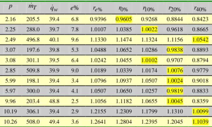
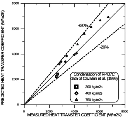
it will be shown that for condensation of mixtures the methodology predicts a heat transfer intensification which has been subsequently confirmed by independent experimental results.
Keywords: Two-phase flow, phase change, non-equilibrium modelling, slug flow, annular flow
Introduction
This paper is dedicated to the study of forced convective boiling of pure fluids and mixtures. Non-equilibrium models are reviewed in an attempt to explain situations in which departure from the classical (i.e., textbook) heat transfer coefficient behaviour takes place. Experimental conditions under which such deviations were observed are typical of most industrial phase change equipment.
A substantial portion of industrial heat exchange processes involve phase change at low to moderate heat fluxes (Hewitt et al., 1994), thus making phenomenological flow pattern based models for intermittent (e.g., slug) and wall film (e.g., churn and annular-dispersed) flows an attractive tool for improving existing design methods traditionally built upon equilibrium correlations (Webb and
Gupte, 1992; Collier and Thome, 1994).1
The major challenges in flow regime based modelling are the sound interpretation of observed non-equilibrium phenomena and their adequate representation aiming at the improvement of heat transfer predictions. Two types of non-equilibrium effects will be dealt with in this lecture, namely, thermodynamic non-equilibrium, that resulting from local departures from saturation (subcooling or superheating) with implications on the distribution of phases and of phase velocities within the heated channel; and hydrodynamic non-equilibrium, that resulting from phase and phase velocities distributions within the channel (e.g., slippage and droplet
Presented at ENCIT2004 – 10th Brazilian Congress of Thermal Sciences and Engineering, Nov. 29 -- Dec. 03, 2004, Rio de Janeiro, RJ, Brazil.
Technical Editor: Atila P. Silva Freire.
entrainment) with implications on the local thermodynamic balance within and between the phases.
The non-equilibrium effects treated in the present work extend from low to high qualities and are concerned with phase change of pure fluids as well as mixtures. There is, therefore, a great potential for incorporating such formulations in design methods. For instance, as pointed out by Wadekar and Kenning (1990), a considerable number of industrial reboilers operates in conditions typical of intermittent flows. Recent experimental (Urso et al., 2002) as well as modelling (Sun et al., 2004) efforts are being made to better understanding the particular features of such flows in the context of phase change equipment.
In what follows, Section 2 reviews important concepts related to the definition of thermodynamic and hydrodynamic equilibrium in forced convective flows with phase change. In Section 3, two examples extensively reported in the literature of departure from the equilibrium representation of the heat transfer coefficient behaviour in convective boiling are presented. The first example is the occurrence of heat transfer peaks in the near-zero quality region and the second example is the deterioration of heat transfer coefficient for binary and multicomponent mixtures at high qualities. Phenomenological models based on thermal and hydrodynamic non-equilibrium effects put forward by the present author and collaborators are reviewed in Sections 4 and 5. Finally, conclusions and recommendations for future work are presented in Section 6.
Some Equilibrium Phase Change Definitions
of the heat transfer coefficient behaviour will be presented at the end of this section.
Heat Transfer Coefficient
The local, time-averaged heat transfer coefficient is defined as,
b w
w
T T
q
− =
α , (1)
where q is the wall heat flux, w T is the local, time-averaged wall w
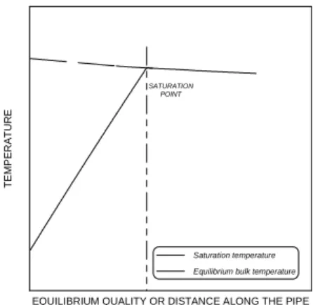
temperature and Tb is the local, time-averaged bulk temperature. In
the region downstream of the saturation point, Tb =Tsat
( )
p , wherepis the local pressure. Figure 1 illustrates the profiles of T and b
sat
T for a pure fluid at constant wall heat flux.
EQUILIBRIUM QUALITY OR DISTANCE ALONG THE PIPE
TE
M
P
E
R
A
T
U
R
E
Saturation temperature
Equilibrium bulk temperature SATURATION
POINT
Figure 1. Bulk and saturation temperature profiles as a function of distance along the pipe. Constant wall heat flux.
In boiling of liquid mixtures,Tb is the local bubble-point
temperature, Tbub. Alternatively, in condensation of vapour
mixtures, Tb is the local dew-point temperature, Tdew.
Quality
The equilibrium quality is defined as,
sat L sat G
sat L eq
h h
h h x
, ,
,
− −
≡ , (2)
where his the local specific enthalpy of the fluid (single phase or two-phase) and hL,satand hG,sat are the saturated liquid and vapour
enthalpies, respectively. Thus, in the two-phase saturated region,
sat G sat
L h h
h, ≤ ≤ , and 0≤xeq≤1. In the subcooled region,
sat L
h
h< , and xeq<0 and in the superheated region h>hG,sat
and xeq>0.
The vapour dynamic mass fraction (or the real or hydrodynamic quality) is defined as the ratio of the mass flow rate of vapour and the total mass flow rate,
L G
G G
M M
M x
+
≡ . (3)
As opposed to the equilibrium quality, the real quality varies only between 0 and 1, and is independent of the local thermodynamic state (saturated, subcooled or superheated). The
behaviour of xeqand xG as a function of enthalpy is illustrated in
Figure 2.
‘liquid still’
x
h
sat L
h, hG,sat 1
0
eq
x
G
x
‘vapour already’
Subcooling Saturation Superheating
Figure 2. An illustration of the difference between the equilibrium and the real quality.
In real flows in vaporization equipment, due to radial gradients of superheat (higher temperatures near the wall), bubble generation takes place adjacent to the wall whilst the bulk is still subcooled. This explains the existence of the region labelled as ‘vapour already’ in Figure 2. Analogously, the ‘liquid still’ region in Figure 2 accounts for the coexistence of superheated vapour and liquid droplets in the high quality region. In great part of the saturated region, however, there is a superposition of equilibrium and real qualities, enabling the convenient determination of vapour flow rates from energy balances. A more detailed exploration of the definitions of quality was provided by Baehr and Stephan (1998).
Regimes in Convective Boiling and the Classical Heat Transfer Coefficient Behaviour
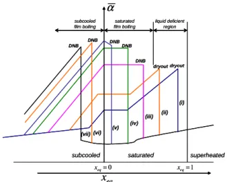
The classical (i.e., textbook) interpretation of the flow and heat transfer problem in convective boiling is presented through an analysis of Figures 3 and 4, adapted from Collier and Thome (1994). In Figure 3, the heat transfer regimes in convective boiling are represented qualitatively as a function of enthalpy (hence equilibrium quality) and wall heat flux. Figure 4 presents the qualitative behaviour of the heat transfer coefficient as a function of equilibrium quality and of heat flux. The total mass flow rate and the pipe geometry (length and diameter) are assumed constant and, for simplicity, the pressure drop is assumed negligible.
Single phase Convection (liquid)
Subcooled nucleate boiling
Saturated nucleate boiling Saturated
film
boiling Mist flow
evaporation
Single phase convection
(vapour)
Domain of liquid film evaporation w
q
h
sat L
h, hG,sat
(xeq=0) (xeq=1) Region of Departure from Nucleate Boiling (DNB)
Region of liquid film dryout
Transition between heat transfer mechanisms (nucleate boiling – evaporation)
Typical physical burnout locus Subcooled
film boiling
(i) (ii) (iii) (iv) (v) (vi) (vii)
(i)
(ii) (iii) (iv) (v) (vi) (vii)
dryout dryout DNB DNB DNB DNB DNB
subcooled saturated superheated
α
eq
x
0
=
eq
x xeq=1
subcooled film boiling
saturated film boiling
liquid deficient region
(i) (ii) (iii) (iv) (v) (vi) (vii)
dryout dryout DNB DNB DNB DNB DNB
subcooled saturated superheated
α
eq
x
0
=
eq
x xeq=1
subcooled film boiling
saturated film boiling
liquid deficient region
Figure 4. Qualitative heat transfer coefficient behaviour as a function of equilibrium quality and heat flux (Collier and Thome, 1994).
In Figures 3 and 4, lines (i) to (vii) represent increasing heat flux conditions. Curve (i) relates to a low heat flux condition, and together with curve (ii), envelope the (design) operating conditions of two-phase heat transfer equipment (e.g., evaporators, reboilers etc.). Flow patterns within this range of heat fluxes are typically those observed in adiabatic gas-liquid flows (i.e., bubble, slug, churn, annular and mist flows). Liquid depletion in the near wall region takes place at relatively high qualities and is associated with the phenomenon of liquid film ‘dryout’ (rather than the departure from nucleate boiling – DNB – typical of high heat fluxes – for more details see Collier and Thome, 1994).
All of the non-equilibrium effects reported in this paper occur within the low heat flux range of the boiling region illustrated in Figures 3 and 4 (curves i and ii). In this region, starting with heat transfer to saturated liquid near the entrance of the channel, subcooled boiling is initiated giving rise to an increasing heat transfer coefficient (defined in this region as the rate of the wall heat flux to the difference between the wall temperature and the bulk temperature). After equilibrium saturation has been attained, the heat transfer coefficient (now defined as the ratio of the wall heat flux to the difference between the wall temperature and the saturation temperature) remains approximately constant and independent of quality (reflecting the dominance of nucleate boiling effects). Further downstream, as quality increases, there is a transition to a heat transfer mode dominated by forced convection and the heat transfer coefficient increases with increasing quality up to the point of critical heat flux (CHF), characterized by the ‘dryout’ of the liquid film.
Departure from the Classical Behaviour
As pointed out by Hewitt (2000), the representation of the heat transfer coefficient behaviour delineated in Section 2 has been the basis of design calculations for forced convective boiling for many years, with correlations being developed to represent the various regions of Figures 3 and 4. In this section, the non-equilibrium phenomena responsible for substantial departures from this classical representation will be identified. Physical interpretations of these phenomena will be provided together with phenomenological models for their prediction.
Heat Transfer Peaks at Near-Zero Qualities
The first case of departure from the classical behaviour of convective boiling heat transfer is the occurrence of heat transfer coefficient peaks in the region of near-zero equilibrium quality. The peaks were observed in boiling of hydrocarbons (Kandlbinder, 1997; Urso et al., 2002) and of water at sub-atmospheric pressures in vertical channels (Cheah, 1995), and in boiling of refrigerants in horizontal tubes (Kattan et al., 1995; Thome, 1995).
An example of the phenomenon of near-zero quality heat transfer peaks is depicted in Figures 5 and 6. The results were obtained by Kandlbinder (1997), who was the first to investigate systematically this effect. The experiments were performed in a 0.0254 mm ID, 8.5 m long vertical tube with n-pentane, n-hexane and iso-octane (pure and mixed) and covered ranges of mass flux from 140 to 510 kg/m2s, of heat flux from 10 to 60 kW/m2, of inlet subcooling from 40 oC to 10 oC and of pressure from 2.4 to 10 bar.
More recently, Urso et al. (2002) extended Kandlbinder’s database through iso-octane boiling experiments covering total mass fluxes from 70 to 300 kg/m2s. They aimed at obtaining a wider equilibrium quality range inside which sub-annular flow patterns (bubble, slug and churn) would persist over larger distances along the channel. Zones of heat transfer enhancement in the near-zero quality region were observed repeatedly.
An explanation for the existence of near-zero quality peaks was pursued quantitatively by Barbosa and Hewitt (2004). According to the theory, in a situation where the conditions for bubble nucleation at the wall are poor, the layer of fluid adjacent to the wall becomes highly superheated. Therefore, once a bubble is nucleated it grows rapidly, suddenly releasing the thermal energy stored in the surrounding liquid. Under some circumstances, the rate of change in void fraction associated with bubble growth may be high enough to trigger an abrupt flow pattern transition leading to the formation of a vapour plug (Figure 7).
The postulated mechanism for the formation of the vapour plug in the subcooled region is supported by experimental evidence by Jeglic and Grace (1965), who studied the onset of flow oscillations in forced convective boiling of subcooled water at sub-atmospheric pressures in electrically heated tubes (constant wall heat flux). They observed that the flow oscillations were accompanied by a high rate of change in void fraction, whose association with the formation of a vapour slug was confirmed through visual observation of the flow structure.
N-PENTANE
0 1000 2000 3000 4000 5000 6000 7000 8000 9000 10000
-40 -30 -20 -10 0 10 20 30 40 50 60
Subcooling [degC] Quality [%]
H
e
a
t
tr
a
n
s
fe
r
c
o
e
ff
ic
ie
n
t
[W
/m
2
K
] kpen388 Pr = 3.2 MFlux = 371.7
HFlux = 50.3
kpen389 Pr = 4.2 MFlux = 370.5 HFlux = 50.1
kpen390 Pr = 5.1 MFlux = 373 HFlux = 49.5
kpen391 Pr = 6.3 MFlux = 374.3 HFlux = 49.3
kpen392 Pr = 8.7 MFlux = 371.4 HFlux = 48.6
ISO-OCTANE
0 1000 2000 3000 4000 5000 6000 7000 8000 9000 10000
-40 -30 -20 -10 0 10 20 30 40 50 60
Subcooling [degC] Quality [%]
H
e
a
t
tr
a
n
s
fe
r
c
o
e
ff
ic
ie
n
t
[W
/m
2
K
]
KOCT019 Pr = 3.1 MFlux = 297 HFlux = 9.3
KOCT020 Pr = 3.1 MFlux = 292.7 HFlux = 19.5
KOCT021 Pr = 3.1 MFlux = 293.4 HFlux = 29.5
KOCT022 Pr = 3.1 MFlux = 290.7 HFlux = 39.6
KOCT023 Pr = 3.1 MFlux = 290.5 HFlux = 49.8
KOCT024 Pr = 3.1 MFlux = 291.1 HFlux = 59.2
Figure 6. Heat transfer coefficient as a function of the equilibrium quality (saturated region) and of subcooling (subcooled region) in flow boiling of n-pentane (Kandlbinder, 1997).
w
q
q
wq
wHighly ‘superheated’ layer
Bubble nucleation Subcooled bulk
Formation of a vapour plug Subcooled bulk Subcooled bulk
w
q
wq
wq
wq
wq
q
q
wwq
wHighly ‘superheated’ layer
Bubble nucleation Subcooled bulk
Formation of a vapour plug Subcooled bulk Subcooled bulk
Figure 7. Description of the postulated mechanism of formation of non-equilibrium slug flow (Barbosa and Hewitt, 2004).
A detailed discussion concerning the mechanisms that favour the occurrence of near-zero quality peaks is given elsewhere (Barbosa and Hewitt, 2004). In summary, the four mechanisms are (i) large vapour formation for a given superheat, (ii) low liquid thermal conductivity leading to large differences between the wall temperature and the local saturation temperature, (iii) high subcooling and (iv) low mass transfer resistance to bubble growth. These mechanisms were found to be prevalent in the situations where the phenomenon of heat transfer peaks was identified in the literature. Section 4 will review the mechanistic model for non-equilibrium slug flow that predicts the heat transfer peaks in the near-zero quality region.
Heat Transfer Deterioration at High Qualities: Binary and Multicomponent Mixtures
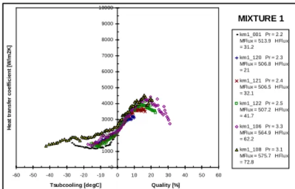
The second case of departure from the classical behaviour of convective boiling heat transfer is the deterioration of heat transfer coefficient with increasing quality at (high) qualities typical of annular flow. The heat transfer coefficient behaviour as a function of quality is shown in Figure 8 (Kandlbinder, 1997). Similar behaviour was observed by many investigators for a number of binary and multicomponent mixtures in both vertical (Celata et al., 1994; Shatto, 1998) and horizontal systems (Wettermann and Steiner, 2000). An extensive literature review was carried out by Barbosa (2001).
In binary and multicomponent evaporating systems, the difference in volatility between the components gives rise to axial gradients of concentration (and hence of saturation temperature) in both liquid and vapour streams due to the preferential evaporation of the more volatile component(s) even when local component equilibrium occurs. Figure 9, adapted from Thome and Shock
(1984), illustrates the axial distributions of saturation and wall temperature for a mixture and for a single component undergoing phase change in a tube. As quality increases, the liquid phase becomes richer in the less volatile component and the fluid saturation temperature increases (in many cases, overcoming the decrease associated with the negative axial pressure gradient).
MIXTURE 1
0 1000 2000 3000 4000 5000 6000 7000 8000 9000 10000
-60 -50 -40 -30 -20 -10 0 10 20 30 40 50 60
Tsubcooling [degC] Quality [%]
H
e
a
t
tr
a
n
s
fe
r
c
o
e
ff
ic
ie
n
t
[W
/m
2
K
]
km1_001 Pr = 2.2 MFlux = 513.9 HFlux = 31.2 km1_120 Pr = 2.3 MFlux = 506.8 HFlux = 21 km1_121 Pr = 2.4 MFlux = 506.5 HFlux = 32.1 km1_122 Pr = 2.5 MFlux = 507.2 HFlux = 41.7 km1_106 Pr = 3.3 MFlux = 564.9 HFlux = 62.2 km1_108 Pr = 3.1 MFlux = 575.7 HFlux = 72.8
Figure 8. Heat transfer coefficient as a function of the equilibrium quality (saturated region) and of subcooling (subcooled region) in flow boiling of 70% n-pentane, 30% iso-octane (molar basis) (Kandlbinder, 1997).
Distance, z
T
e
m
p
e
ra
tu
re
,
T
pure fluids
mixtures
w T
b T
w T
sat
b T
T=
sat
b T
T=
w T
w T dryout
Distance, z
T
e
m
p
e
ra
tu
re
,
T
pure fluids
mixtures
w T
b T
w T
sat
b T
T=
sat
b T
T=
w T
w T dryout
Figure 9. Temperature profiles and boiling regimes for convective evaporation (Thome and Shock, 1984).
In the annular flow regime, without bubble nucleation at the wall, the heat transfer coefficient decrease associated with mixture effects takes place in different ways depending on the form of heating imposed to the surface (Wadekar, 1990). In the present context, mixture effects are defined as the build-up of concentration gradients adjacent to the vapour-liquid interface resulting from the preferential evaporation of the more volatile component(s). This decreases the interfacial concentration of the lighter component, ~ , xI to a value lower than the bulk liquid phase concentration, ~ . For xb
simplicity, ideal cases in which no droplet interchange (entrainment) exists are depicted in Figures 10.a and 10.b. These figures exhibit temperature profiles across the liquid film for prescribed wall temperature and heat flux boundary conditions, respectively. In both cases, profiles with and without mixture effects are shown.
interface interface
with mixture effect
without mixture effect with mixture
effect without mixture effect
'
w
T
w
T
wT
( )
I bubI T x
T = ~
( )
I bubI T x
T = ~
( )
b bubI T x
T = ~ TI Tbub
( )
xb~ =
(a) (b)
interface interface
with mixture effect
without mixture effect with mixture
effect without mixture effect
'
w
T
w
T
wT
( )
I bubI T x
T = ~
( )
I bubI T x
T = ~
( )
b bubI T x
T = ~ TI Tbub
( )
xb~ =
(a) (b)
In the wall temperature controlled case (Figure 10.a), the decrease in the heat transfer coefficient calculated according to Eq. (1) is due to the reduction in the temperature driving force is from
( )
b bubw T x
T − ~ to Tw−Tbub
( )
x~I . In the heat flux controlled case, the rise in the interface temperature does not change the temperature driving force. Rather, this potential must remain unchanged so that the product of the local (film) heat transfer coefficient and thetemperature difference is equal to the applied heat flux2. The
increase in wall temperature from T to w Tw′ is illustrated in Figure 10.b.
So what causes the reduction of the heat transfer coefficient observed so systematically in the literature for the constant heat flux case? The answer is practicality. For engineering design
calculations, it is more convenient to define α in terms of
( )
b bubw T x
T′− ~ than Tw′ −Tbub
( )
~xI , where Tw′ is generallydetermined experimentally. Because Tbub
( )
x~b is lower than( )
I bub xT ~ , the ratio of the wall heat flux to the design based wall superheat is also lower. It is therefore expected that conventional prediction methods that do not take these effects into account will overestimate the experimental heat transfer coefficient.
As will be shown in Section 5, in order to properly quantify Tw′
and Tbub
( )
~xb in the annular flow regime and consequently predict the heat transfer coefficient under forced convective boiling, two mechanisms must be accounted for, namely,a. Mass transfer resistance as a result of component(s)
preferential evaporation and formation of concentration gradients adjacent to phase interface(s) in both phases;
b. A hydrodynamic non-equilibrium resulting from the
difference in average concentration between the liquid film and the liquid entrained as droplets in the gas core.
Item b above is a direct consequence of the processes of droplet entrainment and deposition; vigorous mass exchange phenomena which disrupt the hydrodynamic equilibrium of annular flow. Amongst other effects, these phenomena are known to exert a large influence on important flow parameters like pressure drop (Hewitt and Hall-Taylor, 1970). Nevertheless, the significance of droplet interchange on forced convective boiling of mixtures seems to have been overlooked in previous studies and the correct prediction of this mechanism may hold the key to understanding the deterioration associated with the heat transfer coefficient at high qualities (Barbosa and Hewitt, 2001a, 2001b; Barbosa et al., 2002a, 2002b).
Figure 11 depicts an interpretation of the physics of the mixture vaporization problem. In design calculations, the two-phase flow pattern is usually ignored and it is implicitly assumed that the whole of the liquid flow is available for evaporation (Figure 11.b). Usually, a flash calculation is used to determine the amount of liquid which has evaporated for a given wall heat flux and the saturation (bubble point) temperature of the mixture. The preferential evaporation of the more volatile component gives rise to axial gradients of saturation temperature and of mean concentration in both phases.
In a real situation, however, where the annular flow pattern is the dominant configuration, not all of the liquid is present as a film coating the inner wall of the pipe. Rather, droplets are generated from the crests of disturbance waves which travel along the liquid film and these droplets become entrained in the vapour core (Figure 11.a). The droplets travel at approximately the same velocity as the
2 It is implicitly assumed that the liquid film heat transfer coefficient is independent of mixture effects. The validity ofsuch a hypothesis was discussed by Shock (1976).
vapour. All along the channel, droplets are being exchanged between the film and the core by entrainment and deposition. However, this exchange is not rapid enough to maintain equality of composition between the droplets and the film. Bearing in mind that droplet evaporation may be negligible when compared to that of the liquid film (the temperature driving force in the liquid film is much higher), one can argue that in the actual situation not all of the liquid phase will be available for evaporation at a given distance along the pipe. This hydrodynamic effect breaks down the thermodynamic equilibrium relationship existing between quality and mixture saturation temperature.
For the sake of clarity, let us consider first the simplified situation in which a certain amount of liquid is entrained as droplets at the onset of annular flow and in which no further entrainment or deposition occurs downstream of this point. In this case, the initial film flow rate (amount of liquid initially available for evaporation) is equal to the total liquid flow rate less the initial entrained droplet flow rate. Even in this ideal situation where the entrained liquid flow is disregarded in the thermodynamic calculation, vapour-liquid equilibrium still demands that a fixed amount of liquid must be lost by evaporation for a given wall heat flux and, at the point of film depletion (‘dryout’), the film (saturation) temperature must be equal to the dew point temperature at the overall composition. Since the film flow rate is less than the total liquid flow rate, then (a) ‘dryout’ will occur at a shorter distance along the channel than it would if all the liquid were in the film, and (b) the film saturation temperature at a given position will be higher than the saturation temperature calculated for a case in which all the liquid flow is considered in the thermodynamic calculations.
HIGH Actual situation
Concentration of more volatile component LOW
Implicitly assumed in design
(a) (b)
HIGH Actual situation
Concentration of more volatile component LOW
Implicitly assumed in design
(a) (b)
Actual situation
Concentration of more volatile component LOW
Implicitly assumed in design
Implicitly assumed in design
(a) (b)
Figure 11. Liquid phase distribution in annular flow of binary and multicomponent mixtures.
simplified ‘no interchange’ approach for each initial entrained fraction.
In the forced convective region (absence of nucleate boiling),
the liquid film heat transfer coefficient is primarily a function of
local turbulence and of physical properties. In general, however, the temperature change in the liquid film is dominated by that occurring in the region near the wall where the flow is laminar and turbulence is suppressed. Between this near-wall zone and the interface, the temperature changes little due to the mixing caused by turbulence. This same mixing process in the film leads to a situation where the component concentrations in the liquid film are relatively constant and the interface concentration is close to the mean (fully mixed) concentration in the liquid film. This result was demonstrated quantitatively by Shock (1976), who showed that for any mixture, irrespective of the width of its boiling range, the effect of mass
transfer in the liquid film is small enough to be ignored; that is, the
interface concentration is close to that of the fully mixed film. Shock (1976) also investigated the influence of mass transfer in the vapour core. He found that the effects were more significant than those for the liquid film (though still small). The vapour created by evaporation at the interface has to be transported through a laminar-like layer in the vapour adjacent to the interface. This transport process is achieved by a flow normal to the interface coupled with diffusive mass transfer, the latter depending on the concentration gradient of the components. In the work described in this lecture, these mass transfer processes have been considered in detail. It transpires that their effect is small compared to the drop/film concentration difference effect mentioned above, though they could become significant in some circumstances.
Thermodynamic Non-Equilibrium Slug Flow
Governing Equations
The model is based on a succession of slug units consisting of a Taylor bubble (formed as a result of the abrupt vapour growth in the subcooled region) surrounded by a falling liquid film and a liquid slug (Figure 12). Due to the formation of the vapour plugs in the subcooled bulk region, it is postulated that the liquid slugs are initially subcooled. Additional simplifications are proposed: (i) a substantial portion of the energy associated with the high temperatures in the near-wall region is consumed in the process of generation of the Taylor bubble and therefore the falling film is assumed saturated, (ii) phase change in the liquid slug and slug body gas hold-up are negligible, (iii) the thickness of the liquid film surrounding the Taylor bubble is small compared with the pipe diameter, (iv) the mass of the liquid film is small compared with that of the slug, (v) phase densities are constant within the slug unit, and (vi) the rate of change of the Taylor bubble length with time is small compared with the ascension velocity of the Taylor bubble. Energy balances over the slug unit and the over the liquid slug give (Barbosa and Hewitt, 2004),
(
)
− + =
dz T d L c V
d L L q h dz
dL S
S pL L GB T
S B w v G
B ρ
∆ ρ
4 1
, (4)
(
)
+
− =
GB T L
S B w S S pL v S
V d
L L q dz T d L c h dz dL
ρ ∆
4 1
, (5)
(
sat S)
B S L G LS pL L
w T S
T T dz dL L V
c q d dz T d
− −
= 4 1
ρ ρ
ρ , (6)
where LBand LSare the lengths of the Taylor bubble and of the
liquid slug regions, T is the average temperature of the liquid slug, S
GB
V and VLS are the velocities of the centre of mass of the Taylor
bubble and of the liquid slug, respectively.
b
L
s
L
G B
V
L B
V
L S
V g
z
G S
V
b
L
s
L
G B
V
L B
V
L S
V g
z
b
L
s
L
G B
V
L B
V
L S
V g
z
G S
V
Taylor Bubble
Liquid Slug
b
L
s
L
G B
V
L B
V
L S
V g
z
G S
V
b
L
s
L
G B
V
L B
V
L S
V g
z
b
L
s
L
G B
V
L B
V
L S
V g
z
G S
V
Taylor Bubble
Liquid Slug
Figure 12. Geometry of a slug unit.
To close the model, the above equations are combined with mass conservation relationships borrowed from steady-state slug flow models (Fernandes et al., 1983; Orell and Rembrand, 1986; Sylvester, 1987; De Cachard and Delhaye, 1996).
GB B
GS V
U =βε , (7)
(
B)
LB M GBBV + −ε V =U
ε 1 , (8)
(
)
[
G L G G]
LS GS M
LS U U U G x x
V = = + = 1− ρ + ρ , (9)
0 2 .
1 U V
VGB= M + , (10)
where UM is the mixture velocity. The rise velocity of a Taylor
bubble in a quiescent liquid, V , and the falling film velocity, 0 VLB,
are obtained through empirical relationships provided by Wallis (1969).
The model equations are solved so that at each step z∆ , a value
of β (defined as the ratio of the Taylor bubble length to the length
of the slug unit) is calculated together with the real quality,x , and G
the remaining slug flow parameters. It is postulated that the onset of slug flow is associated with the point at which vapour is initially formed and the correlation of Saha and Zuber (1974) for the Point of Net Vapour Generation (NVG) is used to calculate the distance from the liquid inlet up to the point of initiation of slug flow. The model of Saha and Zuber also provides the liquid slug temperature at the onset of slug flow. A thorough discussion concerning the determination of the initial conditions for the Taylor bubble and liquid slug lengths is given elsewhere (Barbosa and Hewitt, 2004).
Heat Transfer
In slug flow, the local time averaged wall temperature to be used in Eq. (1) is defined as (Barnea and Yacoub, 1983),
(
sf wf ss wS)
wf(
)
wSsp
ss t sf t
sf t
w sf
t w sp sp
t w sp w
T T
T t T t t
dt T dt T t dt T t T
, ,
, ,
0 0
1 1
1 1
β
β + −
= +
=
∫
+
∫
=
∫
= +
In the liquid slug and in the Taylor bubble regions, superposition models for forced convective boiling (Chen, 1966) were used to determine the local time-averaged wall temperatures. These are as follows (note that slug body subcooling is assumed),
S nb S fc
sat S nb S S fc w S w
T T
q T
, ,
, ,
, α α
α α
+ + +
= , (12)
f nb f fc
w sat
f w
q T
T
, ,
, = +α +α . (13)
The forced convective terms of the heat transfer coefficients in the falling film and slug regions, αfc,f and αfc,S were calculated
using the Chun and Seban (1971) correlation and the Chen (1966) model modified according to Butterworth and Shock (1982) to deal
with subcooling effects. The nucleate boiling terms αnb,f and
S nb,
α were calculated according to the Chen (1996) model.
Results
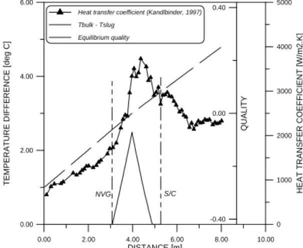
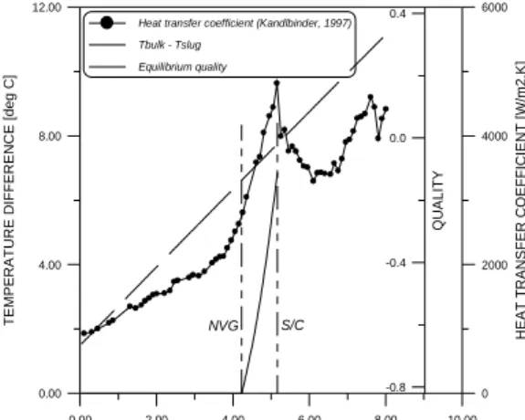
The experimental heat transfer coefficient behaviour, together with the difference between the slug temperature and the equilibrium bulk temperature is shown in Figure 13 for a typical n-pentane boiling run. In this case, the temperature difference
increases from zero up to 3oC at the point whereTb=Tsat and then
starts to decrease. T is the local equilibrium bulk temperature and b
sat
T is the local saturation temperature. Two vertical lines in Figure
13 define the portion of the flow in which the slug flow pattern prevails according to the model. The line upstream of the peak represents the NVG Point (Saha and Zuber, 1974) and the line downstream of the peak marks the transition to churn flow according to the model of Jayanti and Hewitt (1992). In this figure, a coincidence is observed in the locations of the regions of maxima in the Tb−TS and in the heat transfer coefficient profiles. This fact
was observed consistently in the simulations (as can be seen from two examples in Figures 14 and 15) and is crucial to understanding the model’s ability to predict the heat transfer coefficient peaks in the near-zero quality region.
0.00 2.00 4.00 6.00 8.00 10.00
DISTANCE [m] 0.00
2.00 4.00 6.00 8.00
T
E
M
P
E
R
A
T
U
R
E
D
IF
F
E
R
E
N
C
E
[
d
e
g
C
]
0 2000 4000 6000 8000
H
E
A
T
T
R
A
N
S
F
E
R
C
O
E
F
F
IC
IE
N
T
[
W
/m
2
.K
]
-0.4 0.0 0.4
Q
U
A
L
IT
Y
Heat transfer coefficient (Kandlbinder, 1997)
Tbulk - Tslug
Equilibrium quality
S/C NVG
Figure 13. Slug to equilibrium bulk temperature difference as a function of
distance. N-pentane, inlet pressure: 4.9 bar, total mass flux: 376.0 kg/m2s,
wal heat flux 50.0 kW/m2, inlet temperature: 60.7 oC.
A bubble that nucleates adjacent to the wall may grow sufficiently to form a vapour plug and induce an early transition to
churn flow in the subcooled bulk region. As this bubble continues to grow, it accelerates the liquid slug ahead of it, thus reducing the residence time of the liquid slug in the pipe. With their residence times reduced, the liquid slugs will remain subcooled at greater distances along the pipe where, according to the thermodynamic equilibrium hypothesis, they should be saturated. As a result, at a given distance, the real quality (and consequently the heat transfer coefficient, because of a lower time-averaged wall temperature) will be higher than that calculated assuming thermodynamic equilibrium.
0.00 2.00 4.00 6.00 8.00 10.00
DISTANCE [m] 0.00
2.00 4.00 6.00
T
E
M
P
E
R
A
T
U
R
E
D
IF
F
E
R
E
N
C
E
[
d
e
g
C
]
-0.40 0.00 0.40
Q
U
A
L
IT
Y
0 1000 2000 3000 4000 5000
H
E
A
T
T
R
A
N
S
F
E
R
C
O
E
F
F
IC
IE
N
T
[
W
/m
2
.K
]
NVG S/C
Heat transfer coefficient (Kandlbinder, 1997)
Tbulk - Tslug
Equilibrium quality
Figure 14. Slug to equilibrium bulk temperature difference as a function of
distance. Iso-octane, inlet pressure: 3.1 bar, total mass flux: 200.8 kg/m2s,
wal heat flux 19.5 kW/m2, inlet temperature: 117.4 oC.
As can be seen from the slug temperature profiles shown in Figures 16 and 17, since the liquid slug velocity increases continuously as a result of acceleration of the Taylor bubble, the subcooling reduction is much less pronounced as a function of distance than what would be the case under thermodynamic equilibrium. In addition, Figures 13-15 show that as the transition to churn flow is approached (S/C) there is a decrease in the heat transfer coefficient to values typical of those normally associated with the classical behaviour (Collier and Thome, 1994; Hewitt, 2000). Since the slug-to-churn flow transition is triggered by the collapse of the slug unit, the resulting homogenization of the phases in the Taylor bubble region and in the liquid slug would eliminate the local subcooling effects responsible for maintaining the local heat transfer enhancement. This phenomenon is most visible in Figures 15 and 17.
The ability of the methodology to predict the local heat transfer coefficient behaviour is illustrated in Figures 18 and 19 for typical n-pentane and iso-octane runs. In both cases, the experimental data trends are well predicted upstream and downstream of the saturation point (marked by “X”). As a result of the calculated peaks in the
S b T
T − profiles, the zones of higher calculated heat transfer
coefficients also coincide with the experimental ones.
maxima in the heat transfer coefficient profiles. The general performance of the model over a representative range of the database of Kandlbinder (1997) is presented in Figure 20, where 95% of the non-equilibrium model data lies in the +/- 18% relative error band.
0.00 2.00 4.00 6.00 8.00 10.00
0 2000 4000 6000
H
E
A
T
T
R
A
N
S
F
E
R
C
O
E
F
F
IC
IE
N
T
[
W
/m
2
.K
]
-0.8 -0.4 0.0 0.4
Q
U
A
L
IT
Y
0.00 4.00 8.00 12.00
T
E
M
P
E
R
A
T
U
R
E
D
IF
F
E
R
E
N
C
E
[
d
e
g
C
]
NVG S/C
Heat transfer coefficient (Kandlbinder, 1997)
Tbulk - Tslug
Equilibrium quality
Figure 15. Slug to equilibrium bulk temperature difference as a function of
distance. Iso-octane, inlet pressure: 2.2 bar, total mass flux: 296.7 kg/m2s,
wal heat flux 60.1 kW/m2, inlet temperature: 55.3 oC.
0.00 2.00 4.00 6.00 8.00 10.00
DISTANCE [m] 60.00
70.00 80.00 90.00 100.00 110.00
T
E
M
P
E
R
A
T
U
R
E
[
K
]
NVG (theoretical)
Experimental (Kandlbinder, 1997)
Saturation temperature
Equilibrium bulk temperature
Slug temperature
Figure 16. Axial temperature profiles (measured at the centreline – Kandlbinder, 1997). N-pentane, inlet pressure: 6.0 bar, mass flux: 377.4
kg/m2s, wall heat flux: 49.9 kW/m2, inlet temperature: 67.5 oC.
0.00 2.00 4.00 6.00 8.00 10.00
DISTANCE [m] 40.00
80.00 120.00 160.00
T
E
M
P
E
R
A
T
U
R
E
[
d
e
g
C
]
NVG (theoretical)
S/C
Experimental (Kandlbinder, 1997)
Saturation temperature
Equilibrium bulk temperature
Slug temperature
Figure 17. Axial temperature profiles (measured at the centreline – Kandlbinder, 1997). Iso-octane, inlet pressure: 2.2 bar, total mass flux:
296.7 kg/m2s, wall heat flux: 60.1 kW/m2, inlet temperature: 55.3 oC.
3.20 3.60 4.00 4.40 4.80 5.20
DISTANCE [m] 2000
4000 6000 8000
H
E
A
T
T
R
A
N
S
F
E
R
C
O
E
F
F
IC
IE
N
T
[
W
/m
2
.K
]
Experimental (Kandlbinder, 1997)
Present model (Non-equilibrium slug flow)
Chen (1966)
X
Figure 18. Local heat transfer coefficient prediction. N-pentane, inlet
pressure: 6.0 bar, total mass flux: 377.4 kg/m2s, total heat flux: 49.9
kW/m2, inlet temperature: 67.5 oC.
3.00 3.50 4.00 4.50 5.00 5.50
DISTANCE [m] 1000
2000 3000 4000 5000 6000
H
E
A
T
T
R
A
N
S
F
E
R
C
O
E
F
F
IC
IE
N
T
[
W
/m
2
.K
]
Experimental (Kandlbinder, 1997)
Present model (Non-equilibrium slug flow)
Chen (1966)
X
Figure 19. Local heat transfer coefficient prediction. Iso-octane, inlet
pressure: 3.1 bar, total mass flux: 200.8 kg/m2s, total heat flux: 19.5
kW/m2, inlet temperature: 117.4 oC.
0 2000 4000 6000 8000
EXPERIMENTAL HEAT TRANSFER COEFFICIENT [W/m2.K] 0
2000 4000 6000 8000
C
A
L
C
U
L
A
T
E
D
H
E
A
T
T
R
A
N
S
F
E
R
C
O
E
F
F
IC
IE
N
T
[
W
/m
2
.K
]
Present model (Non-equilibrium slug flow)
Chen (1966)
-18% +18%
Figure 20. Comparison between experimental and calculated local heat transfer coefficients.
Annular Flow of Binary and Multicomponent Mixtures
Hydrodynamics
annular flow takes place. The mass flow rates per unit cross-sectional area, m, of the three fields, viz., liquid film, LF, vapour core, GC, and entrained liquid, LE, are shown. The initial bulk concentrations (in terms of mass fractions) of the ith component in the liquid film, entrained droplets and vapour core arex0LF,i, x0LE,i
and yGC0 ,i, respectively. An initial value is assumed for the fraction of liquid entrained as droplets at the point of initiation of the annular regime and the concentration of the respective components in this initially entrained liquid is assumed equal (at this point) to that of the liquid film (though differences develop later). The transition to annular flow is determined by the critical velocity criterion for flow reversal due to Wallis (1969).
The number of droplets depositing per unit time per unit area of tube wall at section m is defined by the cumulative operator as follows,
∑
= = m j
m j D m
D n
n 0
,
, (14)
where, nDj,m is the number of droplets per unit time per unit area of tube wall that were entrained at a section j (lower than m) and that
deposit at section m. Analogously, nmE is defined as the number of
droplets per unit time per unit area of tube wall that were entrained at section m. If the entrainment and deposition rates at any point in
the channel are known, then nDj,mand nmE are given by,
m pc m m E
M E
n = , (15)
and,
m j p m j m j D
M D
n ,
,
, =
, (16)
where E and D are rates of droplet entrainment and deposition and
M is the mass of a droplet. Subscripts pand pcstand for droplet
and droplet at the moment of creation, respectively.
xLF i,,xLE i,,y ,i
3 3 3
GC
Liquid film
g
z m = 0
m = 1 m = 2 m = M
m = 3
xLF i,,xLE i,,y ,i
0 0 0
GC
xLF i,,xLE i,,y ,i
1 1 1 GC
x x y
LF i M
LE M
i M
,, ,GC,
x x y
LF i m
LE m
i m
,, , GC,
Entrained
droplet Vapourcore
xLF i,,xLE i,,y ,i
2 2 2
GC
Concentration of more volatile component
LOW HIGH
Figure 21. A schematic of the annular flow model.
Droplets were assumed spherical and droplet diameters at creation were calculated through the correlation of Azzopardi et al.
(1980). The entrainment and deposition rates, EmandDj,mwere
determined through a modification of the set of correlations developed by Govan et al. (1988). A more detailed description of the liquid phase mass interchange between the liquid film and the entrained droplets is given in Barbosa and Hewitt (2001a).
The following differential equations are obtained through mass
balances over an element of tube of length dzfor a mixture of NOC
components. Equations (17) to (19) represent overall mass conservation for the liquid film, vapour core and liquid entrained as droplets. Equation (20) is a component mass balance for the liquid film. The effect of deposition of droplets having different concentrations is characterised by the expression in parenthesis in the RHS of Eq. (20).
(
− −∑)
= NOC=
j I j
T
LF D E m
d m dz
d
1 ,
4
, (17)
∑
= NOC=
j I j
T
GC m
d m dz
d
1 ,
4
, (18)
(
E D)
d m dz
d
T
LE= −
4
, (19)
(
)
[
LFi LFi NOCj I j LFi Ii]
LF T i
LF Dx Dx m x m
m d x dz
d
,
1 , ,
, ,
,
4 − +∑ −
= = . (20)
i I
m,is the mass flux of component i in the evaporating stream,
calculated through a model for simultaneous interfacial heat and mass transfer based on a film (or Colburn) method in which the effect of droplet interchange is taken into account in the interfacial heat balance (see Section 5.2). An energy balance over an element of length dz gives,
(
)
(
)
(
)
[
GC I C pLE I C]
pC C T
C T T E D c T T
c m d T dz
d = 4 α• − + − −
, (21)
where the subscript Crepresents the homogeneous core properties
and αGC• is the finite-flux gas core heat transfer coefficient (Bird et al., 1960). The momentum conservation and additional closure relationships for hydrodynamics were obtained from an annular flow modelling framework (Hawkes, 1996; Barbosa, 2001) in which the triangular relationship between film thickness, film flow rate and interfacial shear stress is invoked together with the relationships for entrainment and deposition rates.
Heat and Mass Transfer
At each integration step z∆ , an iterative procedure is carried out
to determine the interfacial mass fluxes, compositions and temperature. Classically, the film interface condition can be determined by either assuming full or no mixing in the liquid film. For the present geometry and flow regime in the liquid film, the fully mixed liquid determinacy condition seems more appropriate. In this case, the interfacial liquid composition is known a priori (i.e., it is equal to the mean film composition) and a bubble point calculation defines the interfacial state. The solution algorithm for the interphase heat and mass transfer calculation is as follows (Webb, 1982),
2. Calculate: yI,i,TI→ Bubble point temperature subroutine;
3. Guess: ∑NOC=
j 1 mI,j;
4. Calculate: ∑NOC=
j I j
j
I m
m , 1 , → Eq. (26);
5. Calculate: qGC → Eq. (22);
6. Compare: If qGC≠qW−qED, update ∑NOCj=1 mI,jand return
to step 4.
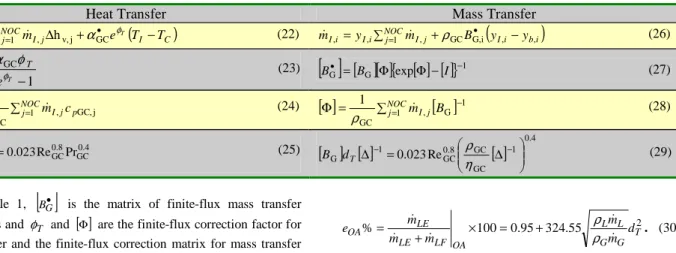
The relationships utilized in the interfacial heat and mass iterative balances are summarized in Table 1. The elements of the
diagonal matrix of diffusion coefficients,
[ ]
∆ , are determinedthrough an Effective Diffusivity approach or through and Interactive Method (Taylor and Krishna, 1993). In either case, Maxwell-Stefan diffusion coefficients for the gas phase were calculated assuming
ideal gas behaviour using the correlation of Fuller et al. (1964). For additional details concerning the interphase heat and mass transfer formulation, see Barbosa et al. (2002a).
Step 6 of the iterative algorithm assumes qGC=qw−qED,
whereqED=
(
E− D)
cpLE(
TI−TC)
is the energy released/absorbedby the entrained droplets due to entrainment and deposition. Finally,
the time-averaged wall temperature, TW, is given by
LF W I
W T q
T = + α , where αLFis the heat transfer coefficient for
the liquid film calculated using the correlation of Chen (1966) with the (small) nucleate boiling component corrected for mixture effects as suggested by Palen (1992).
Table 1. Summary of interfacial balance equations.
Heat Transfer Mass Transfer
(
I C)
NOC
j mI j e T T
q =∑ ∆ + • T −
=1 , v,j αGC φ
GC h (22) mI,i=yI,i∑NOCj=1 mI,j+ρGCBG,i•
(
yI,i−yb,i)
(26)1 GC GC
− =
•
T
e T
φ
φ α
α (23)
[ ]
[ ][ ] [ ] [ ]
{
}
1 GG• = B Φ expΦ− I −
B (27)
∑
= NOC=
j Ij p
T 1 m, c GC,j
GC 1
α
φ (24)
[ ]
[ ]
1G
1 ,
GC
1 −
=
∑
=
Φ NOCm B
j Ij
ρ (28)
0.4 GC 0.8 GC GC
GC =0.023Re Pr
λ
α dT (25)
[ ] [ ]
[ ]
4 . 0 1
GC GC 8 . 0 GC 1
G 0.023Re
∆ =
∆− −
η ρ
T
d
B (29)
In Table 1,
[ ]
BG• is the matrix of finite-flux mass transfercoefficients and φT and
[ ]
Φ are the finite-flux correction factor forheat transfer and the finite-flux correction matrix for mass transfer (Bird et al., 1960).
The Effect of Initial Entrained Fraction
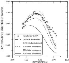
In single component systems, the modelling work of Govan (1990) showed that the behaviour of thermal parameters such as the local heat transfer coefficient and the critical heat flux are affected only slightly by the fraction of the total liquid flow entrained as droplets at the onset of annular flow. On the other hand, it has been shown that for annular flow of binary (Barbosa and Hewitt, 2001a, 2001b) and of ternary mixtures (Barbosa and Hewitt, 1999; Barbosa et al., 2002a) significant discrepancies may develop between profiles of local heat transfer coefficient calculated using different (hypothetical, but within a realistic range; say, from 0% to 40%) initial entrained liquid fractions. These discrepancies arise as the initial entrained fraction affects the downstream distribution of the components between the drops and the liquid film, giving rise to the hydrodynamic non-equilibrium phenomenon described in Section 3.1. It is, therefore, essential that appropriate boundary conditions for the initial entrained fraction are provided in order to solve the heat and mass transfer in flow boiling of mixtures at high qualities.
An empirical correlation was developed (Barbosa et al., 2002c) to calculate the fraction of the total liquid flow entrained as droplets at the region of transition between the churn flow and the annular flow regimes. Measurements of local gas and entrained liquid mass fluxes were carried out using an isokinetic probe system. Amongst other findings, it was observed that in the fully co-current annular flow region local droplet concentration is virtually constant within the gas core. In contrast, the churn flow regime exhibits rather sharp radial gradients of concentration which gradually disappear with increasing gas velocity. The correlation is as follows,
2 55
. 324 95 . 0 100
% T
G G
L L OA
LF LE
LE
OA d
m m m
m m e
ρρ
+ = × +
= . (30)
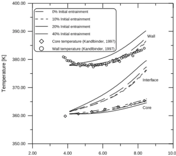
Equation 30 was used to compute the entrained fraction in adiabatic air-water systems and was also incorporated into the binary and multicomponent annular flow boiling calculation framework (Barbosa et al., 2002b). As will be seen in Section 5.4, a comparison of local wall temperature profiles and local and average heat transfer coefficients for flow boiling of binary and ternary hydrocarbon mixtures (Kandlbinder, 1997) reveals an encouraging agreement between the theory and the experimental data.
Results
The model predictions were extensively compared with the experimental database of Kandlbinder (1997) for forced convective boiling experiments of pure hydrocarbons (n-pentane, n-hexane and iso-octane) and their mixtures in an 8.68 m long, vertical 321 stainless steel tube test section. The inner and outer diameters were 25.4 and 38.0 mm, respectively. Along the test section, bulk fluid (centreline) and wall temperatures were measured.