J. Padet
UTAP – Laboratoire de Thermomécanique, Faculté des Sciences B.P. 1039, 51687 REIMS, France [email protected]
Transient Convective Heat Transfer
In nature, as well as within the human-made thermal systems, the time-variable regimes are more commonly encountered, if not always, than the permanent regimes. Nevertheless, studies in convection are still more frequent in the permanent regimes, undoubtedly due to the related difficulties in calculation in terms of time and cost of computation.
One may distinguish two categories of time-dependent transfers: those which are due to external causes (variable boundary conditions) and those that are due to internal causes (sources of variable power, instabilities, turbulence), and the combination of these two types may also be encountered.
In this presentation, we shall analyze some situations which belong to the first category. These are concerned with:
− a group of boundary layer flows in forced, natural or mixed convection, where the wall is subjected to time-variable conditions in temperature or flux.
− another group of fluid flows within ducts, in laminar mixed convection regime, where the entry conditions (mass flow rate, temperature) are time-dependent.
The techniques of analysis are mainly extensions to the differential method and to the integral method of Karman-Polhausen in boundary layer flows, and the finite differences solution of the vorticity and energy equations for internal flows.
The results presented in the transient state are caused by steps of temperature, heat flux or velocity, and in particular show the time evolution of the dynamic and thermal boundary layers, as well of the heat transfer coefficients.
Three examples of applications will then be treated: the active control of convective transfers, the measurement of heat transfer coefficients, and the analysis of heat exchangers.
The main idea in the active control is that of managing the temperatures or heat fluxes by employing a variable regime. Under certain conditions, this procedure may reveal itself quite interesting.
The measurement of transfer coefficients by the photothermal impulse method possesses a great interest since it is performed in a non-intrusive way without contact. However, in order to be precise, it needs to account for the thermal boundary layer perturbation due to the radiative flux sent over the surface, which means to know the evolution of the transfer coefficient during the measurement. Previous studies therefore provide essential information.
Within the domain of heat exchangers, we shall present a different global method, which allows for the evaluation of the time constant of an equipment in response to sample variations of temperature or mass flow rates at the entrance.
In conclusion, a brief balance of the ICHMT Symposium “Transient heat and mass transfer”, Cesme, Turkey, August 2003, will be presented.
Keywords: Transient, heat transfer.
Introduction
Transient convection is of fundamental interest in many industrial and environmental situations such as air conditioning systems, human comfort in buildings, atmospheric flows, motors, thermal regulation process, cooling of electronic devices, security of energy systems… Many works reported in literature deal with stationary velocity and temperature fields, but only a small number deal with time – variable boundary conditions [1, 2, 3, 4], either in forced, natural or mixed convection.1
In this lecture, we intend to complete previous analysis and to introduce researches about transient convection realised at the UTAP-LTM laboratory in Reims.
Forced Convection
Description of the Problem
The aim of this first part is to present a detailed numerical study of the transient forced laminar convective heat transfer over a flat
Presented at ENCIT2004 – 10th Brazilian Congress of Thermal Sciences and Engineering, Nov. 29 -- Dec. 03, 2004, Rio de Janeiro, RJ, Brazil.
Technical Editor: Atila P. Silva Freire.
plate or a wedge, when the thermal field is due to different kinds of variations – in time and space – of some boundary conditions, i.e. wall temperature or wall heat flux. The governing equations are solved using extensions either of the differential method, or the Karman – Pohlhausen integral approach. Let precise that in this whole part, we consider uncoupled situations, i.e. the velocity field does not depend on the thermal field.
T(x,y,t)
δ
Tp(x,y,t)
δt
. const qext=
x y
e(t) E
∞ ∞T U ,
∞ U
∞ T
T0(x,t)
Figure 2.1. Representation of the physical model.
Plate with No Thickness
Differential Method [5] [6] [7]
First introduce as an example transient laminar forced convection from a wedge subjected to a positive step change in its surface temperature. At time t < 0, a flow is deflected through an angle
β
π
/2 between the x-direction on the wedge surface and the direction of flow. The coefficient β is defined as: β = 2m / (m + 1), where m is the pressure-gradient parameter along the x-direction, so that U∞(x) = C xm, where C is a constant. Of course, the special case m = 0 describes the flow on a flat plate without pressure gradient. Initially, the flow and the surface wedge are both at the same temperature, T∞. At time t = 0, the surface temperature of the wedge is changed to the value Tp and subsequently held constant, thereforesetting up a time-dependent thermal boundary layer.
βπ
βπ
βπ
βπ
x
0
U
∞∞∞∞= C
x
mβπ
βπ
βπ
βπ
x
0
U
∞∞∞∞= C
x
mFigure 2.2. Flow over a wedge.
The partial differential equations that describe the problem are:
0 = + y V x U ∂ ∂ ∂ ∂ 2 2 1 y U x d p d y U V x U U ∂ ∂ ν ρ ∂ ∂ ∂ ∂ + =− + 2 2 y T a y T V x T U t T ∂ ∂ ∂ ∂ ∂ ∂ ∂ ∂ + + =
The boundary conditions are as follows:
∞ ∞ ∞ = = ∞ = = T ) t , , x ( T ) x ( U ) , x ( U ) , x ( V ) , x ( U and : stream free the in 0 0 0 : surface the at
and the initial conditions:
p T ) t , , x ( T : t ; T ) t , y , x ( T :
t=0 = ∞ ≥0 0 =
Defining the dimensionless quantities:
∞ = U / x y ν
η , t
x U
t+= ∞ , and
∞ ∞ + − − = = T T T T ) t , ( T T p * * η
the velocity components in x and y directions are expressed as follows: ) ( ' F U
U = ∞ η
(
F' (m )F)
xU
V 1
2
1 − +
= ∞ν η
where ‘prime’ denotes the differentiation with respect to η.
By introduction of the transformation variables in the momentum equation, the dimensionless stream function, F (η), verifies the known Falkner-Skan equation:
(
1)
02
1 + − 2 =
+
+m FF' m F'
' ' ' F
For a sudden change in the wedge temperature, we show that the dimensionless quantities η, t+ and T* verifie the differential equation:
[
]
− + = + + + + t T t ' F ) m ( ' FT m ' ' T Pr * * * ∂ ∂ 1 1 2 1 1with the boundary and initial conditions:
1 0
0 = =∞ =
= ) ; F'( )
( '
F η η
0 ) , ( and 1 ) , 0 ( ; 0 0 ) , ( ; 0 * * * = ∞ = ≥ = = + + + + + t T t T t t T t η
The gradient-pressure parameter m can be positive or negative; negative values are encountered, for example, near the rear of a wedge. For attached boundary layers, the solutions of equation (7) are limited to values of m in the range –0.09 ≤ m ≤∞.
Integral Method [8]
The use of the KP integral approach to solve unsteady thermophysical problems ineluctably leads to the questioning about the thermal boundary layer thickness behaviour (see § 2.2.4.2); indeed, this approach is based on the integration of the momentum and energy equations within the own boundary layers thickness.
Under the usual boundary layer hypotheses, the integral equation of the temperature distribution Θ within the thermal boundary layer thickness is given by
0 0 0 = Θ
∫ Θ =−
+ ∫ Θ y ) x ( T ) x ( T y Pr Udy x dy t ∂ ∂ ν ∂ ∂ ∂
∂ δ δ
where U is the streamwise velocity component and ν, Pr respectively the kinematic viscosity and Prandtl number of the fluid. It will be recalled that the formulation (5) is only suitable in the range Pr≥0.5 [7].
Using the 4th order Pohlhausen method, the velocity and temperature profiles are given by:
+ −
= ∞ 4
4 3 3 2 2 δ δ δ y y y U
U ;
− + − Θ =
Θ 1 2 2 33 44
T T T p y y y δ δ δ
where Θpis the surface temperature.
We will chose here as example a condition of uniform flux steps: at time t = 0, the wall heat flux density changes suddenly from
Φ0 to Φ1. Substitutions and application of the Fourier law (∂Θ / ∂y)y=0 = - (Φ1 / λf) gives the final equation for either heating or
partial cooling problems, where ∆ = δT / δ and ζ is a constant
Pr Re x
x Pr U t x
f x p
p p
λ ζ
ν ∂
∂ ζ ∂ ∂
2 2
10
3 1
2
Φ =
Θ
+ Θ ∆
+ Θ
∆ ∞
It will be noticed this equation is not suitable for unsteady fully cooling problems, in which Φ1 = 0; in such cases, the condition of a
zero surface temperature gradient leads to another temperature polynomial profile.
The initial and boundary conditions on the temperature are given by the classical theory:
x f p
Re x )
, x (
λ ζ
2 0 =Φ0∆
Θ ; Θp(0,t)=0
Comparison in Steady State [9] [10]
Two reasons have justified to check the semi-analytical solutions in steady state. The first one is that appears in the literature, on the one hand a lack of data in the whole range of fluid Prandtl numbers, and on the other hand that some published data seem to be wrong. The second reason is that the perfect knowledge of steady state solutions is of very important interest in treating transient convective problems because they are no more than asymptotical solutions of unsteady problems, i.e. the initial solutions for cooling problems and the final solutions for heating ones.
The results have been plotted on fig. 2.3 and 2.4, in addition to the corresponding correlations with their Pr limit values. They show a good concordance between the two methods.
METHODE INTEGRALE
0.01 0.1 1 10
0.001 0.01 0.1 1 10 100
Pr
Pr = 0.02
Pr = 0.5
Pr = 1.0 Nux
x Re =0 447. Pr
1 3
Nux
x Re =0345. Pr
1 3
Nux x
Re =0 685. Pr
1 2
Nux x
Re =0463. Pr
2 5
Nux
x Re =0345. Pr
2 5
Nux x
Re =0522. Pr
1 2
Φ
ΦΦ
Φimp
Θ
ΘΘ
Θimp
N ux
x R e
Figure 2.3. Evolution laws of Nux / (Rex)1/2 versus Pr deduced from INTEGRAL method.
METHODE DIFFERENTIELLE
0.01 0.1 1 10
0.001 0.01 0.1 1 10 100
Pr Pr = 0.02
Pr = 0.7
Pr = 1.0 Nux
x Re =0 462. Pr
1 3
Nux
x Re =0332. Pr
1 3 Nux
x Re =0 735. Pr
1 2
Nux
x Re =0 515. Pr
1 2 Nux
x Re =0484. Pr
2 5
Nux
x Re =0 342. Pr
2 5 N ux
x R e
Θ Θ Θ
Θimp
Φ
ΦΦ
Φimp
Figure 2.4. Evolution laws of Nux / (Rex)1/2 versus Pr deduced from DIFFERENTIAL method.
It was also shown that in the integral method, 2 or 3-order polynomials should be avoided, because the unicity of the solution is obtained only with the 4-order.
Other comparisons were made under transient conditions. They show some tiny differences between the two methods in the external part of the boundary layers, but the results are very similar near the wall.
Results
Now, let us come back to transient states.
Temperature Steps [11]
Consider first a semi-infinite plate with constant and uniform temperature Tp1. Far from the plate, the velocity U∞ and temperature
T∞ remain constant. At time t = 0, the plate temperature is suddenly changed to Tp2 (Tp2< Tp1 or Tp2> Tp1).
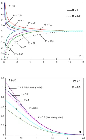
Results plotted on fig. 2.6 and 2.7 have been obtained from the differential method (§.2.2.1) and for a water flow (Pr = 7). The parameter Rt means T*p1 / T*p2. In these two cases, the steady state
is reached at a dimensionless time t+ close to 4,36 (see also § 2.2.4.6
for transient state duration). Fig.2.8 shows the evolution of the instantaneous dimensionless coefficient h+ in the same thermal conditions and for several values of Pr. It can be seen that highest Pr correspond to longest time durations.
0 0,2 0,4 0,6 0,8 1
0 0,5 1 1,5 2 2,5 3
ηηηη T* (ηηηη,t+)
t+ > 4.36 (final steady state)
t+ = 1
t+ = 0.5
Pr = 7
t+ = 0 (initial steady state)
t+ = 0.25
t+ = 2
Rt = 0.5
Figure 2.6. Transient temperature profiles for a negative step change in the plate temperature.
0 0.4 0.8 1.2 1.6 2
0 0.5 1 1.5 2 2.5 3
ηηηη T*
(ηηηη,t+
) Pr = 7
t+ > 4.36 (final steady state)
t+ = 1
t+ = 0.5
t+ = 0 (initial steady state)
t+ = 0.25
t+ = 2
Rt = 2
-4 -3 -2 -1 0 1 2 3 4 5 6
0 2 4 6 8 10 12
h+ (t+)
Pr = 0.71
Rt = 2
Rt = 0.5
Pr = 100 Pr = 20
Pr = 7
t+
Pr = 0.71
Pr = 100 Pr = 20
Pr = 7
0 0.2 0.4 0.6 0.8 1 1.2
0 0.5 1 1.5 2 2.5
ηηηη
G (ηηηη,t+
) Pr = 7
Rf = 0.5
t+ > 7.3 (final steady state)
t+ = 3.65
t+ = 1
t+ = 0 (initial steady state)
t+ = 0.5
Figure 2.9. Transient temperature profiles for a negative step change in the plate heat flux.
Uniform Heat Flux Steps
a)- Step from a zero state, followed by relaxation [8]
In order to discuss the behaviour of the boundary layer thickness in the general case, it is necessary to make a short description of the heating process from an isothermal state. In that case, we can attend the birth of a thermal boundary layer, which thickness δT grows
from zero to its stationary value (an illustration is given § 2.2.4.3, fig. 2.13).
Now, from the stationary state, heating is cut suddenly: the thermal boundary layer changes in a very different way: it does not collapse, it uniformly vanishes, without any variation in its thickness.
b)- Change from a heating steady state to another one [8] [11] [12] [13]
Consider now heating or cooling phases from a first heating steady state. We know that, in steady state, δT does not depend on
the wall heat flux. So we are allowed to assume that δT remains
constant during a heating phase. Indeed, this assumption has no interest with the differential method, but is very essential and useful in the Karman - Pohlhausen method, in which δT is a fundamental
parameter.
Some results are presented below. The curves plotted on fig. 2.9 and 2.10 were obtained from the differential method. The parameter G is the dimensionless temperature corresponding to an imposed wall heat flux Φ, and Rf = Φfinal / Φinitial. They show that the thermal
boundary layer thickness does not change during the transient state, and that the duration of this transient is longer than in the case of a
temperature step (t+ around 7.3 instead of 4.36, § 2.2.4.1; see also § 2.2.4.6).
0 0.4 0.8 1.2 1.6 2 2.4
0 0.5 1 1.5 2 2.5
ηηηη G (ηηηη,t+
) Pr = 7
t+ =3.65
Rf = 2
t+ > 7.3 (final steady state)
t+ = 1
t+ = 0.5
t+ = 0 (initial steady state)
Figure 2.10. Transient temperature profiles for a positive step change in the plate heat flux.
Figures 2.11 and 2.12 show results obtained from the integral method, with an air flow. Two step changes arise at times t = 0 and t = 0.3 s. It can be observed that the wall temperatures at different abcissas x admit a common envelope corresponding to the final steady state, and that the response is slower as x increases.
As for instantaneous Nusselt numbers, they decrease from infinity after each step.
0 2 4 6 8 10 12 14 16 18 20
0 0.1 0.2 0.3 0.4 0.5 0.6 0.7 0.8 0.9 1
Time (s) 1 cm
20 cm
15 cm
10 cm
5 cm
25 cm
θθθθ
p
(
K
)
Figure 2.11. Wall temperatures in the case of heat flux steps, from 10 to 100 W/m².
0 20 40 60 80 100 120 140 160 180 200
0 0.1 0.2 0.3 0.4 0.5 0.6 0.7 0.8 0.9 1
Time (s)
N
u
1 cm 10 cm 5 cm
25 cm
100
10
t 0
φφφφ(w/m²)
t1
1 cm 15 cm 20 cm
25 cm
Spatially Varying Heat Flux Steps [14] [15]
An extension of the KP model has been performed, in which arbitrary flux densities are applied along the wall.
Figure 2.13. Sinusoidal wall heat flux ϕϕϕϕ(x) step (from ϕϕϕϕ = 0).
First, fig. 2.13 shows the thermal response to a heat flux step, when the spatial distribution of ϕ(x) is sinusoidal. The diagram right is of special interest, as it shows the creation of a boundary layer, and the variation in time of its thickness, from zero to the steady state value (§ 2.2.4.2,a).
The following figures correspond to step changes from / to three different spatial heat flux distributions, denoted as ϕ1, ϕ2, ϕ3 (fig.
2.14), including a heating process from uniform temperature, and a sudden change from cooling to heating (fig. 2.19). Specially, pay attention to fig. 2.21, corresponding to this last case. It shows a kind of propagation wave of the heat transfer coefficient, and the displacement of the point where the wall temperature equals zero, corresponding to h = ∞.
0 50 100 150 200 250
0 0.03 0.06 0.09 0.12 0.15
ABSCISSA (m)
ϕ
(x
)
F
L
U
X
F
U
N
C
T
IO
N
S
(
W
/m
²)
ϕ2 = 50 exp(10x)
ϕ3 = 10 exp(10x)
ϕ1 = 150 exp(-10x)
Figure 2.14. Choice of arbitrary flux densities.
0 1 2 3 4 5 6 7 8 9 10
0 0.03 0.06 0.09 0.12 0.15
ABSCISSA (m)
W
A
L
L
T
E
M
P
E
R
A
T
U
R
EΘΘΘΘ
w
(K
)
t = 0.01s 0.03
0.07
0.12 0.18
0.27 0.54
Figure 2.15. Unsteady wall temperature in heating process [0→→ϕϕϕϕ→→1(x)].
0 5 10 15 20 25
0 0.03 0.06 0.09 0.12 0.15
ABSCISSA (m)
W
A
L
L
T
E
M
P
E
R
A
T
U
R
EΘΘΘΘ
w
(
K
)
t = 0s
0.54 0.04
0.12
0.20 0.30
0.40
Figure 2.16. Wall temperature evolution in the case [ϕϕϕϕ2(x) →→ϕϕϕϕ→→3(x)].
0 5 10 15 20 25
0 0.03 0.06 0.09 0.12 0.15
ABSCISSA (m)
W
A
L
L
T
E
M
P
E
R
A
T
U
R
E
ΘΘΘΘ
w
(K
)
t = 0s
0.54
0.12
0.20 0.04 0.02
0.08 0.06
Figure 2.17. Wall temperature evolution in the case [ϕϕϕϕ2(x) →→ϕϕϕϕ→→ 1(x)].
0 2 4 6 8 10
0 0.03 0.06 0.09 0.12 0.15
ABSCISSA (m)
W
A
L
L
T
E
M
P
E
R
A
T
U
R
E
ΘΘΘΘ
w
(
K
) t = 0s
0.02
0.06
0.28 0.20 0.14 0.10
Figure 2.18. Wall temperature evolution in fully cooling phase [ϕϕϕϕ1(x) →→→→✁
].
-5 -2.5 0 2.5 5
0 0.03 0.06 0.09 0.12 0.15
ABSCISSA (m)
W
A
L
L
T
E
M
P
E
R
A
T
U
R
EΘΘΘΘ
w
(
K
)
t = 0s 0.04
0.10 0.15
0.20 0.25
0.30 0.40 0.54
-4 -2 0 2 4
0 0.2 0.4 0.6
TIME (s)
Q
T
H
E
R
M
A
L
F
L
O
W
R
A
T
E
(
W
/m
)
X = 0.02m 0.05
0.10 0.15
Figure 2.20. Thermal flow rate as a function of time for different abscissa (case [- ϕϕϕϕ3→→ϕϕϕϕ→→ 3]).
-200 -100 0 100 200
0 0.03 0.06 0.09 0.12 0.15
ABSCISSA (m)
h
C
O
E
F
F
IC
IE
N
T
(
W
/m²
.K
)
t=0s
0.04 0.04
0.10
0.10 0.15
0.15 0.20
0.25
0.54
Figure 2.21. Heat transfer coefficient for different times (case [- (3((3]).
Uniform Periodic Heat Flux [16]
A situation of practical interest consists in periodic boundary conditions, uniform periodic heat flux as example. A comparison between three different signal shapes (in time) is reported on fig. 2.22. As it can be seen, successive sinusoidal signals give a higher average wall temperature than triangular ones.
0 5 10 15 20 25 30
0 0,05 0,1 0,15 0,2 0,25 0,3
Temps (s)
Flux triangulaire Flux sinusoïdal
Flux constant =100 W/m²
Tp -Ti (Moyenne K)
Figure 2.22. Average temperatures corresponding to different shapes of periodic flux Air flow. Period T = 0.008 s.
Dimensioned and Dimensionless Results [12] [13] [17] [20]
Regarding experimental or numerical results in convective heat transfer, a very important issue consists in the best way to express them: by the mean of dimensioned or dimensionless data? Of course, dimensionless numbers seem to be more convenient, as they
combine several physical parameters. But they can drive to wrong interpretations, because the appearances that we are able to see in the results can be very different according as they are dimensioned or not. Moreover, in a practical way, engineers are interested only by dimensioned data. Two examples are given below (see also § 2.2.4.2).
In the first case, heat flux density suddenly decreases. The Nusselt number and the heat transfer coefficient h (in an air flow) are plotted versus time: it can be easily observed that their trends appear very different (fig. 2.23, 2.24).
0 20 40 60 80 100 120 140 160 180 200
0 0.1 0.2 0.3 0.4 0.5 0.6 0.7 0.8 0.9 1
Tim e (s) N u
20 cm 25 cm 100
10
t 0
φφφφ(w /m²)
1 cm
10
10
5
1 cm
20 15
25
5 cm
t1
15 cm
Figure 2.23. Sudden cooling: Nusselt number as a function of dimensionless time.
0 5 10 15 20 25 30
0 0.1 0.2 0.3 0.4 0.5 0.6 0.7 0.8 0.9 1
Time (s)
h
c
(
W
.m
-2.K -1)
1 cm
20 cm 15 cm 10 cm 5 cm
25 cm 1 cm
10 cm 5 cm
Figure 2.24 . Sudden cooling: heat transfer coefficient, at different locations x.
In the second case (fig. 2.25, 2.26) a temperature step is imposed on the wall, in a water flow (U∞= 0.5 m/s). A unique curve describes the evolution of the dimensionless wall heat flux (T*)’ as a function of dimensionless time t+, but h versus dimensioned t does not obey to the same rule, and crossings in the curves appear, that cannot be guessed from the dimensionless plotting.
0,5 1 1,5 2 2,5 3
0 1 2 3 4 5 6
t+
-T
*'
(0
,t
+ )
0 500 1000 1500 2000
0 2 4 6 8
time (s)
h
(
W
/m
2 K
)
x = 0.1m x = 0.2m x = 0.5m x = 1m
Figure 2.26. Instantaneous convective heat transfer coefficient at different abscissa.
Transient State Duration [5] [12] [18] [19]
Another fundamental and practical problem consists in characterising the “response speed” of a system. This can be done in several ways, for example:
1- Time constant τ deduced from an exponential fitting of the temperature response, as shown below (fig. 2.27) in a Blasius air flow (U∞ = 1 m/s), with a heat flux step [18].
Figure 2.27. Time constant in seconds (air flow, velocity = 1 m/s).
2- Transient duration defined as the time when the difference between instantaneous and steady state heat transfer coefficients become less than 1% [19] [12].
An example is given on Table 1 for a wall temperature step on a wedge or in a velocity gradient flow (§ 2.2.1). It shows that the transient duration d (expressed in seconds) for the wall heat flux increases with x, except near m = 1 where it becomes independent of x. Obviously, it increases also with Pr.
Once more, this offers the opportunity to pay attention to dimensioned compared to dimensionless presentation of numerical results. Dimensionless results show a transient duration increasing as m decreases [5]. On the contrary, it appears on Table 1 that the real (dimensioned) duration has a minimum for m close to zero.
Complementary data about transient durations can be found in § 2.2.4.1.
Table 1. Flow over a wedge: dimensioned transient duration d (in seconds).
Pr m ββββππππ/2 U∞∞∞∞ (m/s) in x1 = 0.166 m
d (s) in x1 U∞∞∞∞ (m/s) in x2 = 0.5 m
d (s) in x2 U∞∞∞∞ (m/s) in x3 = 0.8 m
d (s) in x3
-0,0476 -π/20 0,545 0,647 0,517 2,053 0,505 3,359
0 0 0,500 0,572 0,500 1,724 0,500 2,758
0,111 π/10 0,410 0,663 0,463 1,766 0,488 2,682
0,333 π/4 0,275 0,934 0,397 1,949 0,464 2,666
0,71
1 π/2 0,083 2,917 0,250 2,917 0,400 2,917
-0,0476 -π/20 0,545 1,474 0,517 4,679 0,505 7,655
0 0 0,500 1,304 0,500 3,929 0,500 6,286
0,111 π/10 0,410 1,510 0,463 4,026 0,488 6,113
0,333 π/4 0,275 2,129 0,397 4,441 0,464 6,077
7
1 π/2 0,083 6,649 0,250 6,649 0,400 6,649
-0,0476 -π/20 0,545 3,839 0,517 12,187 0,505 19,940
0 0 0,500 3,398 0,500 10,234 0,500 16,374
0,111 π/10 0,410 3,934 0,463 10,485 0,488 15,924
0,333 π/4 0,275 5,545 0,397 11,569 0,464 15,828
100
1 π/2 0,083 17,319 0,250 17,319 0,400 17,319
Finite Thickness Plate
The case of a finite thickness plate is of better practical interest, but is also more difficult to solve by the mean of half – analytical methods. Indeed, the differential method is inadequate to describe conduction -–convection coupled problems. Integral methods can be extended to such situations, but does not seem more suitable than purely numerical methods.
Backward Face: Temperature Step [21] [22]
phase, due to the boundary condition on the upward face of the plate.
Figure 2.28. Temperature profiles in the PVC wall (y/E ) and in the air (y/δδδδ), x = 15 cm.
Upward Face: Heat Flux Step [23]
Consider now a plate isolated on its backward face, and submitted to a heat flux step on the flow side face (upward face): this example corresponds to an experimental set-up used for the measurement of the heat transfer coefficient (§ 5). The same integral method has been recently applied to the determination of the temperature field (fig. 2.29).
0 0.05 0.1 0.15 0.2 0.25 0.3 0.35 0.4 0.45
-0.007 -0.005 -0.003 -0.001 0.001 0.003 0.005
Y(m) dans la plaque Y(m) dans le fluide Tp-Ti
x = 0.01 x = 0.02 x = 0.03 x = 0.04
x = 0.05 temps = 0.035 s
Profils de température pour t = 0.035 s
0 0.5 1 1.5 2 2.5 3 3.5 4
-0.007 -0.005 -0.003 -0.001 0.001 0.003 0.005
Y(m) dans la plaque Y(m) dans le fluide Tp-Ti
x = 0.01
x = 0.02
x = 0.03
x = 0.04 x = 0.05 temps = 0.28 s
Profils de température pour t = 0.28 s
Figure 2.29 . Heat flux steps on the upward face of the plate temperature profiles in the wall and in the fluid at different times.
0 0.5 1 1.5 2 2.5 3 3.5 4 4.5 5
-0.007 -0.005 -0.003 -0.001 0.001 0.003 0.005
Y(m) dans la plaque Y(m) dans le fluide Tp-Ti
x = 0.01 x = 0.02 x = 0.03
x = 0.04 x = 0.05 temps = 0.42 s
Profils de température pour t = 0.42 s
0 1 2 3 4 5 6
-0.007 -0.005 -0.003 -0.001 0.001 0.003 0.005
Y(m) dans la plaque Y(m) dans le fluide Tp-Ti
x = 0.01 x = 0.02 x = 0.03
x = 0.04 x = 0.05 temps = 0.56 s
Profils de température pour t = 0.56 s
0 1 2 3 4 5 6 7
-0.007 -0.005 -0.003 -0.001 0.001 0.003 0.005
Y(m) dans la plaque Y(m) dans le fluide Tp-Ti
x = 0.01
x = 0.02
x = 0.03 x = 0.04
x = 0.05 temps = 0.63 s
Profils de température pour t = 0.63 s
0 1 2 3 4 5 6 7
-0.007 -0.005 -0.003 -0.001 0.001 0.003 0.005
Y(m) dans la plaque Y(m) dans le fluide Tp-Ti
x = 0.01 x = 0.02
x = 0.03 x = 0.04
x = 0.05 temps = 0.77 s
Profils de température pour t = 0.77 s
Figure 2.29 .(Continued).
Impinging Jets
backward face. Numerical solution is obtained by the mean of an integral approach, using 4 – degree polynomials. A panel of results can be found in ref. [24].
Natural Convection
Introduction
Among the three types of convective transfers, forced convection is often used because of its efficiency. A contrario, natural convection has the advantage to be free in terms of energy expense but generates low heat transfer coefficient. Thus it will be interesting to improve free convection heat transfer, by the mean of time-dependent boundary conditions.
Laminar free convection problem on a vertical wall has been plentifully investigated considering constant wall heat flux or wall temperature. But it appears in literature that the dynamic behaviour of free convection flows is poorly documented.
Some recent investigations carried out with various time-dependent boundary conditions are presented below. They deal with free convection over a vertical plate (fig. 3.1) and were performed by the mean of extended differential or integral methods.
Equations to be solved are the same as in § 2.2.1 except the momentum equation that becomes:
∂U/∂T + U ∂U/∂x + V ∂U/∂y = gβ(T - T∞) + ν∂2U/∂y2
Figure. 3.1. Velocity layer and coordinates system.
Differential Method
An extension of the method described by Cebeci [2] has been proposed, which involves a generalisation of the differential method, and the use of Keller-box method to solve the equations.
The results are quite similar to those obtained with the integral method, except far from the wall where the differential method gives higher boundary layer thickness [25 to 28].
In the case of periodical wall heat flux, it was found that the thermal boundary layer thickness does not vary and that for low period rates, when the steady state is reached, heat transfer coefficient h gets its optimal value.
Integral Method
Using the Karman-Pohlhausen integral method [1, 29], physically polynomial profiles of fourth order are assumed for flow velocity and temperature across the corresponding hydrodynamic
and thermal boundary layers. The method of analysis assumes that the velocity and temperature distributions have temporal similarity, meaning that the ratio Ω between the thermal thickness δT and the dynamical thickness δ depends only upon the Prandtl number during the transient [30, 31, 32]:
) t , x ( (Pr) ) t , x ( T δ
δ =Ω
Thus, combining this relation with Fourier’s law and adequate boundary conditions leads to the following U-velocity and Θ -temperature polynomial distributions depending mainly upon the δ dynamical parameter [33]:
[
η η η η]
ν λ
δ ϕ
β Ω − + − +
= 3 4 3 2
3 3 12 w g U ; ) ( T
T w T 2 T 2 T 1
2
3
4+ − +
− Ω = − =
Θ ∞ ϕ λδ η η η
where η = y/δ ≤ 1, ηT = y/δT ≤ 1. Parameters β, λ, ν, ϕw are
respectively the volumetric coefficient of thermal expansion, the thermal conductivity of the fluid, the kinematic viscosity, and the wall heat flux density.
The integral forms of the boundary-layer momentum and energy conservation equations become then:
∫ ∫ ∂ Θ ∂ − = Θ ∂ ∂ + Θ ∂ ∂ ∫ ∫ ∫ ∂ ∂ − Θ ∂ ∂ = ∂ ∂ + ∂ ∂ Ω Ω = Ω = δ δ
δ δ δ
ν ν β 0 0 0 0 0 0 0 2 y y y Pr Udy x dy t y U dy x g dy U x Udy t
The analytical resolution of the system under the assumption
∂/∂t = 0 leads to the knowledge of the boundary layer ratio Ω and on the other hand gives the steady evolution of the asymptotical -solution.
Thus, introducing the parameter K = ln(Pr), the evolution of the ratio Ω(Pr) is found to be suitable whatever Pr > 0.6 and satisfactorily approached with the following relation :
901 0 1961 0 10 282 4 10 227 4 0 1 576
1. -4K4− . -3K3+ . 2K2− . K+ .
=
Ω −
The asymptotical limit of the dynamical boundary layer thickness is analytically expressed as:
5 1 2 5 9 432 − Ω Ω = ∞
→ ( )x
g ) t , x ( w ϕ β ν λ δ
Considering the transient regime and using the assumption Ω = cst, the resolution leads to the combined resulting governing equation of the free convection problem :
0 Pr 3 10 5 9 2 36 56 9 14 5 3 12 2 7 5 2 4 5 4 3 2 w = Ω + − Ω − ∂ ∂ Ω − Ω + Ω − Ω + Ω + ∂
∂ δ δ ν
νλ βϕ δ δ x g t
with the following boundary conditions:
0 ) , 0 ( ) 0 ,
(xt= =
δ
x= t =δ
. Results
Eckert’s Theory Revisited [30]
A preliminary issue dealt with the velocity and thermal boundary layers.
First consider that, basically, two different definitions of a boundary layer thickness are commonly used, as for forced, mixed or natural convection:
a)- A standard definition in agreement with the asymptotic structure of a boundary layer: at a distance from the wall equal to the layer thickness, the variation of the considered parameter (velocity, temperature gap) reaches 99% of its total value.
b)- A mathematical definition linked to the Karman – Pohlhausen method: in this theory, the velocity and temperature fields are described by two polynomials, and δ (or δT) are the
distances from the wall where these polynomials are equal to zero. Anyway, for a long time, Eckert’s theory was accepted. It assumed that, in steady natural convection along a vertical flat plate,
δ = δT. This assumption was very useful as it gave a simple way to
obtain the h coefficient, but in fact, had no real physical support and it appeared necessary to check it. A study driven by the mean of the integral method [30] concluded that it is acceptable for the computation of h, but is not adequate for the description of the dynamical field. It was shown that δ / δT depends on Pr, and a
relation δ / δT = Ω (Pr) was proposed for a large range of Prandtl
numbers.
Evolution of Boundary Layers [33]
In natural convection, dynamical and thermal fields are linked, so that transient phenomena are of special interest. A panel of results is presented below; all of them have been got from the integral method.
On fig. 3.2, dynamical boundary layer thickness is plotted at different times, in the case of a wall heat flux ϕw = 100 W/m2 in
initially quiescent water (Pr = 7). As predicted by other authors, the transients in free convection are found to start as a one-dimensional conduction process, to be terminated by the arrival of the leading edge effect. This is the reason why the viscous layer profiles present a flat vertical shape in the early transient. Fig.3.3. is a plot of velocity at the chosen elevation x = 0.10 m within the viscous boundary layer where the velocity distributions are shown to increase in time to reach a steady profile in close agreement with the commonly presented shape in literature.
Figure 3.2. Transient behaviour of the velocity boundary layer.
Figure 3.3. Transient velocity profiles at the x = 0.1 m abscissa.
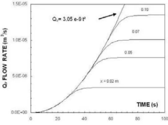
Figure 3.4. Volumetric flow rate versus time.
To complete this hydrodynamic analysis, variations of the volumetric flow rate with position and time have been investigated. Thus the integral formulation indicates that the flow rate grows downstream as x0.8. It is worth mentioning from fig.3.4 that whatever the x-position, before reaching its asymptotical value, the transient volumetric flow rate evolves in time as t2.
Dimensioned Versus Dimensionless Results
As it was mentioned in the second part (forced convection, § 2.2.4.5), dimensionless laws can suggest trends very different from dimensional ones. Another illustration applied to natural convection can be found in [34]. It concerns the time-dependence of the heat transfer coefficient for a panel of usual fluids.
Free Convection Around Cylinders Mounted on a Plate [35, 36]
Flow visualisation is a very efficient experimental meaning to get information on the dynamical behaviour of fluid flows. Two kinds of techniques were employed to get streamlines in the meridian section of the flow. The first one is based on an electrolytic precipitation method leading to the generation of white smoke composed of metallic salt used as a tracer material. In the experiments, electrolysis of water is made by applying a voltage between a tin wire considered as an anode, and a copper plate inside the water tank as a cathode. For the second one, the fluid is seeded with suspended fine rilsan particles (75 < diameter < 150 µm, ρ = 1.06 g/cm3) illuminated by a laser sheet (2 W argon laser) from which instantaneous integrated streamlines can be drawn.
The first study describes experiments on flow visualization and local convective heat transfer of three-dimensional cylinders embedded in a transient natural boundary layer under uniform wall heat flux condition (fig. 3.5 and 3.6).
Figure. 3.5. Schematic of the experimental model.
Figure 3.6. Angular positions of a square cylinder.
Figure 3.7. Heat transfer performance of a square cylinder compared with the smooth plate.
Especially, emphasis is put on the influence of the angular positions of the cylinder around a given axis and on its square or circular geometry on both local thermal measurements and flow patterns. For example, it is shown that for the square cylinder, a 60° position induces a singular behaviour by reducing the convective heat transfer coefficient (fig.3.7); this singularity is confirmed with visualisations of the separation region.
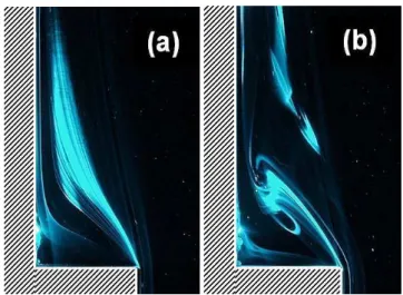
To have an idea of the near wake shape, in fig.3.8 are presented examples in the symmetrical (P,Y,Z) plane. Details are seen from metallic salts emitted from both downstream and upstream the obstacle. One can see the separation area downstream and the development of vortical structures just behind the bluff body.
Figure 3.8. Details of the near wake for αααα = 0 at two times t = 120 s (a) and t = 170 s (b).
Free Convection Along Large – Scale Roughness Plate [37]
Moreover, transient natural convection on a vertical ribbed wall has been studied experimentally with a wall – boundary condition of uniform heat flux. This situation is of importance to both fundamental scientific research in understanding the interaction between large-scale flow features and local heat transfer, and practical interest in many industrial applications such as electronic equipment or climate control within building interiors where passive heating and cooling techniques are employed.
I II III
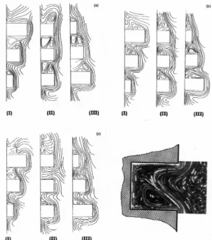
Figure 3.9. Streakline patterns visualised with an electrolytical precipitation method (t = 300s).
Figure 3.10. Instantaneous streamlines: (a) t = 57 s; (b) t = 112 s; (c) t = 610 s. Right below: detail of the rotational flow in the lower cavity, configuration (II), t = 112 s.
Mixed Convection
Introduction
Unsteady mixed convection problems can occur in various thermal systems, either occasionally or when the boundary conditions are normally changing with time. The first kind of situations can be met in starting processes, or accidental transients, regarding for example security in power plants and electric transformers. In the second one, interest is stimulated by the needs of regulation of heat transfer equipment, as hot water heating systems in buildings.
Publications reported here deal with computational studies on water flows in vertical pipes, especially when steps of temperature or flow rate are imposed at the entrance (fig. 4.1). Two methods have been employed, either by using the classical parameters (§ 4.2) or by introducing the vorticity function (§ 4.3). The first formulation is more usual, but the second one suits better for describing reverse flows, and does not need any assumption on the pressure term.
Figure 4.1. Schematic of the mixed convection model..
Direct Solution Method [38, 39]
The physical system under consideration is a vertical pipe of radius R. The z axis is chosen to follow the flow direction (upward or downward). The fluid is considered to be newtonian with constant dynamic viscosity, conductivity, specific heat capacity and expansion coefficient. Density variations are assumed to be negligible except in the buoyancy term of the vertical momentum equation (Boussinesq approximation). So the problem can be formulated by the governing equations, expressed by the mean of cylindrical coordinates: continuity, axial-momentum and energy.
0 r V r V z
U =
∂ ∂ + + ∂ ∂
∂ ∂ + ∂ ∂ ν + − β ε + ∂ ∂ ρ − = ∂ ∂ + ∂ ∂ + ∂ ∂
2 2
w e *
r U r U r 1 ) T T ( g z p 1 r U V z U U t U
∂ ∂ + ∂ ∂ α = ∂ ∂ + ∂ ∂ + ∂ ∂
2 2
r T r T r 1 r T V z T U t T
with p*=p−ρgz ; upward flow : ε = + 1 ; downward flow : ε = - 1 The physical problem is characterised by the following initial and boundary conditions:
- thin pipe wall
- on the outer surface of the pipe: averaged free convection heat transfer, so that the wall heat flux is:
) T T (
h w
w = − ∞
ϕ
- on the inner surface (r = R):
U = V = 0
- on the axis (r = 0):
0 r T r
U =
- at the entrance (z = 0) : fully developed velocity profile
o
U and injection temperature Te:
- t < 0: flow rate qo ; Reynolds Reo, temperature T0
-
t
≥
0
: flow rate qe = qo + ∆qe (∆qe > 0 or < 0), i.e. Re∞= Reo + ∆Re
and / or temperature Te = T0 + ∆Te (∆Te > 0 or < 0)
- at the exit (z = L): ∂U / ∂z = 0
Equations were solved by a finite-difference, fully implicit procedure. The pressure gradient was written as the sum of a steady term and of a time – dependent term in relation with the flow rate conservation [39].
Vorticity Method [40, 41]
The situation considered is a laminar flow upward through a vertical pipe, that is imposed by a heat transfer coefficient on the outer surface of the pipe. Flow entering the pipe is solicited by a temperature step. In this part, governing equations are formulated in terms of the stream function Ψ and the vorticity Ω, with the following dimensionless quantities:
2 ; ; ; ; ; ; R V V R R t V t T T T T T V V V V U U R z z R r r d d d a e a d d ψ ψ = Ω = Ω = − − = = = = = + + + + + + + + ; 1 1 + + + + + + + + ∂ ∂ = ∂ ∂ − = r r V ; z r
U ψ ψ +
+ + + + ∂ ∂ − ∂ ∂ = Ω r V z U
The non-dimensional equations in terms of these variables and temperature are :
2 2 1 1 + + + + + + + + ∂ ∂ + ∂ ∂ ∂ ∂ = Ω − z r r r r ψ ψ
( ) ( )
+ + + + + + + + + + + + + + + + + ∂ ∂ + ∂ Ω ∂ + ∂ Ω ∂ ∂ ∂ = ∂ Ω ∂ + ∂ Ω ∂ + ∂ Ω ∂ r T Ri z r r r r Re r U z V t 2 2 1 1(
) ( )
∂ ∂ + ∂ ∂ ∂ ∂ = ∂ ∂ + ∂ ∂ + ∂ ∂ + + + + + + + + + + + + + + + + + 2 2 1 1 1 z T r T r r r Pe z T V r T U r r t TThe initial and boundary conditions are as follows:
1 1
0 1 0
0 ≤ ≤ ≤ ≤ =
< + + +
+ , z , r : T
t (uniform temperature)
t+≥ 0 ,
+ + + + + + +
+ − Ω = = +∆
− =
= : r r ; r ;T T
z 4 1
2 1 2 1 0 2 ψ
where + ∆ +
− ∆ =
∆ ( T
T T T T a e e
> 0 or < 0)
0 0
0 = Ω =
∂ ∂ = ∂ ∂ = ++ ++ + + ; r r T : r ψ + + + + + =− ∂ ∂ =
= * w
w T Bi r T ; :
r 1 ψ 0
where
f a
* h R
Bi
λ
= (generalised Biot number)
The foregoing equations were solved by a finite – difference procedure, with an explicit numerical scheme [41].
Applications
Temperature Steps at the Entrance [41]
As an application of the vorticity method, the following conditions were selected: upward water flow, pipe of diameter 20 mm, bulk velocity = 0.045 m/s. On the external surface, authors assumed a constant mean coefficient ha = 5 W/m2.K, with ambient
air at Ta = 20 °C.
Regarding the case where ∆Tinlet = + 10 °C, velocity and
temperature profiles have been plotted on fig. 4.2, at a distance from the entrance z = 200 mm. A short time after the perturbation, under buoyancy effect the fluid velocity increases in the central part and decreases near the wall, with an invariant point at r+ ≈ 0.66; the
distortion is maximal at about 11 s, and can lead to reverse flow. In the case of a negative step (∆T = -10 °C, fig. 4.3) the velocity profile shows another kind of distortion, with a fluid velocity increasing first near the wall and decreasing in the central part. The perturbation reaches its maximum value sooner (at t ≈ 9 s) and is stronger with increasing distance from the entrance.
-0.5 0 0.5 1 1.5 2 2.5 3
0 0.2 0.4 0.6 0.8 1
r+
V
+
t = 0 s t = 2 s t = 4 s t = 7 s t = 11 s t = 26 s
0.95 1 1.05 1.1 1.15 1.2 1.25 1.3 1.35 1.4
0 0.2 0.4 0.6 0.8 1
r+
T
+
t = 0 s t = 2 s t = 4 s t = 7 s t = 11 s t = 26 s
0 0.2 0.4 0.6 0.8 1 1.2 1.4 1.6 1.8 2
0 0.2 0.4 0.6 0.8 1
r+
V
+
t = 0 s t = 2 s t = 4 s t = 9 s t = 11 s t = 20 s
0 0.2 0.4 0.6 0.8 1 1.2 1.4 1.6 1.8 2
0 0.2 0.4 0.6 0.8 1
r+
V
+
t = 0 s t = 2 s t = 4 s t = 9 s t = 11 s t = 20 s
Figure 4.3. Velocity profiles for z = 200 mm (left) and z = 600 mm (right), ∆∆∆∆T = - 10 °C.
Flow Rate Steps [39, 42]
Using direct solution method, other studies have dealt with flow rate steps, positive or negative (fig. 4.4 and 4.5). In such circumstances, perturbations in the velocity field are rather progressive with an increase of flow rate, but more complex in the case of negative steps. Computations show also that the response is slower with negative steps (fig. 4.6) as the contrary was observed with temperature steps. Moreover, the buoyancy ratio RiRe has a strong influence on the wall heat transfer [42].
0 2 4 6
0 2 4 6 8 10
Radius (mm)
V
e
lo
c
it
y
(c
m
/s
)
t = 0 s t = 20 s t = 23 s t = 27 s t = 50 s
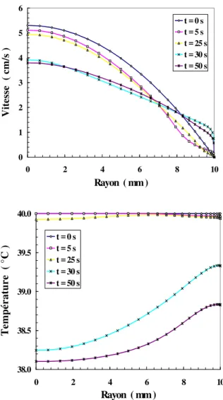
Figure 4.4. Velocity and temperature profiles for different times at z = 300 mm qv=+5l/h ; Te = 40 °C ; Reo = 530 ; Re∞∞∞∞ = 620 ; Gr = 3.105 ; RiRe∞∞∞∞ = 484.
40.0 40.5 41.0 41.5 42.0
0 2 4 6 8 10
Radius (mm)
T
e
m
p
e
ra
tu
re
(°
C
)
t = 0 s t = 20 s t = 23 s t = 27 s t = 50 s
Figure 4.4. (Continued).
0 2 4 6
0 2 4 6 8 10
Radius (mm)
V
e
lo
c
it
y
(c
m
/s
)
t = 0 s t = 25 s t = 27 s t = 30 s t = 50 s
40.0 40.5 41.0 41.5 42.0
0 2 4 6 8 10
Radius (mm)
T
e
m
p
e
ra
tu
re
(°
C
)
t = 0 s t = 25 s t = 27 s t = 30 s t = 50 s
10 15 20 25 30 35
-1 2 -1 0 -8 -6 -4 -2 0 2 4 6 8 1 0 1 2
F low ra te s tep (l/h)
T
im
e
c
o
n
s
ta
n
t
(
s
)
D qv > 0 D qv < 0
Figure 4.6. Time constant evolution for positive and negative flow rate steps at z = 400 mm ; Re = 530; T0 = 40 °C.
Combined Temperature and Flow Rate Steps
Unfortunately, combined temperature and flow rate steps have not been widely investigated, despite of their special interest as they can lead to amplified or smoothed effects, depending on their sign and amplitude. Examples plotted on fig. 4.7 to 4.9 come from ref. [43] and show in a special case that the friction factor along the wall is more regular when the two steps are positive.
0 1 2 3 4 5 6 7
0 2 4 6 8 10
Rayon ( mm )
V
it
es
se
(
cm
/s
)
t = 0 s t = 20 s t = 24 s t = 30 s t = 50 s
40.0 40.5 41.0 41.5 42.0
0 2 4 6 8 10
Rayon ( mm )
T
em
p
ér
a
tu
re
(
°C
) t = 0 s
t = 20 s t = 24 s t = 30 s t = 50 s
Figure 4.7. Velocity and temperature profiles at z = 300 mm ; ∆∆∆∆qv = + 5.10 -3
m3
/h, ∆∆∆∆T = + 2 °C, qvo = 3.10-2 m3/h, Teo = 40 °C, ha = 10 W/m2.K.
0 1 2 3 4 5 6
0 2 4 6 8 10
Rayon ( mm )
V
it
es
se
(
cm
/s
)
t = 0 s t = 5 s t = 25 s t = 30 s t = 50 s
38.0 38.5 39.0 39.5 40.0
0 2 4 6 8 10
Rayon ( mm )
T
em
pé
ra
tur
e
(
°
C
)
t = 0 s t = 5 s t = 25 s t = 30 s t = 50 s
Figure 4.8. Same datas as on fig. 4.7. except ∆∆∆∆qv = - 5.10 -3
m3/h ;
∆∆∆∆T = - 2 °C.
0 1 2 3 4 5 6 7 8
5 10 15 20 25 30 35 40
z/R
Cf
*
1
0
-4
échelon positif échelon négatif
Flow Instabilities [44, 45]
Very interesting complementary informations on the structure of the flow are brought by streamlines and isotherms [44], as they specially permit to observe reverse flows and vortex that can occur during the transient (see examples on fig. 4.10 and 4.11). These structures are of practical interest because of their influence on friction and heat transfer at the wall, but also of fundamental importance, as they can be considered as signs of instability.
0 5 10
0 100 200 300 400 500 600 700 800
0 5 10
0 100 200 300 400 500 600 700 800
0 5 10
0 100 200 300 400 500 600 700 800
0 5 10
0 100 200 300 400 500 600 700 800
0 5 10
0 100 200 300 400 500 600 700 800
0 5 10
0 100 200 300 400 500 600 700 800
(a) (b) (c)
r (mm)
Ψ+ T+ Ψ+ T+ Ψ+ T+
z (mm)
Figure 4.10. Time development of streamlines and isotherms along the pipe for ∆∆∆∆T = +10 °C, (a): 5 s, (b): 15 s and (c): 25 s.
0 5 10
0 100 200 300 400 500 600 700 800
0 5 10
0 100 200 300 400 500 600 700 800
0 5 10
0 100 200 300 400 500 600 700 800
0 5 10
0 100 200 300 400 500 600 700 800
0 5 10
0 100 200 300 400 500 600 700 800
0 5 10
0 100 200 300 400 500 600 700 800
(a) r (mm) (b) (c)
z (mm)
Ψ+ T+ Ψ+ Ψ+
T+ T+
Figure 4.11. Time development of streamlines and isotherms along the pipe for ∆∆∆∆T = -10 °C, (a): 10 s, (b): 30 s and (c): 50 s.
Indeed, stability in transient states remain a widely open issue. As a starting point, two stability diagrams were proposed in the case of an upward flow, using similitude criteria Ri and Re (fig. 4.12). They show a stable zone (free of reverse flow or vortex) larger for negative than for positive temperature steps [45].
0.1 1 10 100 1000 10000
10 100 1000
Re Ri
Te=50 °C instable Te=40 °C instable Te=30 °C instable Te=50 °C stable Te=40 °C stable Te=30 °C stable
ZONE STABLE ZONE INSTABLE
0.1 1 10 100 1000 10000
10 100 1000
Re Ri
Te=50 °C instable Te=40 °C instable Te=30 °C instable Te=50 °C stable Te=40 °C stable Te=30 °C stable
ZONE STABLE ZONE INSTABLE
Figure 4.12. Stability diagrams Ri-Re for ∆∆∆∆Te > 0 (left) and ∆∆∆∆Te < 0 (right).
Mixed Convection Boundary Layers [46]
0 0.2 0.4 0.6 0.8 1 1.2
0 0.5 1 1.5 2 2.5 3 3.5
Y+
U
+
t+ = 0 .0 1
t+ = 3 1
t+ = 0 .5
-0 .2 0 0 .2 0 .4 0 .6 0 .8 1 1 .2
0 0.5 1 1.5 2 2 .5
Y+
U
+
t+ = 0 . 05
0 .1
0 .3 0. 6 1
3 5
Figure 4.13. Velocity profiles at different times t+ for a flow velocity step
∆∆∆∆U+ Pr = 1; E(ρρρρ Cp)wall /L(ρρρρ Cp)fluid = 5; left: aiding flow, RiRe = + 50, ∆∆∆∆U+ = -
0.4; right: opposing flow, RiRe = - 50, ∆∆∆∆U+ = + 0.4.
Measurement of the Heat Transfer Coefficient [18] [47 To 50]
A major practical application of transient convection deals with the measurement of heat transfer coefficients by pulsed photothermal radiometry.
The method consists of analysing the transient temperature on the front face of a wall, after a sudden deposit of luminous energy, and is generally used for non-destructive testing operations as well as measurement of thermophysical properties. But it was also proposed to consider pulsed photothermal radiometry as a tool for the measurement of convective heat transfer coefficient on the front side of the sample [47]. A scheme of the experimental device is presented on fig. 5.1.
Echantillon
Résistance chauffante Isolant
Détecteur Miroir Plan
Modulateur mécanique Miroir Concave
Enceinte de Protection Lampesflash
Ventilateur
Diffuseur d'Air
Air
Générateur de fréquence Préampli.
Ampli à détection synchrone.
Carte d'acquisition + Ordinateur
Table porte-échantillon Table porte-instruments
Figure 5.1. Experimental device.
A theoretical model was initially based on the assumption of a constant h coefficient during the transient used for the measurement. Compared to other experimental techniques as fluxmeters, the results gave rather good evaluations for h. An extension of this method was also described, allowing to simultaneous determination of the exchange coefficients on both sides of a thermally thin wall [48].
Indeed, assuming h = cst is not satisfactory if a precise measured value is required, and it becomes necessary to take into account that h = h(t) during the measurement process. So, results obtained from transient forced convection over a thin flat plate ([6, 11, 18], § 4.1) were used to introduce a variable coefficient h(t) in the theoretical model, as an exponential function of time [49, 50). This study leads to the conclusion that, in an air flow, h = cst in an adequate approximation with a dirac pulse. But in the case of finite duration pulses, this simplification is less and less valid as the duration increases (tables 5.1 and 5.2: lines 1 to 5 correspond to different values of air flow velocity, from 1.1 to 2.4 m/s), and a h(t) model gives more accurate values.
A second improvement will consist in considering the thickness and heat capacity of the plate, which modify h(t) compared to the case of a thin plate [20, 23].
Table 5.1. Convective heat coefficient in (W m-2 K-1) for dirac excitation.
Fluxmeter Model h cst
0 c
0 c h
h ∆
Model h(t) 0 c
0 c h
h ∆
1 37 35,2 -5% 40 +8%
2 50 46,5 -7% 49,5 -1%
3 62 67 +8% 63,2 +2%
4 74 77 +4% 71,8 -3%
Table 5.2. Convective coefficient in (W m-2
K-1
) for 5 s excitation.
Fluxmètre Model h cst 0 c
0 c h
h ∆
Model h(t) 0 c
0 c h
h ∆
1 37 49 +32% 42,3 +14%
2 50 65 +30% 56 +12%
3 62 70,6 +14% 67 +8%
4 74 80 +8% 80 +8%
Heat Exchangers Under Transient Conditions
Though it is based on an overall modelling, unsteady behaviour of heat exchangers can be considered as a special case of unsteady convection. It can occur in various conditions such as natural time-varying inlet temperatures or flow rates, start-ups, shut-downs, power surges, pump failures…. So an accurate knowledge of the thermal response of such systems during unsteady periods of operation is very important for effective controls, as well as for the understanding of the adverse effects which usually result in modified thermal performances or increased thermal stresses which will ultimately produce mechanical failure.
Assumptions and Modelling
![Figure 2.20. Thermal flow rate as a function of time for different abscissa (case [- ϕϕϕϕ3→→ →ϕϕϕϕ3])](https://thumb-eu.123doks.com/thumbv2/123dok_br/18974942.455029/6.892.104.415.134.340/figure-thermal-flow-function-different-abscissa-ϕϕϕϕ-ϕϕϕϕ.webp)