Regularizations: Different Prescriptions for Identical Situations
E. Gambin*, C. O. Lobo*, G. Dallabona**, and O. A. Battistel* * Dept. of Physics, Universidade Federal de Santa Maria
P.O. Box 5043, 97119-900, Santa Maria, RS, Brazil
Instituto de F´ısica Te´orica,Rua Pamplona, 145, 01405-900, S˜ao Paulo, SP, Brasil
Received on 10 December, 2004
We present a discussion where the choice of the regularization procedure and the routing for the internal lines momenta are put at the same level of arbitrariness in the analysis of Ward identities involving simple and well-known problems in quantum field theory. They are the complex self-interacting scalar field and two simple models where the scalar-vector-vector and axial-vector-vector process are pertinent. We show that, in all these problems, the conditions to symmetry relations preservation are put in terms of the same combination of diver-gent Feynman integrals, which are evaluated in the context of a very general calculational strategy, concerning the manipulations and calculations involving divergences. Within the adopted strategy, all the arbitrariness in-trinsic to the problem are still maintained in the final results and, consequently, a perfect map can be obtained with the corresponding results of traditional regularization techniques. We show that, when we require an uni-versal interpretation for the arbitrariness involved, in order to get consistency with all stated physical constraints, a strong condition is imposed for regularizations which automatically eliminates the ambiguities associated to the routing of the internal lines momenta of loops. The conclusion is clean and sound: the association be-tween ambiguities and unavoidable symmetry violations in Ward identities cannot be maintained if an unique prescription is required for identical situations in the evaluation of divergent physical amplitudes.
I. INTRODUCTION
The first step in the construction of a quantum field the-ory (QFT) is the building of the corresponding Lagrangian. The symmetry content, which means invariance under a set of transformations, implies in definite relations among the Green’s functions of the theory. Frequently, these symmetry relations or Ward identities involve the evaluation of divergent Green’s functions. It is crucial for the renormalization of the theory or for the derivation of low-energy theorems that such relations are preserved at any order of the perturbative evalu-ation. The role of the regularization technique can be decisive in the verification of the symmetry relations. Since that, in spite of the divergences, they must be verified case by case, there is a self consistent aspect involved in these discussions. In one hand a consistent technique to handle the divergences is the one that does not lead to undesirable features like ambi-guities and/or symmetry relations violations, which means to destroy the predictive power of the corresponding QFT or to spoil the renormalizability of the theory. On the other hand, for the significance of the theory in the perturbative approach we need to verify the symmetry relations which means to adopt a philosophy to handle the divergences in a consistent way. So, when we evaluate a set of divergent Green’s func-tions using a particular regularization procedure and a certain symmetry relation involving them is not verified satisfied, in principle, we cannot conclude in a positive way if the viola-tion is a consequence of the inconsistency of the employed method or if we are facing an unavoidable phenomenon of symmetry breaking like the triangle anomalies seem to be in QFT. Strictly speaking, we can only classify a violation of symmetry as an anomaly if we are convinced that does not ex-ist and must not exex-ist a technique that is capable to avoid the violation. The eventual violating terms cannot be dependent on the regularization technique. The same reasoning line can be applied to the symmetry preserving relations. We, in
con-cerning the avoidance of ambiguities and symmetry relations violations. In other words, to treat a problem where the DR cannot be applied, we adopt a procedure that, if applied to treat a problem where the consistent results are achieved by the DR, may lead to unacceptable results. This is precisely the situation of the axial-vector-vector (AVV) triangle anom-aly [2] - [6]. Due to the presence of an odd number ofγ5Dirac matrix, we are prevented to use in a natural way the DR. As a consequence, ingredients which are automatically excluded within the context of DR are called to play a decisive role in the evaluations which is the case of the internal momenta am-biguities.
In the present work we discuss questions related to the analysis of Ward identities involving divergent amplitudes. For this purpose, we select three simple but representative models and generate the corresponding symmetry relations. The main aspect is the fact that we can put all the considered Ward identities in terms of the same condition. After this, we use a very general calculational strategy [7], concerning the divergences manipulations and calculations, in order to evalu-ate the divergent Feynman integrals involved. In the adopted method, all the arbitrariness intrinsic to the problem are pre-served and a map with the DR results and with those produced by the surface’s term analysis is always possible. These two maps, however, are obtained through conflicting interpreta-tions for the involved arbitrariness [8, 9]. We show that, when we require an unique interpretation for the indefinitions, in-teresting questions about the perturbative origin of the AVV anomaly emerge [8].
The work is organized as follows. In the section II we de-rive, in detail, a Ward identity for the self-interacting complex scalar field. In the section III and IV, we consider a simple model to the scalar-vector-vector (SVV) andAVV process, re-spectively, and their associated symmetry relations. The cal-culational strategy, used in the treatment of divergent Feyn-man integrals, is introduced in the section V, whose results are substituted in all the obtained Ward identities in the sec-tion VI. In the secsec-tion VII we use the general results obtained from our analysis in order to recover the traditional treatment for theAVV triangle anomaly. Finally, in the section VIII we present our final remarks and conclusions.
II. THE COMPLEX SCALAR FIELD
Perhaps the most simple QFT where a symmetry relation can be stated is theλφ4theory. A Ward identity can be easily constructed for the complex scalar field due to the existence of a conserved vector current. In this section, we follow in a closely related way the ref.[10] in order to state the symmetry relation. The corresponding Lagrangian can be written as
L
= (∂µφ∗)(∂µφ)−µ2(φφ∗)−λ(φφ∗)2, (1) whereµ is the mass of the scalar field andλis the coupling constant. The above Lagrangian is invariant underU(1) trans-formationsφ→φ′ =eiα.Tφ, (2)
whereαis a constant (independent ofx) andT is a c-number. Such invariance gives raise to the conserved vector current
Jµ=i[(∂µφ∗)φ−(∂µφ)φ∗]. (3) The complex scalar field satisfies the following canonical commutation relation
[∂0φ†(~x,t),φ(~x′,t)] =−iδ3(~x−~x′), (4) which leads us to the following commutators involving the fields and currents
[J0(~x,t),φ(~x′,t)] = i[∂0φ†(~x,t),φ(~x′,t)]φ(~x,t) (5) = δ3(~x−~x′
)φ(~x,t)
[J0(~x,t),φ†(~x′,t)] = −δ3(~x−~x′)φ†(~x,t). (6) With these ingredients it is possible to consider a process in-volving a vector current and two scalar fields and the corre-sponding symmetry relation. For this purpose let us consider the Green’s function
Gµ(p,q) = Z
d4xd4y e(−iq.x−iq.y)<0|T(Jµ(x)φ(y)φ†(0))|0> . (7) In order to get a symmetry relation we take the four-divergence in both sides of the equation above and, in the in-tegrand, use standard manipulations of the current algebra
∂µ
x[(T(Jµ(x)O(y))] =T(∂µJµ(x)O(y))+[J0(x),O(y)]δ(x0−y0). (8) After this step we get
qµGµ(p,q) =−i
Z
d4xd4y e−iq.x−ip.y∂µ<0|T(Jµ(x)φ(y)φ†(0))|0> =−i
Z
d4xd4y e−iq.x−ip.y
n
<0|T(∂µJµ(x)φ(y)φ†(0))|0> +<0|T([J0(x),φ(y)]δ(x0−y0)φ†(0))|0>
+<0|T([J0(x),φ†(0)]δ(x0)φ(y))|0>
o
. (9)
Given the conservation of the vector current the first term in the equation above vanishes. Using then the commutation re-lations (5) and (6) we are left with
qµGµ(p,q) = −i Z
d4xd4y e−i(q+p)x<0|T(φ(x)φ†(0))| 0>
+ i Z
d4xd4y e−ipy<0|T(φ(0)†φ(y))|0> . (10) Next, we can identify the two terms on the right hand side as propagators of the scalar field
∆(p) = Z
d4x e−ipx<0|T(φ(x)φ†(0))|0>, (11) and then write
which is the vector-current Ward identity. The equation above holds for the corresponding renormalized quantities due to the fact that the conserved currentJµ(x)is not renormalized as a composite operator [4]. It is then easy to state the correspond-ing one-loop version for the eq.(12). For this purpose we de-fine the amputed Green’s functions, in terms of the renormal-izable quantities present in the eq.(12); in the following way [10]
Γµ(p,q) = [i∆R(p+q)]−1GRµ(p,q) [i∆R(p)]−1, (13) where the one-loop renormalized propagator is given by
∆R(p)−1=p2−µ2−Σ˜(p2), (14) and ˜Σ(p2) is the one particle irreducible (1PI) self-energy. Then the Ward identity (12) assumes the simple form
iqµΓµ(p,q) = [(p+q)2−µ2−Σ˜(p+q)]−[p2−µ2−Σ˜(p]. (15) Let us now consider the explicit evaluation at tree level and next at the one-loop level. For this purpose we start by con-sidering the coupling among the conserved vector current with the two scalar lines. The corresponding vertex is given by
iδ3
L
I
δJµδφ δφ∗
= i2[i(p+q)µ+ipµ] (16) = −i(2p+q)µ.
The tree level contribution, diagrammatically represented in the Fig. 1, can be easily evaluated as
iqµΓtree
µ (p,q) =iqµ[−i(2p+q)µ] =2p.q+q2= (p+q)2−p2. (17)
p+q
p
q ✯
❨
✟✟
✟✟
✟
❍ ❍
❍ ❍
❍
⊲
Figure 1: Diagrammatic representation for the tree level contribution.
The comparison with the expression (15) reveals that, at the tree level, the identity (12) is preserved. Let us now consider the one-loop level, diagrammatically represented in the Fig. 2 and Fig. 3.
⊲
k+k2
k+k1
✯
❥ ✛
❍ ❍
❍❍
✟✟
✟✟
✲
Figure 2: Diagrammatic representation for the one-loop contribution to the vertex correction.
The first two diagrams in the Fig. 3 require the evaluation of the self-energy at the one-loop level, which is given by
−iΣ(p) =−iλ 2
Z d4k (2π)4
i
(k+l)2−µ2, (18)
where we have adopted an arbitrary routing for the internal line momentum of the loop. The one-loop renormalization implies in the addition of the counterterm’s diagrams, Fig. 3.
The contribution of the first two diagrams to theΓµ(p,q)vertex function can be written as
iqµΓµ(p,q) =iqµ
½
(−i)(2p+q)µ i
(p+q)2−µ2[Σ(p+q)−Σ(0)]
¾
, (19)
which vanishes identically due to the independence of the external momentum of the scalar one-loop self-energy. So, we are left only with the contribution of the diagram in the Fig. 2. The contribution for the symmetry relation is given by
iqµΓ1loop
µ (p,q) =iqµ
½Z d4k
(2π)4(iλ) i [(k+k1)2−µ2]
(−i)(2k+k1+k2)µ i [(k+k2)2−µ2]
¾
, (20)
which means that
iqµΓ1loop
µ (p,q) =iλ(k1−k2)µ
½Z d4k
(2π)4
2kµ+ (k1+k2)µ [(k+k1)2−µ2] [(k+k2)2−µ2]
¾
❨
✟✟
✟✟
✟
❍ ❍
❍ ❍
❍
⊲ •
❨
✟✟
✟✟
✟
❍ ❍
❍ ❍
❍
⊲
✯
✟✟
✟✟
✟
❍ ❍
❍ ❍
❍
⊲
✯
•
✟✟
✟✟
✟
❍ ❍
❍ ❍
❍
⊲
Figure 3: Diagrammatic representation for the one-loop corrections and their counterterms diagrams.
or
iqµΓ1loop
µ (p,q) =iλ(k1−k2)µ(∆Iµ). (22) We have arrived at the main point of this section. Given the fact that the one-loop scalar self-energy does not have a finite part, the Ward identity is satisfied by the tree level con-tribution. This implies that all the contribution of the one-loop level must cancel. Since two diagrams cancel two others it re-mains only the contribution of one diagram which must iden-tically vanish by itself. In the corresponding expression, two divergent integrals are involved with a degree of divergence linear and logarithmic. Independent on the details involved, which we will discuss later, it is clear that if the value for the specific combination of integrals
∆Iµ=2(I2)µ+ (k1+k2)µ(I2), (23) where we have introduced the definitions,
¡
I2;I2µ
¢
= Z d4k
(2π)4
(1;kµ)
[(k+k1)2−m2][(k+k2)2−m2]
, (24)
does not vanish, the Ward identity which we have stated will be violated. Due to the divergences the evaluation of the ex-pression (23) requires the adoption of a regularization tech-nique or an equivalent philosophy. Before such discussions let us state other kinds of Ward identities.
III. S→VVPROCESS
Let us now consider a theory where the scalar and the vector fermionic densities are coupled to a scalar and a vector field,
respectively. In this section we perform the discussions in a similar way to that of the ref.[11]. The interaction Lagrangian can be written as
L
I=iGs(ΨΨ¯ )φ−Gv¡¯
ΨγµΨ¢A
µ, (25)
whereΨis a massive12spin fermion,φis a scalar field andAµ a vector field. The fermionic vector current obeys
∂µVµ=∂µ
¡¯
ΨγµΨ¢=0, (26)
i.e., due to the presence of only one specie of massive fermion the scalar and vector currents are not connected. So, if we define theS→VV Green’s function
TµνS→VV(p,p′;q) =i Z
d4x1d4x2 eipx1+ip
′x
2
×<0|T(Vµ(x1)Vν(x2)S0(0))|0>, (27) following the standard procedure of the current algebra, we must get the Ward identities
½
pµTµνS→VV=0
by their differences as follows
k3−k2=q=p+p′ k3−k1=p
k1−k2=p′.
(29)
The crossed diagram can be constructed by changingµandν and adopting for the internal lines the arbitrary momenta as
l1,l2andl3, satisfying
l3−l2=q=p+p′ l3−l1=p′ l1−l2=p.
(30)
The expression for the direct diagram can be written as
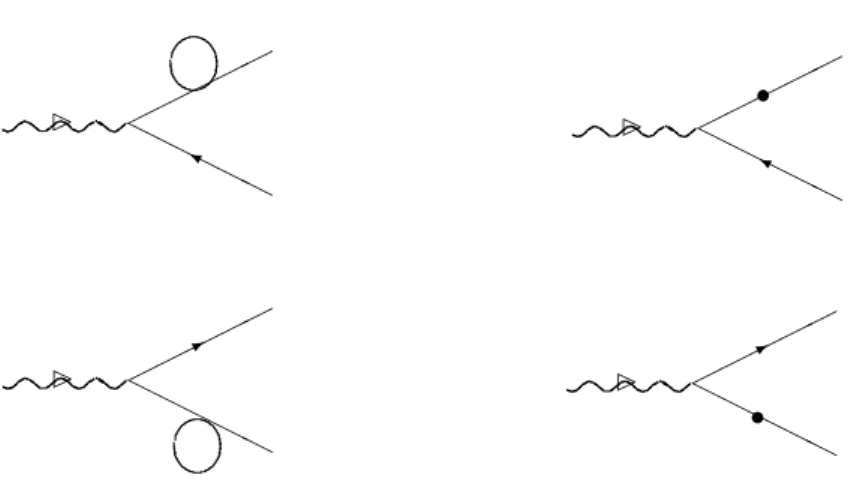
TµνSVV(k1,k2,k3;m) = Z d4k
(2π)4Tr
½
b1 1
(6k+6k3)−mγµ 1
(6k+6k1)−mγν 1 (6k+6k2)−m
¾
. (31)
(a) 1
γµ
γν k+k3
k+k1 k+k2
✯
❨ ❄
•
• •✟✟
✟✟
❍ ❍
❍❍
(b)
• •
✛ ✲
k+ki
k+kj
1 γµ
Figure 4: Diagrammatic representation for theSVVthree-point function and for theSVtwo-point function, Figs.(a) and (b) respectively.
Contracting with the vector’s vertexes momenta we can obtain a condition for the corresponding Ward identities
(k3−k1)µTµνSVV =
Z d4k (2π)4Tr
½
ˆ1 1
(6k+6k1)−mγν 1 (6k+6k2)−m
¾
(32)
− Z d4k
(2π)4Tr
½
ˆ1 1
(6k+6k3)−mγν 1 (6k+6k2)−m
¾
,
where we have used in the traces level the identity
(6k3− 6k1) = [6k+6k3−m]−[6k+6k1−m]. (33) Let us now define the two-point function of the right hand side as (see Fig.4(b))
TµV S(k1,k2;m) = Z d4k
(2π)4Tr
½
γµ 1 (6k+6k1)−mˆ1
1 (6k+6k2)−m
¾
,
(34) and
TµνS→VV =TµνSVV(k1,k2,k3;m) +TνµSVV(l1,l2,l3;m), (35)
in order to write the Ward identities as
pµTµνS→VV = TνV S(k1,k2;m)−TνV S(k3,k2;m) +TνV S(l3,l2;m)−TνV S(l3,l1;m) (36) p′νTµνS→VV = TµV S(k3,k2;m)−TµV S(k3,k1;m) +TνV S(l1,l2;m)−TνV S(l3,l2;m). (37) The conditions for the symmetry relations maintenance are put in terms of the value for theSV two-point function structure. If the traces involved are performed we get
TµV S = 4m
½Z d4k
(2π)4
2kµ
[(k+k1)2−m2][(k+k2)2−m2] +(k1+k2)µ
Z d4k (2π)4
1
[(k+k1)2−m2][(k+k2)2−m2]
¾
which means that
TµV S=4m
n
(k1+k2)µI2+2(I2)µ
o
, (39)
or, given the definition (23),
TµV S=4m(∆Iµ). (40) If we look at the equation (22) of the preceding section we can see that the condition we have found for the Ward identities involved in theS→VV process is the same one we found for the complex scalar theory Ward identity. Only if the structure (40) is obtained identically vanishing, the symmetry relations are preserved by the one-loop perturbative calculation. Before the analysis let us now consider another (and more interesting) set of symmetry relations.
IV. A→VV PROCESS
A more interesting situation involving Ward identities emerges when we want to consider the process where an
Axial-Vector is connected with two vectors. Such a process can be constructed by coupling the appropriate fermionic den-sities with the external fields. Similar discussions can be found in the ref.[11] (see also ref.[10] and [12]). The inter-action Lagrangian can be written as
L
I =iGP(Ψγ¯ 5Ψ)π−eV¡¯
ΨγµΨ¢Aµ−eA
¡¯
Ψγ5γµΨ
¢
WµA. (41) Here,Ψis the massive12fermion,WµAis an Axial-Vector field andπis a pseudo-scalar one. The fermionic currents obey
½
∂µVµ=∂µ
¡¯
ΨγµΨ¢=0
∂µAµ=∂µ
¡¯
Ψγ5γµΨ
¢
=2mi(Ψγ¯ 5Ψ) =2miP. . (42)
In such theory we can define the Green’s functions
TµνλA→VV(p,p′;q) = i Z
d4x1d4x2 eipx1+ip′x2<0|T(Vµ(x1)Vµ(x2)A
λ(0))|0>, (43)
TµνP→VV(p,p′;q) = i Z
d4x1d4x2 eipx1+ip
′x
2<0|T(V
µ(x1)Vν(x2)P0(0))|0> . (44)
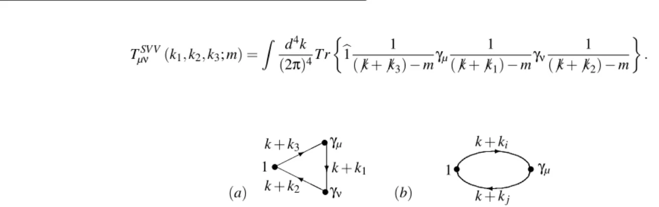
The standard procedure of current algebra can be used to state the Ward identities
p′νTλµνA→VV = 0, (45)
pµTλµνA→VV = 0, (46)
qλTλµνA→VV = 2mTµνP→VV. (47)
The lowest order perturbative calculation of theAVV process requires the evaluation of the one-loop triangle diagrams of the Fig.5(a) and (b). The definitions for the external and inter-nal lines follow the same conventions of the preceding section. So, we write for the direct channel (see Fig.5(a))
TλµνAVV(k1,k2,k3;m) = Z d4k
(2π)4Tr
½
iγλγ5 1
(6k+6k3)−mγµ 1
(6k+6k1)−mγν 1 (6k+6k2)−m
¾
. (48)
(a) iγλγ5
γµ
γν k+k3
k+k1 k+k2
✯
❨ ❄
•
• •✟✟
✟✟
❍ ❍
❍❍
(b) γ5
γµ
γν k+k3
k+k1 k+k2
✯
❨ ❄
•
• •✟✟
✟✟
❍ ❍
❍❍
(c)
• •
✛ ✲
k+ki
k+kj
iγµγ5 γν
Figure 5: Diagrammatic representation for theAVV andPVV three-point functions and for theAV two-point function, Figs.(a), (b) and (c), respectively.
Contracting with the external momenta we can derive con-ditions to be fulfilled in order to get the respective Ward
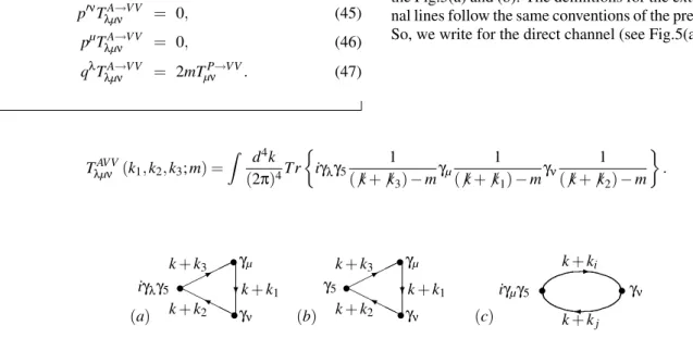
(k3−k2)λand use the identity
(6k2− 6k3)γ5= (6k+6k2−m)γ5+γ5(6k+6k3−m)+2mγ5, (49)
in the interior of the traces, to get
(k3−k2)λTλµνAVV = −2mi Z d4k
(2π)4Tr
½
γ5 1 [6k+6k3−m]
γµ 1 [6k+6k1−m]
γν 1
[6k+6k2−m]
¾
− Z d4k
(2π)4Tr
½
iγνγ5 1 [6k+6k3−m]
γµ 1 [6k+6k1−m]
¾
+ Z d4k
(2π)4Tr
½
iγµγ5 1 [6k+6k1−m]
γν 1
[6k+6k2−m]
¾
. (50)
If we define the two-point functions on the right hand side as (see Fig. 5(c))
TξρAV(ki,kj;m) = Z d4k
(2π)4Tr
½
iγξγ5 1 (6k+6ki)−mγρ
1 (6k+6kj)−m
¾
, (51)
we can write (see Fig.6)
(k3−k2)λTλµνAVV=−2imTµνPVV−TνµAV(k3,k1;m) +TµνAV(k1,k2;m), (52) where we have defined (seeFig.5(b))
TµνPVV(k1,k2,k3;m) = Z d4k
(2π)4Tr
½
γ5 1
(6k+6k3)−mγµ 1
(6k+6k1)−mγν 1 (6k+6k2)−m
¾
. (53)
(k3−k2)λ iγλγ5
γµ
γν k+k3
k+k1 k+k2
✯
❨ ❄
•
• •✟✟
✟✟
❍ ❍
❍❍
=−2im γ5
γµ
γν k+k3
k+k1 k+k2
✯
❨ ❄
•
• •✟✟
✟✟
❍ ❍
❍❍
+ • •
✛ ✲
k+k1
k+k2
iγµγ5 γν − • •
✛ ✲
k+k3
k+k1
iγνγ5 γµ
Figure 6: Diagrammatic representation for the identity(52).
Now if we take the contractions of theAVV function with the vector’s momenta we immediately identify (see Fig.7)
(k3−k1)µTλµνAVV =TλνAV(k1,k2;m)−TλνAV(k3,k2;m). (54) Also, in a similar way we can state (see Fig.8)
(k1−k2)νTλµνAVV =TλµAV(k3,k2;m)−TλµAV(k3,k1;m). (55)
(k3−k1)µ iγλγ5
γµ
γν k+k3
k+k1 k+k2
✯
❨ ❄
•
• •✟✟
✟✟
❍ ❍
❍❍
= • •
✛ ✲
k+k1
k+k2
iγλγ5 γν − • •
✛ ✲
k+k3
k+k2
iγλγ5 γν
Figure 7: Diagrammatic representation for the identity (54).
(k1−k2)ν iγλγ5
γµ
γν k+k3
k+k1 k+k2
✯
❨ ❄
•
• •✟✟
✟✟
❍ ❍
❍❍
= • •
✛ ✲
k+k3
k+k2
iγλγ5 γµ − • •
✛ ✲
k+k3
k+k1
iγλγ5 γµ
The inclusion of the crossed channel allows us to write the following expressions
qλTλµνA→VV = −2imTµνP→VV+TµνAV(k1,k2;m)−TνµAV(k3,k1;m) +TνµAV(l1,l2;m)−TµνAV(l3,l1;m), (56) pµTλµνA→VV = TλνAV(k1,k2;m)−TλνAV(k3,k2;m) +TλνAV(l3,l2;m)−TλνAV(l3,l1;m), (57) p′νTλµνA→VV = TλµAV(k3,k2;m)−TλµAV(k3,k1;m) +TλµAV(l1,l2;m)−TλµAV(l3,l2;m). (58) The conditions for Ward identities preservation are now put in terms of theAV two-point functions. They are the same ones we can find in the ref.[10], [11] and [12]. The evaluation of the traces leads us to the expression
TµνAV(k1,k2;m) = −4εµναβ
½
kβ2 Z d4k
(2π)4
kα
[(k+k1)2−m2][(k+k2)2−m2] +kα1
Z d4k (2π)4
kβ
[(k+k1)2−m2][(k+k2)2−m2] +k1αkβ2
Z d4k (2π)4
1
[(k+k1)2−m2][(k+k2)2−m2]
¾
. (59)
We can use the properties of the totally antisymmetric tensor εµναβin order to put the equation above into the form
TµνAV(k1,k2;m) =2εµναβ(k1−k2)β
©
(k1+k2)αI2+2(I2)α
ª
. (60) This means that, given the definition (23), we have
TµνAV(k1,k2;m) =2εµναβ(k1−k2)β(∆Iα), (61) which means that the condition is the same one as those found in the preceding sections. Now it is time to study the divergent integrals that appeared in the three amplitudes considered and their symmetry relations.
V. THE CALCULATIONAL STRATEGY
If the explicit evaluation of perturbative (divergent) ampli-tudes is in order we need to specify some philosophy to handle the mathematical indefinitions involved. Usually the calcula-tions become reliable only after the adoption of a regulariza-tion technique. After this, in the intermediary steps, we invari-ably assume some specific consequences for the results intrin-sically associated to the properties attributed for the divergent integrals resulting from the (arbitrary) choices for the math-ematical indefinitions implied by the adopted regularization. In the final form this way obtained, for the amplitudes in gen-eral, it is not possible to specify in a clear way what are the particular effects of the adopted regularization for the result or, in other words, to evaluate in what sense the expression is dependent on the adopted technique. In order to perform a as safe as possible analysis of the properties of the divergent am-plitudes, including their symmetry relations and the question of the ambiguities related to the arbitrariness involved in the routing of the loop internal lines momenta, we need to avoid as much as possible specific choices in the intermediary steps so that all the possibilities still remain contained in the final results. If it is possible, we can change the usual focus of the analysis, which is the verification by testing the consistency of
the proposed regularization technique, for the identification of the eventual properties such a technique should have in order to be consistent. The implication of the preceding arguments, which will become clear in what follows, will play an impor-tant role in the discussion we want to perform.
To explicitly evaluate the divergent integrals involved we will adopt an alternative strategy to handle the divergences. The referred method, introduced in ref. [7], has been used recently in the literature in different contexts. It allows us a clear and universal point of view for the divergences of per-turbative calculations in QFT. The strategy is simple: instead of the specification of some regularization, to justify all the necessary manipulations, we will assume the presence of a regulating distribution only in an implicit way. Schematically
Z d4k
(2π)4f(k) →
Z d4k (2π)4f(k)
(
lim Λ2
i→∞ GΛi
¡
k,Λ2i
¢)
= Z
Λ d4k
(2π)4f(k). (62) HereΛ′
isare parameters of the generic distributionG(Λ2i,k) that, in addition to the obvious finite character of the modified integral, must have two other very general properties. It must be even in the integrating momentumk, due to Lorentz invari-ance mainteninvari-ance, as well as a well-defined connection limit must exists, i.e.,
lim Λ2
i→∞ GΛi
¡
k2,Λ2 i
¢
=1. (63)
identity like
1 [(k+ki)2−m2]
= N
∑
j=0(−1)j¡k2i+2ki·k¢j (k2−m2)j+1 + (−1)
N+1¡
ki2+2ki·k
¢N+1
(k2−m2)N+1h(k+k i)2−m2
i,(64)
wherekiis (in principle) an arbitrary choice for the routing of a loop internal line momentum. The value for N must be ad-equately chosen. The minor value must be the one that leads
the last term in the above expression to be present in a finite integral and therefore, by virtue of the well-defined connec-tion limit assumpconnec-tions, the corresponding integraconnec-tion can be performed without any restrictions and free from the specific effects of the eventual regularization. All the remaining struc-tures become independent on the internal lines momenta. We then eliminate all the integrals with odd integrand, as a trivial consequence of the even character of the regulating implicit distribution. In the divergent structures obtained this way no additional assumptions are taken. They are organized in five objects, namely
¤αβµν = Z
Λ d4k (2π)4
24kµkνkαkβ (k2−m2)4 −gαβ
Z
Λ d4k (2π)4
4kµkν
(k2−m2)3 (65)
−gαν Z
Λ d4k (2π)4
4kβkµ
(k2−m2)3−gαµ Z
Λ d4k (2π)4
4kβkν (k2−m2)3,
∆µν = Z
Λ d4k (2π)4
4kµkν (k2−m2)3−
Z
Λ d4k (2π)4
gµν
(k2−m2)2, (66)
∇µν = Z
Λ d4k (2π)4
2kνkµ (k2−m2)2−
Z
Λ d4k (2π)4
gµν
(k2−m2), (67)
Ilog(m2) = Z
Λ d4k (2π)4
1
(k2−m2)2, (68)
Iquad(m2) = Z
Λ d4k (2π)4
1
(k2−m2). (69)
This systematization is sufficient for discussions in fundamen-tal theories at the one-loop level. In the non-renormalizable ones new objects can be defined following this philosophy. In the two (or more) loop level of calculations new basic diver-gent structures can be equally defined in a completely analo-gous way. The main point is to avoid the explicit evaluation of such divergent structures in which case a regulating distri-bution needs to be specified.
We can say that this procedure furnishes an universal point of view for the calculated amplitudes since it become possible to map the final expressions obtained this way into the corre-sponding results of other techniques. All the steps followed and all the assumptions are perfectly valid in the reasonable regularization prescriptions, including the DR. All we need, to extract from our results those of a specific technique, is to evaluate the divergent structures, remaining at the final expres-sion, according to the specific chosen prescription. Another important fact we call the attention is that no shifts or expan-sions are used in the intermediary steps. We assume the more general routing for all amplitudes. The potentially ambiguous terms are still present in the final result. Consequently, it is possible to make contact with those results corresponding to explicit evaluation of surface’s terms involved when shifts in the integrating momenta are performed. This is an important
aspect of our analysis because we want to make contact with the traditional approach used to justify the triangle anomalies. In order to clarify the above described method, to handle the divergences, let us apply the calculational strategy in the treat-ment for some divergent integrals. For this purposes we take two of them that will play an important role in our analysis. They are two-point function structures defined in eq.(24). The I2integral, is a logarithmically divergent structure while(I2)µ is linearly divergent. In this structuresk1andk2represents, in principle, arbitrary choices for the internal lines momenta. Then we can expect a dependence onk1andk2other than the difference between them only for the(I2)µintegral.
Taken first theI2 integral we choose, in the identity (64), N=1 to rewrite both denominators. Then we get
I2 = Z
Λ d4k (2π)4
1
(k2−m2)2 (70)
− Z d4k
(2π)4
(k12+2k1·k)2 [(k2−m2)2][(k+k
1)2−m2] −
Z d4k (2π)4
(k22+2k2·k)2 [(k2−m2)2][(k+k
2)2−m2] +
Z d4k (2π)4
(k21+2k1·k)(k22+2k2·k)
The right hand side exhibits the desirable form. The divergent term is located in an internal momenta independent structure which we can identify asIlog
¡
m2¢, defined in eq.(68). The remaining structures are finite ones and we use what we call the connection limit existence to drop theΛsubscript on the integral, or, equivalently, to remove the eventual regulating distribution under the argumentation that the integration and the connection limit can be perfectly interchanged. The thus obtained finite Feynman integrals can be solved without any problem. The answer can be written as
I2=Ilog(m2)−
µ
i (4π)2
¶
Z0((k1−k2)2;m2), (71) where we have introduced (in short hand notation) the two-point functions structures [7]
Zk(λ21,λ22,q2;λ2) = Z 1
0 dzzkln
µ
q2z(1−z) + (λ2
1−λ22)z−λ21 (−λ2)
¶
.
(72)
Integration over parameterzcan be easily performed however for our present purposes this is not necessary.
Following the procedure we can evaluate also theI2µ inte-gral. The first step is the same: the use of the identity (64) to rewrite the integrand, now to the form
(I2)µ=− 1
2(k1+k2) αZ
Λ d4k (2π)4
4kαkµ
(k2−m2)3 (73) +
Z d4k (2π)4
(k12+2k1·k)2kµ [(k2−m2)3][(k+k
1)2−m2] +
Z d4k (2π)4
(k22+2k2·k)2kµ [(k2−m2)3][(k+k
2)2−m2] +
Z d4k (2π)4
(k2
1+2k1·k)(k22+2k2·k)kµ [(k2−m2)2][(k+k
1)2−m2][(k+k2)2−m2]
.
In the above expression, we have dropped two oddkintegrals, by virtue of the even character of the implicit regulating dis-tribution as well as theΛsubscript in the last three terms due
to the finite character. After the integration of the finite terms we are lead to the result
(I2)µ = − 1
2(k1+k2) α(∆
αµ)−1
2(k1+k2)µ
©
Ilog(m2) −
µ
i (4π)2
¶
Z0((k1−k2)2;m2)
¾
= −1
2(k1+k2) α(∆
αµ)− 1
2(k1+k2)µ(I2).
It is important, at this point, to emphasize the general aspects of the method. No shifts has been performed and, in fact, no divergent integrals calculated. All the final results produced by this approach can be mapped in those of any specific tech-nique. The finite parts are the same as should be by physical reasons. The divergent parts can be easily obtained. All we need is to evaluate the remaining divergent structures accord-ing to the chosen prescription. By virtue of this general char-acter, the present strategy can be used simply to systematize the procedures, even if one wants to use traditional techniques. Let us now to use the above obtained results to calculate the physical amplitudes involved in our present discussions.
VI. DIVERGENCES, AMBIGUITIES AND WARD IDENTITIES
Given the results obtained in the preceding section we can evaluate the combination of Feynman integrals which revealed being crucial for all the Ward identities we have studied. Sub-stituting the results (71) and (74) in the expression (23) we get
∆Iµ= (k1+k2)α(△αµ), (74) and consequently,
TµV S(k1,k2;m) = −4m(k1+k2)α(△αµ), (75) TµνAV(k1,k2;m) =2εµναβ(k1−k2)α
n
(k1+k2)ξ
³
△βξ´o(76).
The Ward identities we studied in the sections II, III and IV can be written into the following form
iqµΓ1loopµ (p,q) = iλ(k1−k2)µ(k1+k2)α(△αµ), (77) qλTλµνA→VV = −2mi[TµνP→VV] +2εµναβ
h
(k1−k3)β(k1+k3)ξ+ (k2−k1)β(k1+k2)ξ
i ³
△αξ´ (78)
−2εµναβ
h
(l1−l3)β(l1+l3)ξ+ (l2−l1)β(l1+l2)ξ
i ³
△αξ´,
pµTλµνA→VV = 2ελναβ
h
(k2−k1)β(k1+k2)ξ+ (k3−k2)β(k2+k3)ξ
i ³
△αξ´ (79)
+2ελναβ
h
(l3−l1)β(l1+l3)ξ+ (l2−l3)β(l2+l3)ξ
i ³
p′νTλµνA→VV = 2ελµαβ
h
(k3−k1)β(k1+k3)ξ+ (k2−k3)β(k2+k3)ξ
i ³
△αξ´ (81)
+2ελµαβ
h
(l2−l1)β(l1+l2)ξ+ (l3−l2)β(l2+l3)ξ
i ³
△αξ´,
pµTµνS→VV = 4m(k3−k1)ξ
¡
△ξν
¢
+4m(l1−l2)ξ
¡
△ξν
¢
=8mpξ¡△ξν
¢
, (82)
p′νTλµνS→VV = 4m(k1−k2)ξ
¡
△ξµ
¢
+4m(l3−l1)ξ
¡
△ξµ
¢
=8mp′ξ¡△ξµ
¢
. (83)
There are two types of undefined quantities in the expressions above. This means that in order to get definite results for the involved amplitudes it becomes necessary to assume some (ar-bitrary) choices for them. Such choices must be obviously guided by the consistency we want to get in perturbative cal-culations, in spite of the divergent character. Having this in mind we can ask for the existence of eventual physical con-straints to be used in order to get the adequate choices for the arbitrariness present in the results above. Clearly, there are two types of constraints which we must fulfill. The first
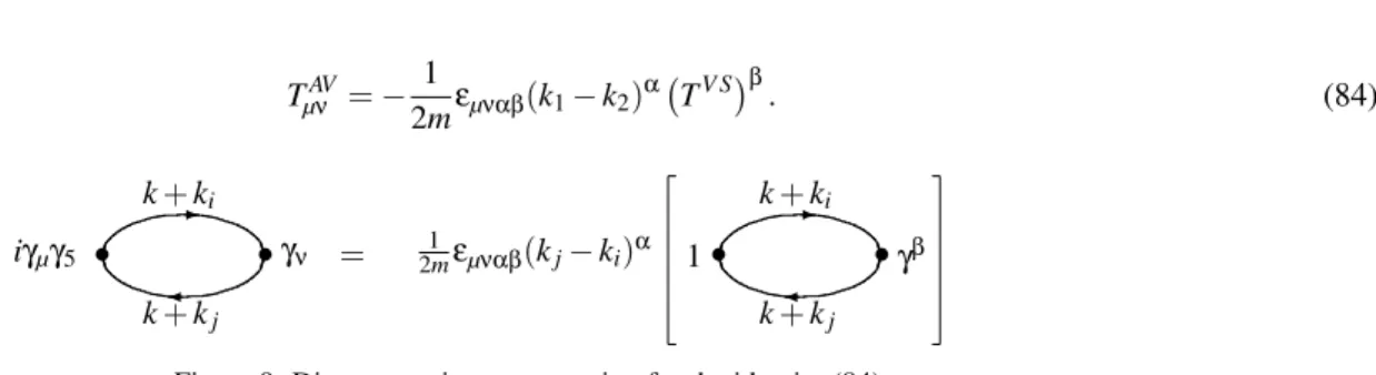
one refers to the Ward identities themselves, i.e., we want to make choices that lead, in principle, to their preservation. For the second, we cannot forget that the conditions (78)-(83) are obtained after the evaluation of theAVandSVtwo-point func-tions, so that our choices for the arbitrariness must not imply in non-physical results for these amplitudes. In addition, we note that these two amplitudes are deeply related. There is an identity at the traces level relating them, namely (see Figure 9):
TµνAV=− 1
2mεµναβ(k1−k2)
α¡TV S¢β.
(84)
=
• •
✛ ✲
k+ki
k+kj
iγµγ5 γν 2m1 εµναβ(kj−ki)α • •
✛ ✲
k+ki
k+kj
1 γβ
Figure 9: Diagrammatic representation for the identity (84).
The identity is valid before any calculations have been made, i.e., independent of the divergences related aspect in-volved. It must be valid after all the calculations are per-formed independent of the adopted regularization philosophy. Within our calculational strategy, the above identity is pre-served before any choices for the arbitrariness involved. Both amplitudes are, in principle, ambiguous quantities. The iden-tity (84) is not ambiguous and should be maintained after the adopted interpretations for the arbitrariness involved. Given this observation it is natural to start by the analysis of the SV andAV two-point functions. First, by unitarity reasons (Cutkosky’s rules), both two-point functions should have an imaginary part arising at the kinematical point(k1−k2)2= 4m2. If a nonzero value for the referred amplitudes is at-tributed, independent of the possible choices involved, such a threshold will not be present. For the second, Lorentz and CPT arguments also require the vanishing value. Otherwise, a transition between a vector into a scalar particle and be-tween an axial into a vector particle seems to be possible through theSV andAV two-point functions respectively. We can also add some arguments coming from Ward identities. The SV amplitude carries a vector Lorentz index in such a way the contraction with the external momentum of the
re-spective vertex should vanish, in order to maintain the vector current conserved. Given the expression (76), the contraction with(k1−k2)µgives us
(k1−k2)µTµV S=−4m(k1−k2)µ(k1+k2)ξ[△ξµ], (85) which is not automatically zero. On the other hand, theAV amplitude should also exhibit a conserved vector current. The contraction of the expression (77) with(k1−k2)µ, due to the symmetry properties of theεµναβtensor, gives us
(k1−k2)µTµνAV =0. (86) This is therefore a good property. However, by the same rea-sons put above, we get
Given this conclusion the question immediately raised is: how can we use the arbitrariness remaining in the expressions (76) and (77) in order to obtain the desirable results? Looking at the structure of the results (76) and (77) we see that there are two basic possibilities. First, due to the fact that the value for k1+k2 is not fixed by the energy-momentum conservation, we can choosek1=q/2 andk2=−q/2 whereqis the exter-nal momentum. Within this procedure the value for the object ∆µνis not constrained and all regularizations can be used to evaluate it. Secondly, since we need to calculate the value for ∆µν, i.e., to adopt a regularization, we can select it in such a way that∆regµν=0. Both choices should impose a price to be paid in other calculations if we want to construct a procedure, i.e., if we assume that all the amplitudes in all theories and models must be treated in the same way. The first possibility pointed above implies in the assumption that the amplitudes may emerge ambiguous from the calculations, i.e., dependent on the choices for the internal lines labels. This is bad because the predictive power of QFT in the perturbative approach is destroyed and, as a consequence, we can use the theory only to produce adjustments to well-known phenomenologies. The predictions cannot be stated in general because the amplitudes may have undefined pieces. In addition, in adopting this way, we are assuming that the space-time homogeneity is broken in the calculations. If, on the other hand, we take the second op-tion there are also some implicaop-tions. Specific properties for the divergent integrals are assumed and they need to be used in all other calculations with the same value and exhibiting the same consistency, which, in fact, should be verified.
After these important remarks we return to the Ward identi-ties (78)-(83). Looking at the Ward identiidenti-ties for the complex scalar field we note that there are two types of arbitrariness involved; the presence of the undefined piece∆and the am-biguous combination of the external lines momentak1+k2. We have both options described above in order to get a sym-metry preserving result. A different situation occurs in the SVV symmetry relation. Even that the condition for the sym-metry preservation was put in terms of four potentially am-biguous terms they appear in non-amam-biguous combinations. So all the choices for the internal arbitrary momenta lead us to the same result. Only the choice∆regµν =0 will give us the desirable result. We note that these two problems, the scalar field andSVV process, can be treated within the DR. In fact, the strategy we have used to perform the calculations, with the
choice∆regµν =0, becomes identical to the DR in theories with only bosonic fields and mappable one-by-one in theories with fermions. TheSV amplitude is trivially obtained identically zero in the DR. Then, it seems obvious that all the physical requirements are fulfilled by the choice∆regµν =0, which maps the DR results. What are the reasons for hesitation in assum-ing this option? The answer can be extracted from the conse-quences of this choice for the Ward identities (78)-(83): they become
iqµΓ1loopµ (p,q) = 0, (88) p′νTµνS→VV = 0, (89) pµTµνS→VV = 0, (90) and
p′νTλµνA→VV = 0, (91)
pµTλµνA→VV = 0, (92)
qλTλµνA→VV = −2miTµνP→VV, (93) i.e., all the Ward identities become preserved and all the ambi-guities are automatically eliminated. At first sight this fact can be understood as a trouble because, apparently, we are forbid-ding any violation of symmetry relations in theAVV triangle amplitude which is well known should present an anomaly to be consistent with the electromagnetic pion decay. At least this is the line of reasoning which we can find in the tradi-tional literature about this issue. In order to justify the anom-aly it is assumed that the undefined terms on the right hand side of the eqs.(79)-(81), which are in the last instanceAV physical amplitudes, are non-vanishing and ambiguous. In or-der to make clear the last sentence let us consior-der the recover-ing of the results correspondrecover-ing to what we call the traditional treatment from the ones of the adopted calculational strategy. The referred results can be easily found in the literature about the subject or in many textbooks of QFT. It is a very simple job to pass from our results to the ones corresponding to the surface’s terms evaluation due to the fact that no shifts have been made in the intermediary steps. All we need is: first to state the identities (55)-(57), and then to evaluate the two-point function structures thus obtained, with the help of the results (71) and (74), which lead us to the expression
(k3−k2)λTλµνAVV = −2mi[TµνPVV] +2εµναβ
h
(k1−k3)β(k1+k3)ξ+ (k2−k1)β(k1+k2)ξ
i ³
△αξ´, (94)
(k3−k1)µTλµνAVV = 2ελναβ
h
(k2−k1)β(k1+k2)ξ+ (k3−k2)β(k2+k3)ξ
i ³
△αξ´, (95)
(k1−k2)νTλµνAVV = 2ελµαβ
h
(k3−k1)β(k1+k3)ξ+ (k2−k3)β(k2+k3)ξ
i ³
△αξ´. (96)
Now we observe that, in order to give a definite value for the right hand side of the equations, two types of arbitrariness
un-defined mathematical object. The difference between two log-arithmically divergent integrals, however, can be immediately identified with a typical surface’s term and easily evaluated as follows
∆Sµν = Z
Λ d4k (2π)4
∂ ∂kν
Ã
kµ (k2−m2)2
!
= Z
Λ d4k (2π)4
−4kµkν (k2−m2)3+
Z
Λ d4k (2π)4
gµν (k2−m2)2 =
Ã
i (4π)2
! µ
1 2
¶
gµν.
Note that the same result could be obtained by shifting the integrating momentum in one of the two-point function struc-tures in order to produce a cancellation with the other one. The price to be paid, which is well known, is the addition of the corresponding surface’s term which assumes exactly the value obtained above. The next step is the removal of the un-defined combination of internal momenta. We adopt then a parametrization for the internal momenta in terms of the ex-ternal ones
k1=ap′+bp k2=bp+ (a−1)p′ k3=ap′+ (b+1)p.
(97)
whereaandbare constants. Notice that : k1−k2=p′,k3− k1= p andk3−k2=p′+p=q, where q is obviously the momentum of the axial vector. After these substitutions we get
(k3−k2)λTλµνAVV =−2miTµνPVV− (a−b)
8π2 iεµνξηp ′ηpξ,
(98)
(k3−k1)µTλµνAVV = − (1−a)
8π2 iελνξηp
′ηpξ, (99) (k1−k2)νTλµνAVV =
(1+b) 8π2 iελµξηp
′ηpξ. (100)
In the expressions above it remains the arbitrariness related to the routing of internal lines now present in the parametersa andb. In addition we note that there are no values foraand bin such a way that all the expected relations among the in-volved Green’s functions are simultaneously satisfied. If we follow this line of reasoning and include the contribution of the crossed diagram whose parametrization for the internal lines momenta can be assumed as
l1=cp+d p′ l2=d p′+ (c−1)p l3=cp+ (d+1)p′,
(101)
we will obtain
(l3−l2)λTλνµAVV =−2miTνµPVV− (c−d)
8π2 iεµνξηp
′ηpξ,(102) (l1−l2)µTλνµAVV = −
(d+1) 8π2 iελνξηp
′ηpξ, (103)
(l3−l1)νTλνµAVV = − (c−1)
8π2 iελµξηp ′ηpξ.
(104)
The addition of the two contributions gives us
qλTλµνA→VV =−2miTµνP→VV−(a−b+c−d) 8π2 iεµνξηp
′η(105)pξ,
pµTλµνA→VV = −(d−a+2) 8π2 iελνξηp
′ηpξ,
(106)
p′νTλµνA→VV = −(c−b−2) 8π2 iελµξηp
′ηpξ.
(107)
A closer contact with the usual results can be obtained if it is assumed the same significance for the arbitrary internal mo-menta, i.e.,a=candb=din the eqs.(56)-(58).We get then
qλTλµνA→VV = −2miTµνP→VV−(a−b) 4π2 iεµνξηp
′ηpξ, (108)
pµTλµνA→VV = −(b−a+2) 8π2 iελνξηp
′ηpξ,
(109)
p′νTλµνA→VV = (b−a+2) 8π2 iελµξηp
′ηpξ. (110)
Finally, we choose the valuea=1 in the above expression to get
qλTλµνA→VV = −2miTµνP→VV−(1−b) 4π2 iεµνξηp
′ηpξ,(111)
pµTλµνA→VV = −(1+b) 8π2 iελνξηp
′ηpξ, (112)
p′νTλµνA→VV = (1+b) 8π2 iελµξηp
′ηpξ. (113)
The result this way obtained, can be immediately recognized as the traditional one [2],[10], [11], [12]. It is now clear that there is no value for thebparameter in order to preserve all Ward identities. Following the usual arguments and choosing the valueb=−1 theU(1)gauge symmetry is maintained, but the axial one is violated. Which have become clear in the discussion above is that the sources of the violating terms as well as of the anomalous term areAV two-point function structures.
VII. FINAL REMARKS AND CONCLUSIONS
all the ambiguities in theAVV amplitude which are the ingre-dients usually used to justify the anomaly involved, and, ap-parently, forbids any violation of symmetry relations for this amplitude. How can we reconciliate this situation? In order to answer this question it is necessary to assume a conceptual and philosophical point of view for the problem: the tradi-tional way used to justify the AVV triangle anomaly cannot be maintained if we want to look at all the problems in the same way and the ambiguities cannot play a relevant role in a consistent interpretation of the perturbative amplitudes. In this line of reasoning we first need to break fundamental sym-metries and general principles of QFT, by assuming the SV andAV structures as non-vanishing ones, for only after this get a justification for the perturbative origin of the anomalies. A powerful philosophical argument can be added to these ob-jective ones. TheAVV anomaly phenomenon is predicted for the exact amplitudes, i.e., it is a fundamental phenomenon. However, in the eventual exact solutions for the correspond-ing QFT‘s equations of motion certainly the infinities and the associated ambiguities must be absent. So, we cannot expect that the justification of the origin of the anomaly phenomenon, even in perturbative solutions, resides in exclusive ingredients of the perturbative calculations as the infinities and ambigui-ties are. Given this argument, the answer for the question put above is intrinsically contained in the problem. Being a fun-damental and unavoidable phenomenon, the anomaly should be present in any explicit expression for theAVV amplitude. This means that no choices for the arbitrariness can eliminate the anomaly as well as no regularization prescription or equiv-alent philosophy. Then we can expect that a point of view for the anomalies can be constructed in accordance with all the others in perturbative calculations. For this purposes it is necessary to evaluate explicitly theAVV andPVV
ampli-tudes imposing the consistency condition, and expecting that the violations emerge in a natural way. Which have become clear in the discussions presented here is that in the context of traditional regularization procedures different prescriptions are used for the treatment of identical mathematical structures depending on the context they appear.
The present status of the problem can be summarized as follows. In the situations where the DR can be used, elimi-nating the ambiguities, we certainly adopt it. In the situations where the involving mathematical structures are not naturally extendable to any dimension, which is the case of triangle anomalies, we adopt the surface’s terms evaluation, attributing a meaning to the ambiguous character of the perturbative am-plitudes. In a certain way, in situations where these problems do not simultaneously occur this option represents a possible choice for the involved arbitrariness. However, admitting the intention of looking at all the fundamental interactions as parts of a more general and unified theory, it seems a patently ab-surd idea because this means that in a certain amplitude of the same theory a value is attributed for the objects△µν, having in mind consistency reasons, while in other amplitudes the value can be taken as different without any crisis of conscience. Cer-tainly it would be very frustrating for any physicist who got interested in studying an exact science to accept this situa-tion as a final one. This situasitua-tion is clearly unacceptable and additional efforts in order to achieve consistent and universal interpretations for the mathematical indefinitions intrinsic of the perturbative calculations are required. The strategy de-scribed in the section V seems to put the analysis in the right direction.
Acknowledgements: G.D. and O.A.B acknowledges a grant from CNPq/Brazil. E.G. acknowledges a grant from CAPES/Brazil.
[1] G.’t Hooft and M. Veltman, Nucl. Phys. B44189 (1972); C.G. Bollini and J.J. Giambiagi, Phys. Lett. B40 566 (1972); J.F. Ashmore, Nuovo Cimento Lett.4289 (1972).
[2] J. S. Bell and R. Jackiw, Nuovo Cim. A60,47 (1969). [3] S. Adler, Phys. Rev.177, 2426 (1969).
[4] S. Adler and W.A. Bardeen, Phys. Rev.182, 1517 (1969); W.A. Bardeen, Phys. Rev.184, 1848 (1969).
[5] I.S. Gerstein and R. Jackiw, Phys. Rev.181, 1955 (1969). [6] V. Elias, Gerry McKeon, R.B. Mann, Nucl. Phys. B229 487
(1983).
[7] O.A. Battistel,PhD Thesis (1999), Universidade Federal de Mi-nas Gerais, Brazil.
[8] O.A. Battistel and G. Dallabona, Phys. Rev. D65, 125017 (2002).
[9] O.A. Battistel and O.L. Battistel, Int. J. Mod. Phys. A17, 1979-2017 (2002).
[10] T.P. Cheng and L.F. Li,Gauge Theory of Elementary Particle Physics, Oxford University Press, New York (1984).
[11] P.H. Frampton,Gauge Field Theories Benjamin /Cummings, Menlo Park, California (1987).