Scaling Properties of the Fermi-Ulam Accelerator Model
Jafferson Kamphorst Leal da Silva, Denis Gouvˆea Ladeira, Departamento de F´ısica, ICEx, Universidade Federal de Minas Gerais,
Caixa Postal 702, 30.123-970 Belo Horizonte, MG, Brazil
Edson D. Leonel,
Departamento de Estat´ıstica, Matem´atica Aplicada e Computac¸˜ao,
Universidade Estadual Paulista Julio de Mesquita Filho, 13506-700 Rio Claro, SP, Brazil
P. V. E. McClintock,
Department of Physics, Lancaster University, LA1 4YB, United Kingdom
and Sylvie O. Kamphorst
Departamento de Matem´atica, Instituto de Ciˆencias Exatas,
Universidade Federal de Minas Gerais, C. P. 702, 30123-970 Belo Horizonte, MG, Brazil
Received on 25 October, 2005
The chaotic low energy region (chaotic sea) of the Fermi-Ulam accelerator model is discussed within a scaling framework near the integrable to non-integrable transition. Scaling results for the average quantities (velocity, roughness, energy etc.) of the simplified version of the model are reviewed and it is shown that, for small oscillation amplitude of the moving wall, they can be described by scaling functions with the same characteristic exponents. New numerical results for the complete model are presented. The chaotic sea is also characterized by its Lyapunov exponents.
Keywords: Fermi Model; Chaos; Lyapunov Exponent; Scaling
I. INTRODUCTION
The Fermi accelerator model is a one-dimensional system originally proposed by Fermi in 1949 [1] to study cosmic rays. It provides a mechanism through which a charged par-ticle can be accelerated by collision with a time-dependent magnetic field. Since then, different versions of this model have been proposed and studied by several authors. One of them is the so called Fermi-Ulam model (FUM), which con-sists of a bouncing ball confined between a fixed rigid wall and a periodically moving one[2, 3]. For high energies there is a set of invariant spanning curves[3, 4] that limit the en-ergy gain of the particle (i.e. absence of Fermi acceleration). Pustil’nikov [5] subsequently proposed another version, the so-called bouncer. It consists of a particle falling in a constant gravitational field, onto a vertically moving plate. Depending on the initial conditions and control parameters, this system does yield Fermi acceleration (unlimited energy gain) [6]. Re-cently a hybrid model incorporating features of both the FUM and the bouncer [7] was studied, as was also the FUM sub-ject to dissipation [8–10]. Quantum versions of both kind of models have also been considered [11–15]. Note that these one-dimensional classical systems allow direct comparison of theoretical results with experimental ones [16, 17] and that the formalism used in their characterization can immediately be extended to the billiards [18, 19] as well to time-dependent potential well problems[20–24].
In the FUM, the moving wall represents an external time-dependent forcing. Without it, the system is integrable; it is the time-dependent perturbation that causes it to be non-integrable. Although integrable and ergodic dynamical
sys-tems are reasonably well understood, quantitative descrip-tions of non-integrable systems have yet to be achieved. In particular, we still lack a deep understanding of how time-dependent perturbations affect the dynamics of Hamiltonian systems. Thus it is of interest to study such perturbations in simple systems.
The FUM may be described in terms of a two dimensional measure-preserving map. We review briefly the principal characteristics of this representation . Of particular note is a set of invariant spanning curves in the phase space at high energies [3, 4]. In contrast, the low energy regime is charac-terized by a chaotic sea icluding a set of KAM islands. This region is bounded by the first invariant spanning curve. As noted, when the amplitude of the moving wall is zero the sys-tem is integrable: as soon as the amplitude differs from zero, an integrable-chaotic transition occurs with the appearance of a chaotic sea [25]. This transition implies that average quanti-ties of the so called simplified Fermi-Ulam model (SFUM) are described by scaling functions [26] when the collision num-ber is an independent variable [27]. Finally, chaotic regions limited by two invariant spanning curves are observed at in-termediate energies.
This work is organized as follows. In Sec. II we present the complete and simplified versions of the FUM. We obtain, step by step, the two-dimensional maps of both versions, and we discuss also some aspects of the phase space. The scaling description appears in Sec. III: (i) first we discuss the phase space in terms of rescaled velocities; (ii) we present our nu-merical results for the Lyapunov exponents characterizing the chaotic sea; (iii) we describe briefly the scaling hypothesis; and (iv) define the average quantities of interest. Finally, we present our numerical results for the simplified and complete models.
II. THE ONE-DIMENSIONAL FERMI-ULAM MODEL
A. The complete model (FUM)
The one dimensional FUM describes the motion of a par-ticle of mass m bouncing between two parallel horizontal rigid walls in the absence of gravity. One of them is fixed at the origin (X =0) and the other moves periodically in time. The position of the oscillating wall is given byXW(t′) = X0+ε′cos(wt′+φ0),whereX0is the equilibrium position,ε′ is the amplitude of oscillation,t′is the time,wis a frequency andφ0 is the initial phase. We perform scale changes (a) in timet =wt′ and (b) in length (xW =XW/X0). With these
choices the position of the oscillating wall can be written in terms ofdimensionless quantitiesas
xW(t) =1+εcos(t+φ0) . (1) Note that the only parameter of the system isε=ε′/X0and
that the velocities are also rescaled (v=X0wv′).
The particle moves freely between impacts and collides elastically with the walls. At collisions with the fixed wall, the particle only reverses its velocity. On the other hand, the particle exchanges energy and momentum with the moving wall at each collision. We therefore choose to describe the evolution of the system through the impacts with the moving wall. The coordinates of the two-dimensional map are chosen as (a) the velocity of the particle just after a collision with the oscillating wall, and (b) the phase of the wall at the instant of the impact. Note that these coordinates are related to the usual canonical pair (energy, time).
We now construct the map. Consider the situation just after a collision with the moving wall. In order to define the instant of the next collision with this wall, it is useful to distinguish between two different cases:
• case 1: The particle undergoes a collision with the fixed wall before hitting the oscillating wall again.
• case 2: The particle has successive impacts with the moving wall.
In the first case, the particle leaves the moving wall at time t0=0 from the pointx(0) =xW(0) =1+εcosφ0with velocity
~
v0=−v0~i(Observe that we have chosenv0to be positive in the direction of the inner normal of the oscillating wall.). It
hits the fixed wall, rebounds with velocity~vb=v0~iand then hits again the oscillating wall at timet1given (implicitly) by:
v0t1−(1+εcosφ0) =1+εcos(t1+φ0) (2)
The velocity ~v1 =−v1~i of the particle after the new im-pact with the oscillating wall can be easily found, perform-ing the calculations in a referential frame in which the wall is instantaneously at rest. In this frame the velocity of the particle just before the collision is~v′b=~vb−v~W(t1), where
~
vW =−εsin(t1+φ0)~iis the moving wall velocity. After the collision we have that~v′
a=−~v′b. Since~va=~v′b+v~W(t1)we
obtain that~v1=2v~W(t1)−~vb=−£2εsin(t1+φ0) +v0¤~i . In the second case, the timet1for the second collision with the oscillating wall is determined by
1+εcosφ0−v0t1=1+εcos(t1+φ0) (3) and the velocity after the impact is given by~v1=2v~W(t1) + v0~i.
Note that Eqs. (2) and (3) can have more than one solution and thatt1is given by the smallest positive solution.
We will describe the system by the map T(vn,φn) =
(vn+1,φn+1), where the phase of the moving wall at thenth impactφnis defined asφn=tn+φ0mod 2π. The map can be written as
T: ½
vn+1=±vn+2εsinφn+1 ,
φn+1=φn+∆tn+1mod 2π , . (4)
where∆tn+1=tn+1−tnis given by the smallest positive
solu-tion of
vn∆tn+1−(1+εcosφn) =±(1+εcos(∆tn+1+φn)) (5)
The plus sign in equations above corresponds to case 1 and the minus sign to case 2. Note that Eq. (5) should be solved numerically.
The tangent mapDT|(vn,φn)=Jn(Jacobian matrix) is given
by
Jn =
à ∂vn+1
∂vn ∂vn+1
∂φn ∂φn+1
∂vn ∂φn+1
∂φn
!
Jn =
Ã
±1+2εcosφn+1∂φ∂vn+n1 2εcosφn+1∂φ∂φn+n1 ∂φn+1
∂vn
∂φn+1
∂φn
!
where the right hand side was obtained from Eq. (4). Then, detJn=±
∂φn+1 ∂φn
.
The partial derivatives ofvn+1andφn+1with respect toφn
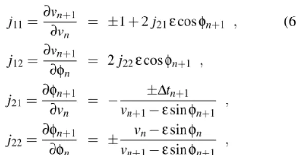
We have then j11=∂vn+1
∂vn
= ±1+2j21εcosφn+1 , (6) j12=
∂vn+1 ∂φn
= 2j22εcosφn+1 ,
j21= ∂φn+1
∂vn
= −v ±∆tn+1
n+1−εsinφn+1
,
j22= ∂φn+1
∂φn
= ±v vn−εsinφn
n+1−εsinφn+1
,
where the plus and minus signs refer to cases 1 and 2, respec-tively.
Thus the map has an invariant measure, namely (v− εsinφ)dv dφ. Ifε=0 the measure is the usual canonical form dE dt.
FIG. 1: Phase space with the rescaled velocity for (a)-(b) the com-plete and (c)-(d) the simplified models. The values of the control pa-rameter are: (a) and (c)ε=1×10⁻³; (b) and (d)ε=1×10⁻⁴. Note that the positions of the first invariant spanning curves are given by
v∗/2√ε≈1.
B. The simplified model (SFUM)
Lieberman and Lichtenberg [2] introduced a simplified ver-sion of the Fermi accelerator. Now, we will suppose that the oscillating wall keeps a fixed positionxW =1 but that, when
the particle suffers a collision with it, the particle exchanges momentum and energy as if the wall were moving. This sim-plification carries the huge advantage of allowing us to speed up our numerical simulations very substantially as compared with those for the full model. It is valid whenvn>>ε. Note
that case 2 of the preceding subsection is impossible and the travel time between two impacts with the “oscillating wall” is simply given by 2/vn, instead of Eq. (5).
Incorporating this simplification into the model, the map can be written as
TS:
( vn+1=
¯ ¯
¯vn−2εsin(φn+1) ¯ ¯ ¯ φn+1=φn+v2n mod 2π
. (7)
The modulus in the equation of the velocity was introduced artificially in order to prevent the particle leaving the region between the walls.
The coefficients of the Jacobian of the simplified map can be derived easily. Now, we have that detJ=±1, implying that the SFUM is area preserving.
C. The phase space
It is well known that the energy in the FUM is bounded [4] because there are invariant spanning curves at sufficiently high energy (velocity). It is also known [2] that the map may have periodic orbits of low energy and thus KAM-like islands may be observed. Figs. 1 (a) and (b), show the typical phase space of the complete model, obtained by numerical iteration of Eq. (4).
The high energy region appears to be very well ordered and the low region seems to exhibit chaotic behavior. Note that there exists a first invariant spanning curve separating two re-gions that have different features: (a) the region above this curve is locally chaotic and structured by the existence of in-variant spanning curves at high energy; and (b) below this curve the region (low energy) is globally chaotic, with KAM islands surrounded by an apparently ergodic sea.
The phase space of the SFUM, obtained by numerical itera-tion of Eq. (7), is shown in Fig. 1 (c) and (d). The structure of its phase space is essentially the same as that of the complete model.
III. SCALING ANALYSIS
A. Rescaling of the phase space
We consider first the SFUM. A naive estimation of the po-sition of the lowest spanning curve may be obtained by trans-forming, locally, the simplified map into the Standard map by means of the coordinate changeIn=v2∗+2v
∗−v n
v∗2 , wherev∗is a typicalvelocity characterizing the region of interest, followed by a linearization around this value. We obtain the Standard map equations
In+1=In−Ke f fsinφn+1 φn+1=φn+In ,
ofKe f f related to the first (lowest) invariant spanning curve.
For eachεthe lowest value ofKe f f corresponds to the
max-imum value of the velocity on the spanning curve, and the highest corresponds to the minimum. Note also thatKe f f has
the same order of magnitude, independent ofε. Moreover, both maximum and minimum values ofKe f fseem to converge
toKc≈0.972 whenεdecreases.
ε (a)Ke f f (b)Ke f f
1×10⁻² 0.77 - 0.94 0.76 - 0.94
5×10⁻³ 0.69 - 0.74 0.69 - 0.76
1×10⁻³ 0.84 - 0.92 0.84 - 0.92
5×10⁻⁴ 0.86 - 0.92 0.86 - 0.92
1×10⁻⁴ 0.95 - 0.97 0.95 - 0.97
5×10⁻⁵ 0.91 - 0.93 0.91 - 0.93
1×10⁻⁵ 0.96 - 0.97 0.96 - 0.97
TABLE I: Characterization of the first invariant spanning curve for the (a) simplified and (b) complete models. Ke f f =4ε/v∗2 is the
effective control parameter. The lowest (highest) value ofKe f f
cor-responds to the maximum (minimum) value of the velocity on the spanning curve.
The position offirstinvariant spanning curve of the FUM can be estimated as before. The values ofKe f f for different
values ofεare also given in Table I. Note that these values are basically the same as the ones obtained for each value ofεof the simplified version.
It seems that the overall characteristics of the phase space are almost independent ofεif the velocities are rescaled by 2√ε, as can be seen in Fig. 1 for both models.
0 1 2 3 4 5
Iteration Number (X108 ) 1.5
1.6 1.8 1.9 2.0
λ
φ0=0
φ0=2π/5
φ0=4π/5
φ0=6π/5
φ0=8π/5
0 1 2 3 4 5
Iteration Number (X108 ) 1.5
1.6 1.8 1.9 2.0
λ
v0=1X10 -3
v0=1X10 -4
v0=1X10 -5
v0=5X10⁻⁴
v0=5X10 -5
V =1X100 -4 φ0=0
FIG. 2: The positive Lyapunov exponent for the low energy region of the SFUM withε=1×10⁻⁴and different initial conditions. It converges to the average valueλ=1.70(2).
B. Lyapunov exponents of the chaotic sea
Let us now characterize the chaotic region below the first spanning curve, for both models. This region still contains
islands with invariant curves surrounding stable periodic or-bits but, outside these islands, we observe an apparently er-godic component. In our numerical simulations, the orbit of any initial condition outside the islands densely fills the same chaotic region. Moreover, as we will see, Lyapunov expo-nents for each of these initial conditions have the same value within the error bars. We will thus evaluate numerically the Lyapunov exponentλassociated with this ergodic component. We choose an initial condition in the chaotic sea. Then, we use the exact form of the tangent mapJ( Eq. (6) for the FUM ) and the triangularization algorithm as proposed in [28] to evaluate
λj= lim N→∞
1 N
N
∑
n=1ln|Λnj| , j=1,2 .
Here,Λn
j are the eigenvalues ofDTN=∏Nn=1Jn, the product
of the Jacobians of the map evaluated along the orbit. We numerically estimate the positive Lyapunov exponent associated with the low energy region bellow the lowest span-ning curve of the simplified model. For each value ofε, we have chosen different initial conditions in the chaotic sea. A typical run is shown in Fig. 2 forε=1×10⁻⁴and 10 different initial conditions. The positive Lyapunov exponent reaches a steady regime for each orbit and all runs seem converge to an average value.
Fig. 3 shows the average value of the positive Lyapunov exponent for different values ofε. Note that the Lyapunov exponent barely seems to depend onε, since it changed only 17% in five decades ofε.
1e-06 1e-05 0.0001 0.001 0.01 0.1
ε
1.38 1.48 1.57 1.68 1.77
λ
FIG. 3: Log-linear plot of the positive Lyapunov exponent as func-tion ofεfor the low energy region of the SFUM.
The same procedure is applied to the FUM. The resulting positive exponents for different values ofεhave a similar be-havior to the SFUM. Indeed, in four decades ofε, the exponent changed also only by 17%. However, for the same value ofε, the positive exponent of the complete model is roughly half the value of the exponent of the simplified model. This dis-crepancy could be related to more refined differences between the models.
The renormalization of the phase space, discussed in the previous subsection, is not only qualitative. The scaling fac-tor is related to the existence of an effective parameterKe f f ∝
thus are well organized and close to being integrable. Low en-ergy regions are associated to largeKe f f and thus associated
with chaos. Well-organized and chaotic regions are present in each phase space, independently ofεup to a size scaling fac-tor. The transition occurs in the first invariant spanning curve when Ke f f ≈Kc≈0.972. Moreover, even though we have
studied a one parameter model which is completely integrable forε=0, one cannot say that it becomes more chaotic by in-creasingεsince the Lyapunov exponent is almost independent ofε.
C. Scaling functions
The results of the previous section suggest that the chaotic sea can be described by rescaled variables. It means that scaling functions are an appropriate framework. Consider ω(n,ε,v0)as a quantity, like velocity or energy, averaged over the initial phase φ0, and depending on the iteration number n, the amplitudeεand the initial velocityv0. The averaged quantity is a generalized homogeneous function [26], if forall valuesof the scaling factorl, the relation
ω(n,ε,v0) =lω(lan,lbε,lcv0) (8) is valid. Here,a,bandcare the scaling dimensions andlan, lbεandlcv0are the so called scaled variables.
First, let us considerv0≈0, a simpler situation in which we have to deal with only two variables. In order to dis-cuss the scaling behavior, we choose l =n−1/a. Then,
we have that ω(n,ε,0) =n−1/aω(1,n−b/aε,0) . The func-tion ω(1,n−b/aε,0) can be written in terms of variablen as ω(1,n−b/aε,0) =g(n/n
x), where the characteristic iteration
numbernxis given by
nx∝ εa/b . (9)
Note that there are two regimes: (a) smalln(n<<nx) and (b)
largen(n>>nx).
In order to describe both regimes, we must know the be-havior ofg(orω(1,n−b/aε,0)) forn<<n
xand forn>>nx.
Consider firstn<<nx. Usually we have thatg≈constant,
implying that ω ∝n−1/a. However the general behavior is g∝n−by/aεy, with the former case being obtained wheny=0.
Therefore, we can write that
ω(n,ε,0)∝n−1+aybεy (10)
forn<<nx.
For largenwe expectωto be idependent ofnand to reach an asymptotic value. If the behavior of g in this regime is g∝n−by′/aεy′, we must have thaty′=−1/b, in order to reach
such asymptotic value. For n>>nx, we therefore have the
following relationship
ω(n,ε,0)∝ ε−1b . (11)
It is less straightforward to discuss the casev06=0. Again choosingl=n−1/a, Eq. (8) can be written as
ω(n,ε,v0) =n−1/aω(1,n−b/aε,n−c/av0) . (12)
Note that we have now two characteristic iteration numbers. For very largen, we expect thatωreaches an asymptotic value independently of the initial velocity, in such way that Eq. (11) remains valid. On the other hand, the behavior for smallncan be very different of that described by Eq. (10).
We can relate the exponentscandbas follows. The initial velocity must be below the first spanning curve, implying that v0,max∼v∗. ButKe f f =4ε/v∗ is a quasi-invariant (Ke f f ≈ Kc≈0.972). We can thus rewrite the effective parameter in
terms of scaled variablesKe f f ∝lb−2c(ε/v0,max),and assume
the invariability (b−2c=0) to obtain thatc=b 2 .
D. The average quantities
We will investigate the evolution of the velocity averaged inMinitial phases, namely
V(n,ε,v0) = 1 M
M
∑
j=1vn,j , (13)
where jrefers to a sample of the ensemble. In this ensemble we can also define the averaged dimensionless energy (E = 2 Energy/mX02w2):
E(n,ε,v0) = 1 M
M
∑
j=1v2n,j . (14)
We are also interested in another kind of average. We first consider the average of velocity and the square veloc-ity over the orbit generated from one initial phaseφ0namely V(n) = 1
n∑ n
i=0vi,andV2(n) = 1n∑ni=0v2i .Then we consider
an ensemble ofMdifferent initial phases:
<V>(n,ε,v0) = 1 M
M
∑
j=1Vj(n) , (15)
<E>(n,ε,v0) = 1
M M
∑
j=1Vj2(n) . (16)
Finally, let us to introduce the roughness, namely
ω(n,ε,v0) = 1 M
M
∑
j=1q
<Vj2>(n)−<Vj>2(n) . (17)
It is worth mentioning that the roughness is an extension of the formalism used to characterize rough surfaces[29].
E. Results for the simplified model
The behavior of the roughness is illustrated in Fig. 4(a) for two values of the parameterε, when the initial velocity is near zero. We can see that it grows for small iteration number nand then saturates at largen. The change between the two regimes is characterized by a crossover iteration numbernx.
100 102 104 106 108
n
10-5 10-4 10-3 10-2 10-1
ω
ε =1 X 10 -4
ε =1 X 10 -3 best fit (a)
100
102
104
106
108
n
10-1 100 101 102
ω/ε
ε =1 X 10 -4
ε =1 X 10 -3 (b)
100
102
104
106
108
n/l2 10-5
10-4 10-3 10-2
ω
/l
ε = 1X10⁻⁴
ε = 1X10⁻³ (c)
FIG. 4: (a) Log-log plot of the roughnessω as a function of the iteration numbern; It is also shown a best fit for shortn. (b) Behav-ior ofω/εas a function ofnin a log-log plot. (c) Collapse of the curves from (a) onto a universal curve. Both curves obtained from the SFUM were derived from an ensemble average of 104different initial phases and always with the same initial velocityv0≈0.
short n. This indicates that the exponent y, defined in Eq. (10), is non-zero. In fact, the transformation ω/εcoalesces the two curves, as shown in Fig. 4(b). Therefore we have that y=1.0(1). Moreover, forε=1×10⁻⁴andn<<n
xa best fit
is shown in Fig. 4 (a) and it furnishes thatω(n,ε,0)∝nβε ,
with the growth exponentβ=0.5000(2). Other fits always furnish values forβaround 0.5. After averaging over different values of the control parameterεin the rangeε∈[10−4,10−1], we then obtainβ=0.496(6). Then, we can conjecture that β=1/2 and relate it to exponentsaandbby Eq. (10). We obtain that−1+b
a =1/2.
From Fig. 4(a), we can also infer : (i) that forn≫nx, the
roughness reaches a saturation regime that is describable as ωsat(ε)∝ εα,whereα is the so called roughening exponent [29]; and (ii) that the crossover iteration numbernxmarking
the approach to saturation isnx(ε,v0)∝ εz ,wherezis called the dynamical exponent.
The exponentαis obtained in the asymptotic limit of large iteration number, and it is independent of the initial velocity. Fig. 5(a) illustrates an attempt to characterize this exponent
0.0001 0.001 0.01 0.1
ε
0.01 0.1
ω
satNumerical Data Best Fit
0.0001 0.001 0.01 0.1
ε
100 1000 10000
n
xNumerical Data Best Fit
a
b
α=0.512(3)
z=-1.01(2)
FIG. 5: (a) Log-log plot ofωsatagainst the control parameterεfor the SFUM. (b) The crossover iteration numbernxas a function ofε
in a log-log plot.
100 102 104 106 108
n
10-4
10-3
10-2
10-1
V
ε=1X10⁻⁴ v0=10
-6
ε=1X10⁻³ v0=10
-6
ε=1X10⁻⁴
v0=10
-3
ε=3X10⁻⁴
v0=3
1/2
X10-3
(a)
100 102 104 106 108
n/l2
10-4
10-3
10-2
V/l
(b)
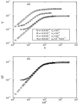
FIG. 6: The average velocityVas a function ofnfor different values ofεandv0in log-log plots. (a) The original iteration number series for the SFUM ; (b) Collapse of the data onto a universal curve for
v0≈0 andv06=0.
using the extrapolated saturation roughness. Extrapolation is required because, even after 103nx iterations, the roughness
has still not quite reached saturation. From a power law fit, we obtainα=0.512(3)≈1/2. Note that this is our worst average value because we have included data for largeε. This best fit value approaches 1/2 as long we consider only small ε. Using Eq. (11) we obtain−1/b=1/2. Since−1+b
a =1/2,
100 102 104 106 108
n
10-8 10-6 10-4 10-2
<E>
ε=1X10⁻⁴
ε=1X10⁻³ best fit (a)
100
102
104
106
108
n
10-2 100 102 104 106
<E>/
ε
2
(b)
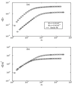
FIG. 7: (a) Behavior of the average energy<E>as a function of the iteration numbernin a log-log plot; It is also shown a best fit for shortn. (b) Behavior of<E> /ε2as a function ofn. Both curves, obtained from the FUM, were averaged first over the orbit and then in an ensemble of 2×10³different initial phases and always with the same initial velocityv0≈0.
scaling dimensions, namelya=2,b=−2 andc=b/2=−1. From Eq. (9), we obtain the dynamical exponentz=a/b=
−1. This exponent can also be found numerically. Fig. 5(b) shows the behavior of the crossover iteration numbernx as
function of the control parameterε. The power law fit gives us thatz=−1.01(2), in good accord with the previous scaling result. Since the fit is clearly worse for large values of the parameterε, we conclude thatz=−1 forεsmall enough.
The scaling forv0≈0 is demonstrated in Fig. 4, where two curves for the roughness in (a) are collapsed onto the univer-sal curve seen in (c) when we normalize the quantities with the exponentsa=2 andb=−2. Note that we have two curves characterized byε1=1×10⁻⁴andε2=1×10⁻³. Using Eq. (8), we obtain the scaling factor l= (ε2/ε1)1/b and the ap-propiate renormalizations of the iteration numbern1=l−an2 and roughnessω1=lω2.
Let us now discuss the scaling whenv06=0. This case is better illustrated by the average velocity (see Fig. 6). Note that there are two characteristic iteration numbers, namely n′x∝1/εandn′′x∝v20/ε2. Since the maximum initial veloc-ity inside the chaotic sea isv0,max≈2ε1/2, the second scale
has a maximum value of (n′′x∼4n′x). So two different kinds of behavior may occur, forn′′x<n′xorn′′x∼n′x. Whenv0=10−6, we haven′′x≈0 and we can see in Fig. 6(a) that the curves for ε=10−4andε=10−3show only two regimes: (i) a growth in power law for n≪n′x and (ii) the saturation regime for n≫n′x. Whenv0=10−3andε=10−4we have thatn′′x<n′x
and we can see for such curve in Fig. 6(a) three regimes: (i) for n≪n′′x, the average velocity is basically constant; (ii) when n′′x<n<n′x, the curve grows and begin to follow the curve of
100 102 104 106 108
n
10-8 10-7 10-6 10-5 10-4 10-3
<E>
ε= 1X10⁻⁴ v0=1X10
-6
ε= 1X10⁻⁴ v0=1X10
-3
ε= 5X10⁻⁴ v0=1X10
-6
ε= 5X10⁻⁴ v0=5
1/2 X10-3
100
102
104
106
108
n/l
10-8 10-7 10-6 10-5 10-4 10-3
<E>/l
FIG. 8: The average energy<E>as a function of the iteration num-bernfor different values ofεandv0in log-log plots. (a) The original iteration number series. (b) Collapse of the data onto universal curves forv0≈0 andv06=0. All curves were obtained from an ensemble of 2×10³initial phases of the FUM.
v0=10−6and sameε; (iii) forn≫n′xwe have the saturation
regime. It is shown in Fig 6(b) that the collapse of the curves holds forv0≈0 andv06=0, implying that the inferred scaling formV(n,ε,v0)with exponentsa=2,b=−2 andc=−1 is also correct.
We have also studied numerically the average energies E(n,ε,v0)and<E>(n,ε,v0). They have a similar scaling behavior. SinceE∼V2, the exponents characterizing the en-ergyα′,β′andy′ can be written in terms of those related to the average velocity and roughness asα′=2α,β′=2βand y′=2y. Then, using Eqs. (10) and (11) it is easy to show that the scaling dimensions of average energies area′=a/2=1, b′=b/2=−1 andc′=c/2=−1/2. These relationships were confirmed numerically.
F. Results for the complete model
The scaling dimensions of the complete model are the same as those obtained for the SFUM. To illustrate this fact, let us discuss the behavior of the energy<E>, first averaged over the orbit and then in the initial phaseφ0.
two values ofεand different initial velocities. Using the ex-ponents just discussed we obtain the collapse shown in Fig. 8(b). Forv0≈0 we can see that after an initial transient the scaling regime is established and the two curves collapse very well onto a universal one. Whenv06=0 we have also the scal-ing behavior. The other quantities (E,ωandV) have similar scaling laws.
Finally, let us summarize our results for the Fermi-Ulam model. We characterized the chaotic region below the first invariant spanning curve (chaotic sea) in the transition from
integrable (ε=0) to non-integrable (ε6=0). All results are valid for small oscillation amplitudeε. The average quanti-ties can be described by scaling functions with characteristic exponents. Since the positive Lyapunov exponent is almost in-dependent ofε, we cannot say that the system becomes more chaotic by increasingε.
J. K. L. da Silva, D. G. Ladeira, E. D. Leonel and S. O. Kamphorst thank to CNPq, CAPES and FAPEMIG, Brazilian agencies, for financial support.
[1] E. Fermi, Phys. Rev.75(6), 1169 (1949).
[2] A. J. Lichtenberg and M. A. Lieberman,Regular and Chaotic Dynamics, Appl. Math. Sci. 38, Springer-Verlag, New York (1992).
[3] M.A. Lieberman and A. J. Lichtenberg, Phys. Rev. A5, 1852 (1971).
[4] R. Douady, Applications du th´eor`eme des tores invariants, Th`ese de 3`eme Cycle, Univ. Paris VII (1982).
[5] L. D. Pustil’nikov, Trudy Moskov. Mat. Obsc.34 (2), 1 (1977); L. D. Pustil’nikov, Theor. Math. Phys. 57, 1035 (1983); L. D. Pustil’nikov, Sov. Math. Dokl. 35(1), 88 (1987); L. D. Pustil’nikov, Russ. Acad. Sci. Sb. Math.82(1), 231 (1995). [6] A. J. Lichtenberg, M.A. Lieberman and R. H. Cohen, Physica
D1, 291 (1980).
[7] E. D. Leonel and P. V. E. McClintock, J. Phys. A38, 823 (2005). [8] P. J. Holmes, J. Soun. Vib.84, 173, (1982).
[9] R. M. Everson, Physica D19, 355, (1986).
[10] E. D. Leonel and P. V. E. McClintock, J. Phys. A 38, L425 (2005).
[11] P. Seba, Phys. Rev. A41, 2306 (1986).
[12] J. V. Jos´e and R. Cordery, Phys. Rev. Lett.56, 290 (1986). [13] S. T. Dembinski, A. J. Makowski and P. Peplowski, Phys. Rev.
Lett.70, 1093 (1993).
[14] S. R. Jain, Phys. Rev. Lett.70, 3553 (1993). [15] G. Karner, J. Stat. Phys.77, 867 (1994).
[16] Z. J. Kowalik, M. Franaszek and P. Pieranski, Phys. Rev. A37,
4016 (1988).
[17] S. Warr, W. Cooke, R. C. Ball and J. M. Huntley, Physica A
231, 551 (1996).
[18] E. Canale, R. Markarian, S. O. Kamphorst and S. P. de Car-valho, Physica D115, 189 (1998).
[19] A. Loskutov and A. B. Ryabov, J. Stat. Phys.108, 995 (2002). [20] E. D. Leonel and P. V. E. McClintock, Chaos 15, 033701
(2005).
[21] J. L. Mateos, Phys. Lett. A256, 113 (1999).
[22] G. A. Luna-Acosta, G. Orellana Rivadeneyra, A. Mendoza-Galv´an and C. Jung, Chaos, Solitons and Fractals 12, 349 (2001).
[23] E. D. Leonel and J. K. L. da Silva, Physica A323, 181 (2003). [24] E. D. Leonel and P. V. E. McClintock, Phys. Rev. E70, 016214
(2004).
[25] E. D. Leonel, J. K. L. da Silva and S. O. Kamphorst, Physica A
331, 435 (2004).
[26] S. Ma, Modern Theory of Critical Phenomena, The Ben-jamin/Cummings Publishing Company, Massachusetts, (1976). [27] E. D. Leonel, P. V. E. McClintock and J. K. L. da Silva, Phys.
Rev. Lett.93, 014101 (2004).
[28] J.-P. Eckmann and D. Ruelle, Rev. Mod. Phys.57, 617 (1985). [29] A. -L. Barab´asi, H. E. Stanley,Fractal Concepts in Surface