THE IMPACT ON CONSUMPTION OF MORE CASH
IN CONDITIONAL CASH TRANSFER PROGRAMS
André Oliveira Ferreira Loureiro* Marcos Costa Holanda†
Abstract
This paper evaluates the impact of an increase in the value of the cash transfer paid to families by the BrazilianBolsa Famíliaprogram. The ex-istence of a similar program in the state of Ceará,Bolsa Cidadão, that in-creases the value received by a sub-group of families, provides a unique dataset, enabling us to evaluate the effect of a higher value of transfer on
the spending of comparable households. There is a significant increase in consumption, but it is smaller than the increment in the income, suggest-ing that the consumption of the households is not properly declared.
Keywords:Poverty; Cash Transfer Programs; Policy Evaluation.
Resumo
O presente artigo avalia o impacto de um aumento no valor do bene-fício do programa Bolsa Família. Isso é possível pela existência no Estado do Ceará de um programa semelhante, Bolsa Cidadão, que na prática au-menta o valor do Bolsa Família para um destas famílias, possibilitando avaliar o efeito de um maior valor de transferência sobre os gastos de fa-mílias comparáveis. É observado um efeito significativo no consumo das famílias. No entanto, a elevação é menor do que o incremento na renda, o que sugere que o consumo das famílias não é corretamente declarado.
Palavras-chave: Pobreza; Programas de Transferência de Renda;
Avalia-ção de Política.
JEL classification:I38, H75, H81.
*PhD Student, Economics, University of Edinburgh. E-mail: [email protected]
†Professor of Economics, Universidade Federal do Ceará. E-mail: [email protected]
1
Introduction
Bolsa Famíliais the largest conditional cash transfer in the world and it is now a consolidated mechanism with favorable evaluations of its impact on poverty in Brazil.1The debate over its validity and effectiveness has been now directed
to its improvement and expansion. A simple but not trivial question emerges from this discussion: Should additional resources be allocated to the program in order to extend its coverage or to increase the value of the benefit?
The Brazilian state of Ceará provides a unique situation to allow us to evaluate the effect of an increase in the value ofBolsa Famíliadue to the
ex-istence of a similar and complementary program called: Bolsa Cidadão. The state government transfers resources to its 41 poorest municipalities in the state, where the poorest families receive a monthly stipend that is added to theBolsa Família. This program allows us to compare families in similar cir-cumstances receivingBolsa Famíliafor different values.
To our knowledge, this is the first attempt to use data of this type to es-timate the effects of higher values of cash transfers on consumption of
com-parable units.2 It is important to highlight that, by performing an evaluation
under these circumstances, some of the most common and difficult problems
to resolve when dealing with matching and impact evaluation are significantly mitigated: self-selection and selection bias.
As in theBolsa Famíliaprogram from the federal government,Bolsa Cidadão
program unifies the actions of all programs of cash transfer existing in the state. It is a benefit that provides an additional amount of cash to the recip-ients of theBolsa Família program, ranging from R$ 5 to R$ 25, which rep-resented, on average, a 20% increase in the Bolsa Famíliabenefit and 7.1% increase in the initial income.3
In order to carry out the proposed evaluation, we use a dataset extracted from the administrative file (Cadastro Único) provided by the Ministry of So-cial Development (Ministério do Desenvolvimento Social — MDS) through the Secretariat of Labor and Social Development of Ceará State (Secretaria do Tra-balho e Desenvolvimento Social), which contains the information of all indi-viduals enrolled in federal and state welfare programs.
In this official database are recorded information upon the family and its
members with monthly per capita income of up to half the Brazilian mini-mum wage.4 Information included in the official database includes
character-istics relative to the household and the individual, such as educational qualifi-cation, profession, income and monthly expenses, among many other relevant variables.
From this dataset we performed an impact evaluation analysis of the fam-ilies that receive both theBolsa FamíliaandBolsa Cidadãobenefits, using the methodology of matching with propensity score, in order to mitigate a likely selection bias in the determination of the recipients of the additional bene-fit. A statistically significant effect on the level of household consumption is
1Some of those papers are Resende & Oliveira (2008), Soares et al. (2009) and Duarte & Sil-veira (2008).
2Filmer & Schady (2010) use a sharp regression discontinuity design to identify the effect of higher values of cash transfers on school attendance in Cambodia.
3The average value received by the families in November 2007 was R$16.00 (About US$9.00). For more detailed figures, see Tables A.2 and A.3 in the Appendix.
found when the income of families who receive the additional cash transfer and families who receive only theBolsa Famíliaare compared. However, the increase in consumption is smaller than the increase in income, suggesting that the consumption of the households is not properly declared.
In the following section, the program coverage is defined, as well as the sample used in the analysis. In section 3, the methodology used is described, while section 4 discusses the effects of participation in the program on
con-sumption. The fifth section concludes.
2
Sample Delimitation, Program Coverage and Descriptive
Statistics
2.1 Sample Delimitation
In the Cadastro Únicodatabase for the state of Ceará, there were more than 5 million and 800 thousand individuals in November 2007. In order to en-able more consistent and relien-able estimates, the dataset were constrained to the entries updated between January and November 2007, in order to avoid distortions, especially in monetary variables.5
When we also constrain the database only to people living in the 41 poor-est municipalities where the Bolsa Cidadãowas provided, the sample size is reduced to 695.027 people, which represents 78% of the total population of those municipalities.
Table A.1 in the Appendix shows the rates of inclusion inCadastro Único
database, as well as participation inBolsa FamíliaandBolsa Cidadãoby munic-ipality. The percentage of the total population in the official database is very
high. This is partially explained by the fact that those municipalities are the ones with the highest social vulnerability in the state.6
2.2 Program Coverage
The percentage of coverage of theBolsa Famíliais quite high, with most of the municipalities with more than 80% of registered people receiving the bene-fit. For theBolsa Cidadãoprogram, the percentage of coverage is not quite as high, just over 15% in the 41 municipalities with recipients of this additional benefit.
Table 1 presents the coverage ofBolsa CidadãoandBolsa Famíliaprograms in municipalities taking into account two criteria. The coverage with respect to the total population of the municipality and coverage with respect to the population registered in theCadastro Únicodatabase. It is worth noting that there is not a large reduction in the coverage of both programs when consid-ering the total population of the municipality as a reference instead of the
5Another advantage of this approach is to improve the quality of information. As highlights Loureiro (2007), theCadastro ÚnicoDatabasehas some difficulties that were progressively miti-gated by MDS.
population registered in theCadastro Únicodatabase. This indicates the high level of poverty in these locations.
Table 1: Bolsa Família and Bolsa Cidadão Coverage in the 41
municipali-ties
Bolsa Família Bolsa Cidadão
Total Population 890,926 890,926
People in Cadastro Único database 695,027 695,027 Population not receiving the benefit 133,580 585,219 Population receiving the benefit 561,447 109,808
Program Coverage (Total Population) 63.02% 12.33% Program Coverage (Cadastro Único database) 80.78% 15.80%
Note: Information in November — 2007. Data Source: Cadunico/MDS.
2.3 Descriptive Statistics
Aiming a better understanding of the characteristics of people included in the database in the 41 municipalities which have benefited families with theBolsa Cidadãoprogram, some descriptive statistics concerning the households, such as educational level, school attendance and condition in the labor market are presented below. The following statistics are related to all families registered in the database, regardless of whether or not they are receiving the benefits. Table 2 below shows the school attendance of people between 7 and 17 years of age who were registered in the municipalities under analysis. It can easily be noticed that the percentage of people in this age group who is not attending school is just over 11%. Furthermore, it is interesting to note that over 87% of the students are enrolled in public schools, with the great majority of the pupils attending schools under municipal administration. It is worth noting that less than 1% of them are enrolled in private schools.
Table 2: School Attendance of the
population in the database between 7 e 17 years of age
School Attendance % Municipal Public 81.50
State Public 5.69
Federal Public 0.01
Private 0.62
Other 0.15
Not enrolled at school 11.53
N/A 0.49
Total 100.00
Note: Information in November — 2007. Data Source: Cadunico/MDS.
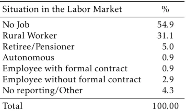
than 54% of the population between 15 and 65 years of age that are registered inCadastro Únicodatabase do not work. The second most frequent category is that of rural workers, followed by to retirees and pensioners. It is also notable the participation of people with formal employment, which reaches less than 1% of people registered in the database.
Table 3: Situation in the Labor Market of the
population in the database in working age
Situation in the Labor Market %
No Job 54.9
Rural Worker 31.1 Retiree/Pensioner 5.0 Autonomous 0.9 Employee with formal contract 0.9 Employee without formal contract 2.9 No reporting/Other 4.3
Total 100.00
Information in November — 2007. Data Source: Cadunico/MDS.
Another important aspect regards the source of income (excluding bene-fits) of households. Table 4 displays the share of each source of income among the people included inCadastro Únicodatabase, which shows that almost 50% of people that have a source of income obtain it from labor. Note also that re-tirement and pensions benefits are the other main sources of income.
Table 4: Sources of Income of
households in the database
Sources of Income % Labor 49.8
Retirement/Pension 32.7
Unemployment Benefit 0.1
Alimony 0.6
Other Income 16.8
Total 100.00
Information in November — 2007. Data Source: Cadunico/MDS.
Table 5: Destination of the Expenditures of households in the database
Destination of the Expenditures %
Food 64.2
Rent 2.1
Housing Financing 0.2
Water 2.3
Electricity 6.5
Transport 2.7
Medicines 6.9
Cooking Gas 10.1
Other Expenditures 5.0
Total 100.00
Information in November — 2007. Data Source: Cadunico/MDS.
3
Empirical Framework
In order to assess the impact of a family receiving an additional direct income transfer, we restricted the sample only to families that areBolsa Família recipi-ents.7 Because this is also a condition for a family to receive theBolsa Cidadão
benefit, this procedure does not eliminate any of those families from the sam-ple. This procedure also significantly mitigates the problem ofselection bias.8
However, even after that, it is still possible (in fact likely) that a family will participate in theBolsa Cidadão program if it has some specific charac-teristics. In order to mitigate this problem we will use matching based on propensity score in order to estimate the causal effects of the treatment. In
the present study, this method will be employed to evaluate the effects of the Bolsa Cidadãobenefit on expenditures of beneficiary families which comprise consumption in items such as food, housing, clothing, education and other expenses.
This impact is identified in the literature of impact assessment as Average Treatment Effect (ATE). This concept emerges from a framework based on
the idea of counterfactual, where the impact of a treatment is evaluated by comparing the effect of the treatment on an outcome variable between two
situations: the situation of an individual with the treatment and status of that same individual, if he had not received treatment.9
Denoting the consumption of the families with the additional benefit byY1
andY0the consumption of families without treatment, it is clear that a family
cannot be in both situations simultaneously. To measure the treatment effect,
we should look for the difference between results with and without treatment, Y1−Y0. Note that this difference remains a random variable. Considering the
7It is not unusual the situation in which there is more than one family in a given household. In this paper, we use the two words interchangeably to denote the entity with a common head.
8This session is based on Wooldridge (2002, chap. 18) and Lee (2005). For a recent survey on the propensity score matching literature, see Caliendo & Kopeinig (2008).
average difference between the families under analysis, which may include a
set of covariates as controls (x), we have the average treatment effect:
AT E=E(Y1−Y0|x) (1)
ATE is the expected effect of treatment on a family selected at random from
a population. A more common alternative measure in the literature would be the average treatment effect in the treated (ATT), that is, for those who actually
participated in the program (w= 1, otherwise,w= 0). It is often denoted by:
AT T =E(Y1−Y0|w= 1, x) (2)
One must bear in mind that those procedures are only valid under random-ization and some other assumptions.10 In this case, a simple statistical test of
comparison of averages would be sufficient. However, as in the great majority
of the situations in social sciences, a randomized sample is not only difficult
to carry out, but very unlikely to be accepted by the candidate recipients or policy makers.
In the present case, programs such asBolsa FamíliaandBolsa Cidadãouse some specific eligibility criteria so that there is a selection bias if outcomes between recipients and non-recipients are considered. Moreover, what also usually happens is the phenomenon known as self-selection into treatment. That is, individuals determine, at least partially, if they will receive treatment. Nevertheless, because the criteria used are the same, and everyBolsa Cidadão
recipient is also a Bolsa Famíliarecipient, most of these issues are resolved when a comparison between these two groups is carried out.
However, it is still possible to argue that even in the case of comparable households, some selection bias will emerge in the process of determination of the additional benefit. In order to mitigate this problem, the propensity score methodology is implemented.
3.1 Selection on Observable Variables: The Propensity Score
As mentioned earlier, in the case where participation is not drawn randomly, a simple comparison between families participating and not participating in the program could lead to misleading conclusions, due to, at least, two rea-sons. First, ex-post differences of the results could simply reflect differences
that existed before the program. Second, the effect of the program may be a
function of background variables (education of the head of the family, number of children, etc.) that may differ between treatment and control groups. These
problems can be mitigated by using the method of matching with propensity score.11
To deal with the problem of pairing, Rosenbaum & Rubin (1983) devel-oped a method known as propensity score matching. These authors showed that the matching procedure can be implemented through a single control variable, the propensity score. The propensity scorep(x) is defined as the
con-ditional probability of a family receiving the treatment given their observable characteristicsx. That is,p(x) =Prob(w= 1|x).
10In the case of a randomized experiment ATE and ATT are equal. For further detail, see Wooldridge (2002, chap. 18) and Lee (2005).
Rosenbaum & Rubin (1983) show that in equation 2,xcan be replaced by
p(x), thus:
E(Y1−Y0|w= 1, p(x)) =E(Y1|w= 1, p(x))−E(Y0|w= 0, p(x)) (3)
If the treatment and outcomes are independent conditional on pre-treat-ment variables, these are also independent conditional on the probability of receiving treatment given to observable characteristics, i.e., conditional on propensity score.12
(Y0, Y1⊥w|p(x)) (4)
However, as Rosenbaum (2002) points out, the propensity score methodol-ogy solves only two of the three likely sources of bias in the estimation of the ATT, the common support bias and the overt bias (generated by observed fac-tors). A third source of bias, the covert bias (generated by unobserved factors), may be reduced by this procedure, but not completely eliminated. As it will be discussed, there are some reasons to believe that the bias stems basically from observable factors.
3.2 Unobserved Heterogeneity: Covert Selection Bias
When we consider the existence of unobserved factors (u) influencing the probability of being aBolsa Cidadãorecipient and we explicitly consider those variables to each familyi, the propensity score can now be denoted by:
pi=p(xi, ui) =Prob(wi= 1|xi, ui) (5)
That implies that two families with exactly the same values for the co-variates x can have different probabilities of receiving the treatment. That
would be the case if, for example, families were more likely to receive the addi-tional benefit if they knew someone working in the municipal administration. Rosenbaum (2002) showed that the ATT only maintain its causal interpreta-tion if unobserved factors caused the relative likelihood of treatment to differ
between treatment and control groups with similar observed characteristics by a quantity within reasonably high bounds.13 The analysis is performed by
expressing the treatment propensity in terms of odds. In the present case, the odds of treatment are given by pi
1−pi and inform the relative likelihood that a
family will receive the additional benefit. For two familiesiandj, the ratio of
their odds is given by
pi
1−pi
pj
1−pj
=pi
1−pj
pj
1−pj
(6)
In the present case, the odds ratio reflects the relative and ex ante likeli-hood of treatment for an actually treated individual relative to an untreated
12Another important assumption iscommon support, that is, for any givenx, both treated and control individuals have propensity scores within the (0,1) interval.
individual. If the probability of treatment is assumed to follow a logistic14 distribution, expressed in terms of its cumulative distribution function
pi =F(βxi+γui) =
1
1 +e−(βxi+γui) (7)
whereβandγare vectors of coefficients that capture respectively the
sensitiv-ity of the probabilsensitiv-ity of treatment to observed and unobserved factors. Using equation 7 into equation 6 and rearranging leads to:
eβxi+γui
eβxj+γuj (8)
For a pair of two matched families i and j that consequently share the
same vector of observable covariates, the odds ratio is a quantity independent ofx:
pi
1−pi
pj
1−pj
=eγ(ui−uj) (9)
The odds ratio is different from one unless the unobservable factors are
negligible to determine the probability of treatment (γ= 0) and/or the unob-served values for both matched individuals are identical (ui =uj), in which
case there is no hidden or covert selection bias. For example, if the odds ratio is greater than one, a treated individual was, ex ante, more likely to receive the treatment relative to an untreated individual even after controlling for the observable characteristics.
We follow the literature and assume that the unobserved factor is a di-chotomous variable: ui ∈ {0,1} and denoteeγ =Γ. Rosenbaum derived the
following bounds for the odds ratio:
1
Γ≤
pi
1−pi
pj
1−pj
≤Γ (10)
IfΓ= 1, two matched families (one treated and one untreated) with similar
propensity scores have the same probability of receiving the additional benefit and there is no covert bias. IfΓ= 2, even though two matched families share
similar observable characteristics, the family with the extra benefit was ex ante 2 times more likely to receive the treatment when compared to a similar family that did not receive the benefit.
If the difference between treated and untreated families is statistically
sig-nificant, even for low values ofΓ, the hypothesis of covert bias affecting the
re-sults cannot be rejected. Nevertheless, it must be emphasized that the Rosen-baum bounds represent a worst case scenario.
3.3 Calculating the ATT
There are several alternatives of matching methods to calculate the average treatment on the treated (ATT), established in the program evaluation
ture.15 We will focus on four methods of calculating the ATT: Nearest Neigh-bour, Radius (Nearest Neighbour with more than one neighbor), Stratification and Kernel.
The method of pairing the nearest neighbor, as the name suggests, selects the non-treated individuals to be compared to a treated one when they have the propensity score closest to each other. We follow the notation adopted in the impact evaluation literature and defineT to be the set of treated units andCthe set of control units, andYT andYCthe results of those treated and control, respectively. DenotingC(i) as the set of control individuals matched with the treated individuali with an estimated propensity corepi. Thus, we
have:
C(i) =minkpi−pjk, i,j (11)
It is worth noting thatC(i) is a singleton set unless there are multiple
near-est neighbors. The Radius near-estimator allows all individualsjwithin a certain
radiusrto be controls for a treated individuali:
C(i) =npj| kpi−pjk< r, i,j
o
(12)
The ATT estimator for both cases above is given by:
AT TN N=AT TR= 1
NT X
i∈T
YiT− X
j∈C(i)
wijYjC , (13)
with the correspondingC(i) for each estimator andwij=N1C i
ifj∈C(i), wij= 0
otherwise.
The method of stratified matching is performed by dividing the variation in the propensity scores into intervals such that each of treated and control units have on average the same propensity score. Then, in each interval, the difference in average scores between groups of participants and
nonpartici-pants is calculated. The ATT is finally obtained by the weighted average of these differences, with the weights being determined by the distribution of
units between the treated blocks. In the stratified matching method, the ob-servations in the blocks that have no treatment or control are discarded. Defin-ingqas the index of the blocks defined in the range of propensity score within
each block is computed, we have:
AT TqS= P
i∈I(q)YiT
NTq − P
j∈I(q)YTi
NqC
(14)
whereI(q) represents all the units in blockq, whileNT
q andNqCrepresent the
amounts of treated and control units in blockq, respectively.
The Kernel matching estimator assigns weights on each controls decreas-ing on the distance (in terms of the propensity score) to the treated individual:
AT TK= 1
NT X
i∈T
YiT−
P
j∈CYCj G
pj−pi
h
P
k∈CG
pk−pi
h (15)
whereG(·) is a kernel function and h is the bandwidth. It can be interpreted as a particular version of the Radius method.
4
Program Participation and e
ff
ects on Consumption
4.1 Additional Sample Delimitation
In the estimation of the propensity score, we need to define some variables that are likely to explain the participation in theBolsa Cidadãoprogram. How-ever, as the following analysis will show, many relevant variables would be re-dundant, if we considered the whole sample (all individuals in all households). In order to avoid this problem, all information from the families was grouped, so that all individuals of one family have information that are common and linked to each member of the family. Therefore, only the heads of each family are kept in the data, and although information from the households is main-tained, the problem of redundant information is overcome. Additionally, all observations with inconsistent levels of income and consumption were dis-carded.
4.2 Descriptive Statistics
Table 6 below shows the descriptive statistics for consumption per capita and the variables used in the estimation of the propensity score. The 57,523 obser-vations refer to families in 41 municipalities covered by both programs. The variables of personal attributes such as age, race and sex refer to the head of the family. The first seven variables are continuous while the others are bi-nary, taking 1 when they have the attribute in consideration and 0 otherwise. Since they are dichotomous variables, the average of these variables informs the proportion of the population in question that have the attributes. Still from Table 6, one can see that 11,556 households receive the additional bene-fit, which represents over 20% of households in the data.16
The households with the additional conditional cash transfer have a sta-tistically significant higher level of consumption, even though the average income is not statistically different. However, this 4.78% higher consumption
might be affected by observable variables. One of these variables seems to be
the amount received from theBolsa Famíliaprogram in per capita terms. The amount paid for households with the Bolsa Cidadãoprogram is significantly smaller than the per capita value received by families without the additional benefit.
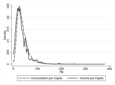
Some other relevant conclusions may be taken from Table 6. More than 96% of the household heads are women. Besides, the average consumption per capita level is almost R$ 4 higher than the average income per capita, indicating, in general a certain degree of indebtedness.17
Figure 1 depicts the distribution of income and consumption per capita, letting clear the high degree of inequality among the poor and that almost the whole of both distributions are below R$ 100 per month per capita. Another relevant characteristic is the fact the consumption distribution is considerably
16Note that the difference between this number and presented in section 2 is due to the restric-tions made in the sample.
Lo
ur
eir
o
an
d
H
ola
nd
a
E
co
no
m
ia
A
pli
ca
da
,v
.1
7,
n.4
Table 6: Descriptive Statistics
Variable Bolsa Cidadão
andBolsa Família
Recipients Bolsa Família only
Mean S. Dev. Min Max Mean S. Dev. Min Max Consumption per Capita 39.07 23.19 1.43 258 37.25 23.11 1.01 286 Income per Capita 34.68 28.97 0 380 34.69 27.30 0 380
Bolsa Famíliaper capita 21.67 8.84 1.8 76 22.02 9.38 1.64 116 Age 37.22 10.90 17 94 37.48 11.07 16 92
Number of People in HH 4.30 1.78 1 15 4.26 1.77 1 16
Number of Rooms in HH 4.71 1.64 1 16 4.66 1.61 1 19
Male 0.03 0.17 0 1 0.04 0.19 0 1
Non-white 0.77 0.42 0 1 0.74 0.44 0 1
Married 0.73 0.44 0 1 0.72 0.45 0 1
Unemployed 0.31 0.46 0 1 0.34 0.47 0 1
Elementary School 0.15 0.36 0 1 0.15 0.36 0 1
High School 0.07 0.26 0 1 0.08 0.26 0 1 Urban 0.35 0.48 0 1 0.35 0.48 0 1 Brick Household 0.76 0.43 0 1 0.77 0.42 0 1 Appropriate Sewer 0.25 0.43 0 1 0.25 0.44 0 1 Crop Insurance Recipient 0.13 0.34 0 1 0.11 0.31 0 1 Number of Observations 11,556 45,967
0
.005
.01
.015
.02
.025
Density
0 100 200 300 400
R$
Consumption per Capita Income per Capita
Data Source: Cadunico/MDS.
Figure 1: Distribution of Consumption and Income per capita
smoother than the income distribution, revealing a greater inconsistence in the declaration of the monthly amount of income.
4.3 Propensity Score Estimation
As discussed above, even with the comparison of two extremely similar groups, it is still possible that there is selection bias. In order to mitigate this problem, the propensity score model is estimated and presented in Table 7. The specifi-cation of the model that determines the likelihood of receiving the additional benefit was obtained, as usual, by observing the balancing property for all co-variates. The use of a less parsimonious model is justified by the fact that the greater the number of variables included, the better the matching performed, since the higher the number of observable characteristics used, the more sim-ilar are the individuals in the treatment and control groups.18
In the estimated model, most control variables are statistically significant and have the expected effects, what suggests that the included factors are
rele-vant to determine treatment. It is observed that the number of children in the household increases the likelihood of participation in theBolsa Cidadão pro-gram. The fact that the head of household is unemployed, male or white de-creases this probability. Married individuals, located in urban areas, in house-holds with greater numbers of rooms are more likely to be eligible for the program. In addition, households made of brick are less likely to be selected, while families who participate in the Crop Insurance program are more likely to receive theBolsa Cidadãobenefit.
Table 7: Propensity Score Estimation —Bolsa CidadãoRecipient
Coeff. Std. Error t-test p-value
Constant −1.7292 0.2602 −6.65 0.000 Male −0.5065 0.1435 −3.53 0.000 Non-white 0.0047 0.0599 0.08 0.938 Age 0.0666 0.0124 5.35 0.000 Age2 −0.0019 0.0003 −6.50 0.000
Married 0.1452 0.0154 9.41 0.000 Income in the HH per Capita −0.0052 0.0013 −3.90 0.000
Bolsa Famíliaper capita −0.0001 0.0010 −0.06 0.951 Unemployed −0.1174 0.0137 −8.58 0.000 Elementary School 0.0366 0.0241 1.52 0.128 High School −0.0549 0.0318 −1.73 0.084
Number of People in the HH 0.0021 0.0038 0.57 0.570
Number of Rooms 0.0054 0.0331 0.16 0.869
Urban 0.0253 0.0139 1.83 0.067
Brick Household −0.1135 0.0723 −1.57 0.116
Appropriate Sewer in the HH −0.0744 0.0636 −1.17 0.243
Crop Insurance Recipient −0.0172 0.0278 −0.62 0.535
Data Source: Cadunico/MDS.
Figure 2 shows the nonparametric distribution of the propensity score comparing control and treatment groups. Interestingly, the distribution for treated and control groups do not differ significantly, as one might expect.
This is likely due to the fact that we are only consideringBolsa Família recipi-ents, what makes most households in our sample very homogeneous. Yet, we could expect significant differences if the supplementary program had
prior-itized a specific group of families. This evidence strongly suggests that the choice of theBolsa Cidadãorecipients was reasonably random among the fam-ilies participating in theBolsa Famíliaprogram.
4.4 Estimation of Impact of a higher value ofBolsa Família on Consumption
Table 8 shows the estimates of the impact of Bolsa Cidadão benefit on the consumption per capita for the 41 non-contiguous municipalities using the estimated propensity score and the four matching methods described in the previous section: nearest neighbor, radius, stratification and kernel matching, with the nearest neighbor estimates being reported for 1 and 2 neighbours. In general, it is possible to identify a positive and statistically significant effect
on consumption, if the family receives the additional cash transfer, which is around R$ 2.00 per month.19
The first part of the table displays the results of estimating the average treatment effect on the treated using matching by stratification method. To
match the 11,556 families that received the additional benefit were generated 45,966 control families, with an ATT of 2.235.
0
2
4
6
8
kdensity
_pscore
0 .2 .4 .6 .8
x
Treated Control
Data Source: Cadunico/MDS.
Figure 2: Propensity Score: Treated vs Control
In order to test the robustness of this result, the ATT was estimated by the method of matching of nearest neighbor with one and two neighbors. Like the stratification method estimate, the impact of the additional cash transfer in the estimates based on the nearest neighbor method is positive, significant and around R$ 2.00.20
Table 8: ATT Estimate: Nearest Neighbor, Radius, Stratification and
Kernel Matching
Matching
Method Number ofTreated Number ofControls ATT StandardError t-test Covert BiasBounds (Γ)
Stratification 11,556 45,966 2.235 0.225 9.95 1.10−1.15 Nearest Neighbor
(One neighbor) 11,556 45,966 2.194 0.345 6.35 1.15
−1.20
Nearest Neighbor (Two neighbors)
11,556 45,966 1.966 0.294 6.67 1.03−1.04
Radius 11,352 44,516 2.239 0.248 9.02 1.02−1.03 (caliper=0.0001)
Kernel 11,556 45,958 1.739 0.245 7.09 1.02−1.03 Note: The number of treated and controls refers to the effectively matched by the corresponding matching method. Bootstrapped standard errors.
Data Source: Cadunico/MDS.
The last two matching methods are the radius and kernel, generating ATTs of 2.239 and 1.739, respectively. Note that because of the restriction in the size of the radius, the number of treated and controls in the radius method were 11,352 and 44,516, respectively.
The increase in consumption varies from 4.67% (kernel) to 6.01% (strat-ification) when compared with the households that receive only the Bolsa Famíliabenefit. Except for the kernel estimate, these figures are marginally higher than the 4.78% observed by the mean comparison, which would corrob-orate with the fact that poorer households are selected to the additional pro-gram. These numbers are also consistent with the fact that theBolsa Cidadão
program represents an income increase of 7.12% in the household per capita income.
Nevertheless, the narrow gap between the estimated ATTs and the diff
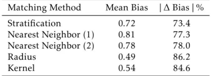
er-ence between the treated and control before matching casts some doubt on the assumption that there was a selection to receive theBolsa Cidadãobenefit, based on observed characteristics of the families, like the level of income. This is despite the fact that there was considerable bias reduction after matching for all matching methods used, presented in Table A.1 in the appendix. The reduction in the mean absolute standardized bias between the matched and unmatched families varies between 73.4 and 86.2.
In order to consider the importance of the influence of unobserved factors, Table 8 also presents the sensibility of the results to the presence of covert bias, displaying the critical levels of Γ described in section 3.2. The small
values indicate that unobserved factors, such as the fact that a family knows someone in the municipal administration, can play an important role in the results. Covert bias is a likely possibility as the critical levels ofΓin which the
conclusion of an effect of the additional benefit is as little as 2% in the case
of the radius and kernel matching methods and 20% in the nearest neighbor with one control for each treated unit.
Nevertheless, it must be taken into account that such sensitivity analysis represents a worst case scenario. DiPrete & Gangl (2004) emphasize that even in the cases in which the critical levels ofΓare very small, the ATT estimates
would be inconsistent only if unobserved factors caused the odds ratio of treat-ment to differ between treatment and control groups by a small factor and
if the effects of those confounding factors on the outcome variable were
ex-tremely strong. In the present case, if the confounding factors had a relevant effect on the likelihood of receiving the additional benefit but little influence
on consumption levels, the ATT estimates would still be consistent.
5
Conclusion
This paper presents an analysis of the impact of an increase in the Bolsa Famíliaprogram on the consumption of households by using a unique data set in Brazil. This was possible by comparing households that are recipients of bothBolsa FamíliaandBolsa Cidadãoprograms with households that receive only the former.
Nevertheless, a sensitivity analysis pointed out the possibility that unob-served factors could be driving the results. Moreover, as the marginal propen-sity to consume is assumed to be closer to one when we consider lower quan-tiles, one might expect a higher increase in the consumption. This could be re-lated to a measurement error in the consumption basket referenced in Cadas-tro Únicodatabase, since the information is self-reported. This misreporting could be largely related to the fact that part of the extra resources generates an income effect that boosts the purchase of durable goods, which are
gen-erally paid in monthly installments, which people tend not to recognize as consumption.
Acknowledgements
The authors thank the Secretariat of Labor and Social Development of Ceará State (Secretaria do Trabalho e Desenvolvimento Social do Ceara) and Caixa Econômica Federal for proving the data used in this paper. André Loureiro also would like to gratefully acknowledge the support from Fundação Cearense de Apoio ao Desenvolvimento Científico e Tecnológico — FUNCAP.
Bibliography
Aakvik, A. (2001), ‘Bounding a matching estimator: the case of a norwegian training program’,Oxford bulletin of economics and statistics63(1), 115–143.
Angrist, J. D., Imbens, G. W. & Donald, B. R. (1996), ‘Identification of causal effects using instrumental variables’,Journal of the American Statistical Asso-ciation91(434), 444–455.
Attanasio, O., Meghir, C. & Vera-Hernandez, M. (2004), Baseline report on the evaluation of familias en accion, Open access publications from univer-sity college london, Univeruniver-sity College London.
Becker, S. & Caliendo, M. (2007), ‘Mhbounds-sensitivity analysis for average treatment effects’,Stata Journal7(1), 71–83.
Becker, S. O. & Ichino, A. (2002), ‘Estimation of average treatment effects
based on propensity scores’,Stata Journal2(4), 358–377.
Caliendo, M. & Kopeinig, S. (2008), ‘Some practical guidance for the im-plementation of propensity score matching’, Journal of economic surveys 22(1), 31–72.
DiPrete, T. A. & Gangl, M. (2004), ‘Assessing bias in the estimation of causal effects: Rosenbaum bounds on matching estimators and
instrumen-tal variables estimation with imperfect instruments’,Sociological methodology 34(1), 271–310.
Filmer, D. & Schady, N. (2010), ‘Does more cash in conditional cash transfer programs always lead to larger impacts on school attendance?’, Journal of Development Economics.
Heckman, J. J. (1991), Randomization and social policy evaluation, NBER Technical Working Papers 107, National Bureau of Economic Research, Inc.
Heckman, J. J., Ichimura, H. & Todd, P. E. (1997), ‘Matching as an econo-metric evaluation estimator: Evidence from evaluating a job training pro-gramme’,Review of Economic Studies64(4), 605–54.
Imbens, G. W. & Angrist, J. D. (1994), ‘Identification and estimation of local average treatment effects’,Econometrica62(2), 467–75.
Lee, M.-J. (2005),Micro-Econometrics for Policy, Program, and Treatment Ef-fects, Advanced Texts in Econometrics, Oxford University Press.
Loureiro, A. O. F. (2007), Uma analise da pobreza no ceara a partir dos dados do cadunico, Nota Tecnica - IPECE 27, IPECE.
Resende, A. & Oliveira, A. M. (2008), ‘Avaliando resultados de um programa de transferencia de renda: O impacto do bolsa-escola sobre os gastos das familias brasileiras’,Estudos Economicos38(2), 235–265.
Rosenbaum, P. R. (2002),Observational studies, Springer.
Rosenbaum, P. R. & Rubin, D. B. (1983), ‘The central role of the propensity score in observational studies for causal effects’,Biometrika70(1), 41–55.
Rubin, D. B. (1974), ‘Estimating causal effects of treatments in randomized
and nonrandomized studies’, Journal of Educational Psychology66(5), 688– 701.
Soares, S. S. D., Ribas, R. P. & Soares, F. (2009), Focalizacao e cobertura do programa bolsa-família: Qual o significado dos 11 milhoes de familias?, Dis-cussion Papers 1396, Instituto de Pesquisa Economica Aplicada - IPEA.
Appendix A
Table A.1: Situation in the Labor Market of the
population in the database in working age
Matching Method Mean Bias |∆Bias|%
Stratification 0.72 73.4
Nearest Neighbor (1) 0.81 77.3
Nearest Neighbor (2) 0.78 78.0
Radius 0.49 86.2
Kernel 0.54 84.6
Table A.2: Values and percentages of the benefits: Bolsa CidadãoX Bolsa Família
Bolsa Cidadão
0 5 10 15 20 25 Total %
BF
0 558664 145 445 270 105 58 559687 0.808 18 4234 556 237 344 75 12 5458 0.008
23 1 - - - 1 0
26 115 77 11 3 1 - 207 0
36 2670 82 361 123 173 43 3452 0.005
38 1 - - - 1 0
41 6 - 6 - - 1 13 0
44 29 - 21 4 - 1 55 0
51 2 - - - 2 0
54 1279 11 23 153 38 118 1622 0.002 58 18472 29 3464 640 56 7 22668 0.033
59 3 - - 2 - - 5 0
61 5 - - - 5 0
62 7 - - 3 - - 10 0
64 1 - - - 1 0
66 34 - - 1 - - 35 0
72 2 - - 1 - - 3 0
76 29421 524 1113 4432 732 76 36298 0.052
77 2 - - - 2 0
79 1 - - 1 - - 2 0
81 3 - - - 1 - 4 0
84 287 7 2 122 22 2 442 0.001
91 2 - - - 1 - 3 0
94 25382 18 533 1346 2569 574 30586 0.044
96 1 - - - 1 0
97 2 - - - 2 0
99 44 - - - 9 1 54 0
102 155 - 2 - 54 9 220 0
108 4 - - - 4 0
112 24943 48 180 518 759 4481 30929 0.045
114 7 - - - - 1 8 0
115 4 - - - 4 0
116 22 - 3 - 1 - 26 0
117 29 - - - - 6 35 0
119 1 - - - 1 0
120 206 - - - - 112 318 0
127 2 - - - 2 0
134 3 - 1 1 - - 5 0
135 123 - - - - 35 158 0
142 1 - - - 1 0
150 41 - - - - 12 53 0
152 16 - - - 16 0
155 2 - - - 2 0
165 7 - - - 7 0
166 - - - 1 - - 1 0
188 18 - - - 1 - 19 0
224 14 - - - 14 0
240 1 - - - 1 0
Table A.3: Municipalities with Bolsa Cidadãorecipients and participa-tion in the programs
Municipality Total Popu-lation
Cadastro
Único % BolsaFamília % BolsaCidadão % Aiuaba 15500 11471 0.74 9877 0.861 677 0.059 Alcantaras 10349 7950 0.768 6522 0.82 1932 0.243 Apuiares 15111 8675 0.574 8063 0.929 523 0.06 Araripe 21474 21755 1.013 14585 0.67 4191 0.193 Arneiroz 7666 5785 0.755 4819 0.833 1110 0.192 Assare 21964 18062 0.822 13960 0.773 1432 0.079 Aurora 25816 19318 0.748 16654 0.862 1532 0.079 Barroquinha 14765 12515 0.848 9915 0.792 4138 0.331 Boa Viagem 52337 41158 0.786 33582 0.816 5074 0.123 Carire 19357 13540 0.699 11981 0.885 557 0.041 Caririacu 29487 23330 0.791 19130 0.82 7716 0.331 Carius 19186 15190 0.792 12756 0.84 1522 0.1 Catarina 18619 8133 0.437 7219 0.888 1846 0.227 Chaval 13526 10513 0.777 8407 0.8 849 0.081 Coreau 22035 16107 0.731 14116 0.876 1648 0.102 Farias Brito 22602 17199 0.761 13211 0.768 1709 0.099 Graca 15194 12316 0.811 10491 0.852 2011 0.163 Granja 54422 37826 0.695 32057 0.847 7740 0.205 Hidrolandia 17506 14570 0.832 12493 0.857 1073 0.074 Iraucuba 21605 18138 0.84 14704 0.811 6254 0.345 Itatira 16976 17596 1.036 12491 0.71 6632 0.377 Jardim 28497 21666 0.76 17814 0.822 972 0.045 Madalena 16738 14200 0.848 9853 0.694 1014 0.071 Massape 34578 26346 0.762 19532 0.741 2613 0.099 Miraima 12578 9462 0.752 7804 0.825 798 0.084 Mombaca 41540 33118 0.797 26784 0.809 1400 0.042 Moraujo 7704 6199 0.805 5266 0.849 1232 0.199 Morrinhos 20821 12978 0.623 11633 0.896 713 0.055 Mucambo 15392 11066 0.719 9033 0.816 902 0.082 Ocara 23077 17608 0.763 15076 0.856 6413 0.364 Parambu 34192 27918 0.816 22163 0.794 5860 0.21 Potengi 9980 6988 0.7 5761 0.824 1536 0.22 Quiterianopolis 19214 16414 0.854 13198 0.804 5283 0.322 Reriutaba 24557 15057 0.613 12556 0.834 1416 0.094 Saboeiro 16877 12642 0.749 10793 0.854 1525 0.121 Salitre 15013 15660 1.043 11244 0.718 4134 0.264 Santana do Acarau 29388 24103 0.82 18456 0.766 2005 0.083 Tarrafas 8448 7305 0.865 6361 0.871 2028 0.278 Tejucuoca 14977 10143 0.677 8745 0.862 649 0.064 Uruoca 12550 9349 0.745 8077 0.864 2001 0.214 Vicosa do Ceará 49306 43076 0.874 32710 0.759 6953 0.161 Total 890926 692445 0.777 559892 0.809 109613 0.158