This paper presents a program for consideration of the soil-structure interaction in the spatial analysis of frame structures. The method is based on the assumption of Winkler, which allows discrete adjacent springs to the shallow foundations simulating the inluence of the settlements of support in three-dimensional structures. Although the model is in 3D and thus all the six degrees of freedom of each support may suffer displacements due to a settlement, in this paper, the analysis was made considering only the inluence of the vertical translation of the support. The work consists in adding the methodology for consideration of lexible supports to the lowcharts presented by Gere and Weaver, Jr. [1], using the stiffness method, which is widely used for the frame structures analysis. Through the integrated analysis, contemplating parameters of infrastructure, superstructure and foundation ground, it was proved that the deformability of the soil has signiicant inluence on the efforts redistribution and the entailment between the soil and the structure that best describes the physical behavior of a building and lexible supports condition.
Keywords: soil-structure; frame structures, shallow foundations.
Neste artigo apresenta-se um programa para consideração da interação solo-estrutura na análise espacial de estruturas reticulares. O mé-todo empregado baseia-se na hipótese de Winkler, que admite molas discretas adjacentes as fundações rasas, simulando a inluência dos recalques de apoio em estruturas tridimensionais. Embora o modelo seja 3D e, portanto, todos os seis graus de liberdade de cada apoio possam sofrer deslocamentos devidos a um recalque, neste artigo, a análise foi feita considerando apenas a inluência da translação vertical dos apoios. O trabalho consiste em incorporar a metodologia para consideração de apoios lexíveis aos luxogramas apresentados por Gere e Weaver Jr. [1], utilizando o Método da Rigidez, o qual é amplamente empregado para análise de estruturas reticulares. Através da análise integrada, contemplando parâmetros da infraestrutura, supraestrutura e do terreno de fundação, comprovou-se que a deformabilidade do solo tem inluência signiicativa na redistribuição dos esforços e a vinculação entre solo e a estrutura que melhor descreve o comportamento físico de uma ediicação é condição de apoios lexíveis.
Palavras-chave: solo-estrutura; estruturas reticulares; fundações rasas.
Soil-structure interaction for frame structures on
shallow foundations
Interação solo-estrutura para sistemas estruturais
reticulados sobre fundações rasas
R. C. PAVAN a [email protected] M. F. COSTELLA a [email protected] G. GUARNIERI a [email protected]
a Universidade Comunitária da Região de Chapecó - UNOCHAPECÓ, Chapecó, SC, Brasil
Received: 24 Apr 2013 • Accepted: 03 Feb 2014 • Available Online: 03 Apr 2014
Abstract
1. Introduction
In the past, according to reports by Gusmão [2], it was common to consider all fully rigid support, even for acceptable displacement situations, such as foundations. This assumption was a necessary simpliication for the technology offered at that time, being justiied due to the extreme dificulty in manually analyzing buildings on le -xible supports. However, the choice of a rigid model is a true “gap” between the prototype and the reality according to the author. According to Velloso and Lopes [3], the analysis of the soil-structu -re system is essential and aims to provide the building translation and allow the study of the structural elements behavior, to guaran -tee the project quality. The proposal for the interaction conside-ration between the interfaces of the soil-structure system has as objective approach the theory to the reality, in order to assure the durability, stability and functionality of the work during its life. The evolution of technology led to the development of faster com -puters, and as result, the advent of more sophisticated computer programs, enabling more realistic analyzes, which take into conside -ration the deformability of the adjacent soil to the foundation. Despite of the facilities caused by technological advancement it is possible to observe the use, by structural engineers, of the same simpliied model of the past in the structural calculation of the current buildings. Based on the principle mentioned by Gusmão [2], the behavior of a building is the result of the interaction among infrastructure, superstructure and foundation ground, it becomes necessary the study of the interaction among these components. According to Colares [4] “There are several cases of buildings that had some deformity due to unanticipated changes in the mechanical beha-vior idealized in structural analysis.” Among the defects we can hi -ghlight the incidence of major pathologies, such as gaps in beams and slabs or even columns crushing.
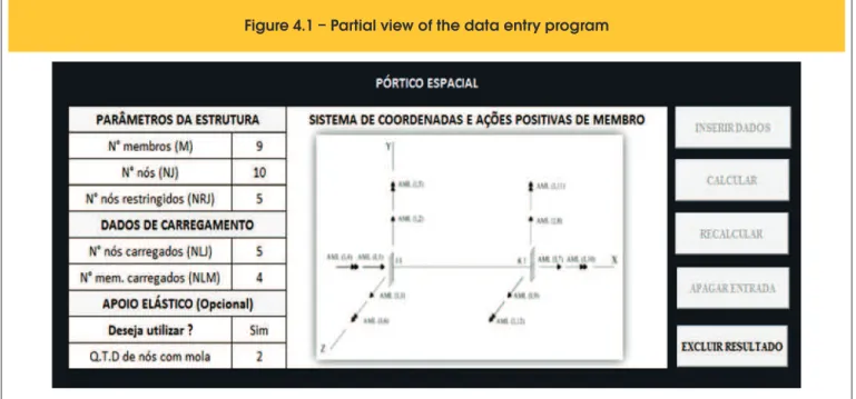
In this context, a program was developed in Visual Basic (VB), using Microsoft Excel ® platform, which considers the deformabi -lity of the adjacent soil to shallow foundations. The method is ba-sed on the assumption of Winkler, using discrete adjacent springs along the base of the foundations. This rheological model allows simulating the structure settlements and analyze the effects of the soil-structure interaction.
2. Soil-structure interaction
In Brazil the irst contextualization on this subject were made by Chamecki [5], which the main idea of the work was to establish a relationship between the stiffness of the structure and the foun-dation settlements. In the author words “Solidarity among the elements of the structure, gives the same considerable stiffness, which makes the differential settlement becomes less accented than the calculated [...]” (CHAMECKI, 1954, pg. 37). Based on this conception we realize that the eficiency of the project depends on the analysis of the interaction between the soil and the structure. The structural project idealized on a rigid base, without any displa -cement possibility, allows subdividing the building in three parts: su -perstructure, infrastructure and ground foundation. We note, throu-gh studies by Silva [6], this division is still making part of the structure analysis, in which the foundations are considered as elements ini -nitely rigid. This hypothesis is interpreted as independence between the parts, making the structural analysis not effective, because it limits the study of each subsystem in an isolation way [2].
calculator is worried only with the part above the ground, and the foundation engineer only with foundations elements and the adja-cent soils to themselves. However, the behavior of the building is related to the interaction between the interfaces of the model com-ponents (superstructure, infrastructure, soil mass), and this interfe-rence is deined as the mechanical phenomenon of soil-structure iteration (SSI).
Several authors have demonstrated the importance on structural analysis incorporated to the study of settlements, according to Velloso, Santa Maria and Lopes [8], this study “[...] aims to provide the real displacements of the foundation - and also of the structure if it is included in the analysis - and its internal efforts”. Therefore, it is essential the correct evaluation of the model support to become the construction project more realistic, taking into consideration the factors of interference between soil and structure.
3. Analysis of the soil deformability
To understand the effects of soil-structure interaction is necessary the comprehension of how the soil behaves when it is subjected the loads of ediication, as well as, their physical behavior during the loading process. During this process, in the understanding of Cintra, Aoki and Albiero [9], inevitably vertical displacements oc -cur, downwards, usually in order of centimeters, and in exceptional cases may reach hundreds of centimeters. This deformation in re-lation to rigid is called settlement.
According to Simons and Menzies [10] the foundation settlements may be considered as: immediate settlement (wi); primary conso-lidation settlement (wc) and secondary consolidation settlement (ws), w = wi + w c + w s. The immediate settlement is the predomi-nant portion of consolidation in sandy soils and is time indepen-dent. It results in the deformation almost instantaneous when the load is applied to the soil, without the occurrence of the reduction of the void ratio in soil mass. While soil is not an elastic material, because the settlements are not recovered by unload, the imme -diate settlement is calculated using the theory of elasticity due to the initial volume deformation be constant in the soil mass [6]. In low permeability soils, as in the case of saturated clays, great part of the foundation settlement is due to the consolidation of the subjacent layer. In the case of settlement by consolidation, both the primary and the secondary are time-dependent and result due to the reduction of the void ratio. The primary settlement occurs because of the dissipation of excess of neutral pressure present in the solid after loading, while the secondary settlement modiies the structure of the soil without having an increase in load, in other words, without increasing the effective stress. But despite the no -menclature used to differentiate them, it does not mean that they happen at different times [10].
3.1 Winkler model
This soil behavior model admits that the contact pressures are pro -portional to the displacement (w) of any point on the surface of the ground when loaded. For the case of vertical strain, the stress is given by Equation (1):
(1)
σ
=k
s
v
.w
i
Where:
σ is the average contact stress at the base of the foundation. wi is the vertical displacement (settlement).
kvs is the module vertical reaction. This value depending to the type of soil that form the bulk of the foundation.
These springs are represented by the coeficient of elastic support Ks (kN/m), which is directly proportional to the vertical reaction module Ki (kN/m³) and the loading area Af (m²), according to equation (2).
(2)
K
i
=
K
A
s
f
According to Moraes [11] it is possible to admit that the foundation base keeps rigid after the elastic deformation of the soil, which allows considering a linear variation of stress. Under these condi -tions, it is possible to calculate the displacements from the elastic support coeficients Ks (kN / m), according to the equation (3).
(3)
w=
K
N
V
=
F
K
s
v
.A
f
Where:
N is an action in the foundation base. F is é a normal force to the analyzed section. The reaction module Kv
s is not a constant of the soil and depends on various factors, such as: shape and size of the foundation, type of construction and load changes (MORAES, 1976). In general, the coeficient Kv
s can be determined in three ways: plate tests, tables of typical values and through correlations with elastic modulus. In the absence of appropriate tests Béton-Kalender (1962, apud MORAES [11]) recommends the use of the values in Table 3.1, for the vertical reaction module and values of the table 3.2, for the elasticity module (for soils subjected to a lower stress 1 MPa). These properties were obtained through the metal plate tests with a diameter of 45 cm.
The values proposed in the bibliography must be corrected, becau -se according to Velloso and Lopes [3], vertical reaction modules does not derive only from soil properties but also from a loading system, so they must be corrected for this situation, considering the size and shape of the analyzed element. The authors propose a correlation using equation (4), assuming the soil as an elastic homogeneous and semi-ininite material to approach the value to the real situation.
(4)
K
B
v
= K
b
v
.
b
B
I
s b
I
s B
Where: Kv
B is the vertical reaction module of the foundation; Kv
b is the vertical reaction module of the plate.
b is a smaller dimension of the plate; B is a smaller dimension of the foundation; Is
B is the shape material of the foundation;
Is
b is the shape factor of the plate.
v
Table 3.1 – Values of Ks
Type of soil
K (kN.m )
V -3 SLight peat - Marshy ground
Heavy Peat - Marshy ground
Fine sand beach
Landfill silt, sand and gravel
Soaked clay
Wet clay
Dry clay
Dry clay hardened
Compacted silt with sand and stone
Compacted sand and silt with many stones
Gravel with fine sand
Medium gravel with fine sand
Coarse gravel with coarse sand
Coarse gravel with little sand
Coarse gravel with little compacted sand
5,000 to 10,000
10,000 to 15,000
10,000 to 15,000
10,000 to 20,000
20,000 to 30,000
40,000 to50,000
60,000 to 80,000
The shape factors, are recommended by Perloff (1975, apud VELLOSO; LOPES [3]), as shown in Table 3.3 [3]. In case of pro -blems with thickness of inite compressible layer we use a similar table which can be obtained, in Velloso and Lopes [3].
The settlement (w) can also be obtained by a direct calculus, ba-sed on the theory of elasticity. According to Velloso and Lopes [3], this method is widely used in the analysis of SSI, and it is always associated with simpliied models of the soil behavior. The authors present for the settlement prediction, in footings under centered load, the equation (5).
(5)
w=q .B .
1-v²
E .I
s
.I
d
.I
h
Where:
w is the direct settlement; q is the medium applied pressure;
B is the smallest dimension of the foundation; υ is Poisson coeficient;
E is the elasticity module; Is is is the shape factor; Id is the embedded factor;
Ih is the thickness factor of the compressible layer.
The coefficient Is is a function of the footing shape and its stiffness. In the flexible case depends on the position of the point on the footing (center, edge, etc.) to which is desired the estimate of the immediate settlement. Thus, equation (5) can be used for rigid and flexible footing, with appropriate values of Is, presented in Table 3.3. The dimension characteristic of the footing, B, is taken by convention, as the diameter of the circular footing or as the length of the shorter side of a rectan-gular footing.
The shape factors (Is) are usually tabulated for certain values Id
and Ih. The Table 3.3 shows these values for the case of loading on the surface of a medium ininite thickness, where Id and Ih are equal
1.0. From the settlement it becomes possible the determination of the spring coeficient (Kv), applying the deformation obtained in the equation (3).
4. Methodological procedures
4.1 Program development
The initial step was the formalization of the computational pro -gram, based on the low charts presented by the authors Gere and Weaver Jr. [1], for space frame, using the stiffness method for the loads and displacements determination in frame structures. It was used the programming language of Visual Basic (VB) Microsoft
Table 3.2 – Values of E (endometrial elasticity module ) and E (elasticity module)
oValues of E and E
oE (MPa)
oE (MPa)
Peat
Soaked clay
Plastic clay
Hardened clay – plastic
Loose sand
Compact sand
0.1 to 0.5
1.5 to 4.0
4.0 to 8.0
8.0 to15.0
10.0 to 20.0
50.0 to 80.0
0.07 to 0.35
0.99 to 2.2
2.6 to 5.3
5.3 to 9.9
6.6 to13.2
33.0 to 53.0
Table 3.3 – Shape factors Is, for loadings on the surface in an infinite thickness way [12]
Shape
Rigid
Center
Edge
Average
Flexible
Circle
Square
Rectangle
L/B = 1,5
2
3
5
10
100
1000
10000
1.00
1.12
–
1.36
1.52
1.78
2.10
2.53
4.00
5.47
6.90
0.64
0.56
–
0.67
0.76
0.88
1.05
1.26
2,00
2.75
3.50
0.85
0.95
–
1.15
1.30
1.52
1.83
2.25
3.70
5.15
6.60
Excel ® platform. The main view of the developed software can be seen in Figure 4.1.
However, as the key requirement to validate the computational model is that it produces satisfactory results when compared to the results from the literature corresponding to the computational lowchart. Therefore, through an example of space frame, example I (5.1.1) available in the book Frame Structural Analysis by the authors Gere and Weaver, Jr. [1], a numerical test was performed.
4.2 Methodology for the lexible support inclusion
This procedure is done by replacing the rigid support by a lexible one, through replacing the degrees of freedom by a deined stiff -ness spring. This spring, partially constraints the displacement of a particular joint, thus characterizing a condition of elastic support.
4.3 Methodology for the consideration of the
soil-structure interaction
The technique consists in calculating the support reactions of the structure, with rigid support, and from these values estimate the di -mensions of the foundation to later apply the equation (5), to get im-mediate settlement. The elastic coeficient, for the base of each colu -mn, can then be obtained from equation (3). In a new analysis, rigid supports are replaced by the springs coeficients, at this point new reactions, new settlements and new springs coeficients are obtained. As the spring coeficients derive speciically from the type of soil and foundation dimensions, at each iteration, the foundation elements should be resized. The process is iterative and reaches the end when the settlements or support reactions converge to the same value. This procedure is based on the methodology presented by Chamecki [5].
4.3.1 Spatial model
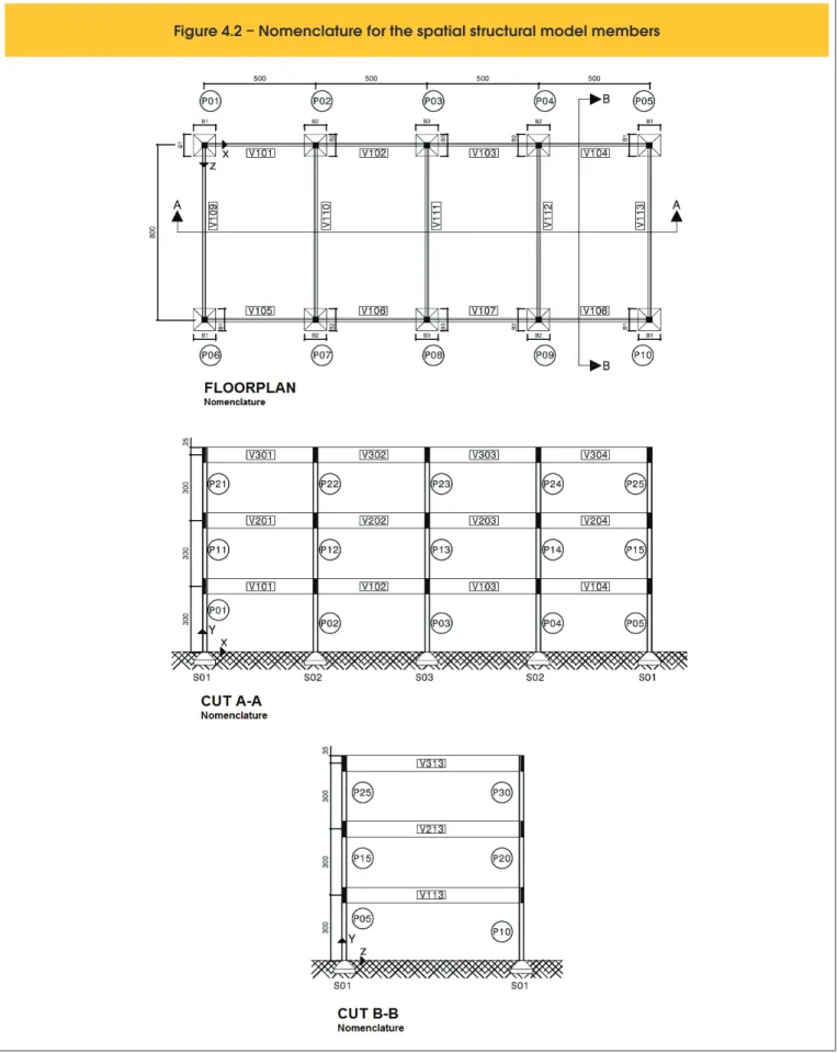
The spatial model, illustrated by the Figure 4.2, consists of
sixty--nine members and forty joints, initially the joints 1-10 will be cons-traints, then these vertical constraints will be replaced by relative stiffness coeficients, calculated as the equation (3) according to the elastic settlement of the points that rest on solid ground. Taking into consideration the loads, the spatial model uses only uniform loads Q, acting in the negative Y direction, applied to all horizontal structural members and all members are subject to ac -tions due to their own weight (γc = 25 kN/m³). The structural ele-ments are reinforced concrete with compressive strength (fck) de 25 MPa.
At the beginning, the model was submitted to the SSI analysis in si-tuations of homogeneous soil, in the speciic case, sand and clay. Then (in a characterized combination as a landill performed in a sideband in the transverse direction (Z) of the structure), the P01 columns (member 01) and P06 (member 06) were submitted to spring coeficients of lower stiffness than for the other columns. All the beams have dimensions of 15x70 cm, base and height res -pectively, while the columns have a section of 20x20 cm. The other physical parameters for the resolution since structural model are listed in Table 4.1. The numeration, location and nomenclature of the members and foundations can be seen in the Figure 4.2. Two types of mass soils are used in the analysis, a soil with less strength and other more strength capacity. The soil with less
stiff-Figure 4.1 – Partial view of the data entry program
Table 4.1 – General physical parameters
for the spatial structural model
Q (kN/m)
E (kN/m )
2G (kN/m )
230.0
L (m)
x5.0
28,000,000.00
L (m)
y3.0
11,666,666.70
L (m)
zness is clay with elasticity module (Es) of 35 MPa and Poisson’s coeficient equal to 0.3, with a resultant basic stress of 0.2 MPa. The most resistant soil is sand with elasticity module (Es) of 70 MPa and Poisson’s coeficient of 0.4, with a basic stress of 0.4 MPa. For purposes of calculus the footing will be considered on the ground surface and hinged, limiting the analysis only to the vertical displacements of each support.
5. Presentation and discussion
of the results
5.1 Program validation
5.1.1 Example I
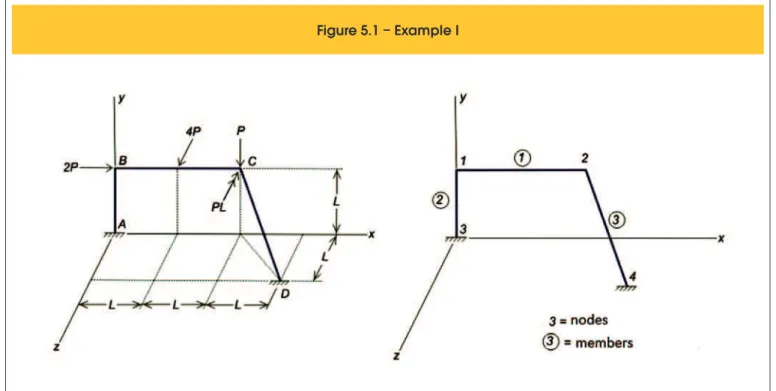
The irst example, shown in Figure 5.1 [1], consists of three mem -bers and four joints, where two are completely constrained (A and D), resulting in twelve support constraints, the rest are free getting twelve degrees of freedom to the structure (six in each of the joints B and C). The joint loads consist of: 2P in the positive direction of the X axis, in point B; P in the negative direction of the Y axis, at
point C, and a torque PL in the negative direction of the Z axis at the point C. Further, on BC member, there is a load of 4P in the positive Z direction, applied at the gap of each member.
The physical parameters for this structural model resolution are shown in Table 5.1 (Gere and Weaver Jr. [1]).
The results generated by the software, for the displacements and reactions of the example I, are shown in table 5.2.
The results for the displacements and reactions of the example I, according to Gere and Weaver Jr. (1987, p. 366), can be observed in Table 5.3 [1].
It is possible to observe the compatibility between the results pre -sented by Gere and Weaver Jr. (1987, p. 366) and the results ob -tained with the developed software. It is important to highlight that other examples were analyzed and all the results are compatible with the literature, not being added to the present work, for not writing too much text.
5.2 Results for the spatial model
From the support reactions obtained from the spatial model, for each combination under rigid and lexible base, considering the described methodology for the consideration of the soil-structure interaction (item 4.3), tables for each iteration and to each column were developed. The convergence process, for the lateral landill combination (P01/P06), can be seen in Table 5.4.
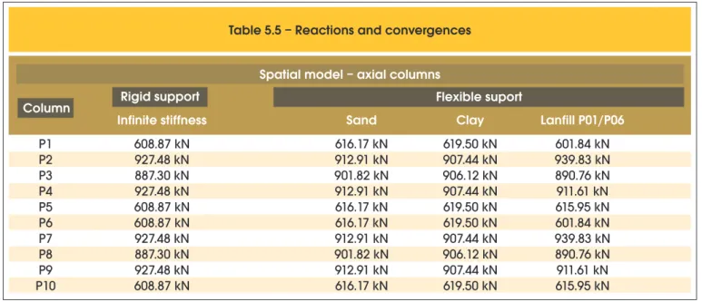
Applying to the methodology again it was created the table 5.5, which presents a summary table of the inal reactions for all the cases proposed on item 4.3.1.
The structure behavior can be analyzed from the variation percen -tage of the three combinations, for the column reactions, in relation to the efforts obtained in the situation of rigid support. Figure 5.2 has as objective demonstrate the effort migration according to the elastic base (P01/P06 combination simulates a lateral landill ac -cording to the item 4.3.1.)
ample I
Table 5.1 – Example data I
E (MPa)
G (MPa)
P (kN)
L (m)
A (m
x²
)
4
I (m )
x4
I (m )
y4
I (m )
z206,842.71
82,737.08
4.45
3.5
0.0071
-5
3.45.10
-5
2.33.10
-5
Table 5.2 – Displacements and reactions of the example I
Joint
Trans. X
Load X
Trans. Y
Load Y
Trans. Z
Load Z
Bending X
Rot. X
Bending Y
Rot. Y
Bending Z
Rot. Z
Joint, displacements (m e rad/m) and Reactions (kN e kN.m)
1
2
3
4
-0.00388112
0
-0.00391674
0
0
-0.396
0
-8.762
0.00000618
0
0.01158629
0
0
-2.980
0
7.43
0.01590856
0
0.01559181
0
0
-9.038
0
-8.762
0.0001914
0
0.0000910
0
0
-25.694
0
-2.903
-0.0001387
0
0.0001459
0
0
5.123
0
-5.032
0.0000679
0
-0.0000686
0
0
-3.628
0
3.50
Table 5.3 – Displacements and reactions of the example I, according to the bibliography
Joint
Trans. X
Load X
Trans. Y
Load Y
Trans. Z
Load Z
Bending X
Rot. X
Bending Y
Rot. Y
Bending Z
Rot. Z
Joint, displacements (m e rad/m) and Reactions (kN e kN.m)
1
2
3
4
-0.0038811
0
-0.0039167
0
0
-0.4
0
-8.76
0.0000062
0
0.0115863
0
0
-2.98
0
7.43
0.0159085
0
0.0155918
0
0
-9.04
0
-8.76
0.000191
0
0.000091
0
0
-25.69
0
-2.90
-0.000139
0
0.000146
0
0
5.12
0
-5.03
0.000068
0
-0.000069
0
0
-3.63
0
3.50
Table 5.4 – Stiffness, coefficients, reactions and foundation elements
Column
Rigid support
Combination – lateral landfill - P01/P06
Flexible support
Iteration 1
K
v -1(kN.m )
K
v -1(kN.m )
K
v -1(kN.m )
Rv (kN)
Footing (m)
Rv (tf)
Footing (m)
Rv (kN)
Footing (m)
The variations of the results show a trend of uniformity of the loa -ds. It is possible to see that the soil with lower reaction coeficient causes greater effort redistribution. However, it should be noticed that the magnitude of the effort redistribution was not so signiicant, due to the large foundation dimensions and, consequently, more rigid. The variations reached a maximum of 2.08% for increases and a minimum of -2.21% for alleviations, both while the model was seated on the clay.
In the combination between two types of soil, where P01 and P06 columns are submitted to a lower stiffness coeficient compared to the other, it is seen the inluence of the structure rotation in its behavior, causing load alleviations in order of 1.17% in P01 and P06 columns and overloading the neighboring columns, P02 and P08, in the order of 1.31%.
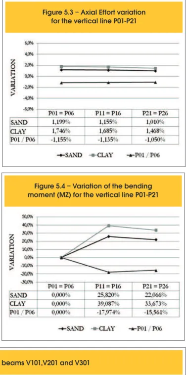
The behavior of the efforts, according to the loor increase, can be observed through P01-P21 vertical lines, symmetrical to the verti -cal lines P06-P26. Normal and bending efforts acting on the base of the columns, analyzed in module due to the symmetry of the reforced arrangement, are listed respectively in tables 5.6. On the other hand the discrete variation in normal efforts of the columns, the moments had a signiicant increase, in relation to rigid situation, reaching up to 39.087% on the clay base. Atte -nuating moments in the transversal direction of the spatial mo -del showed no change compared to the efforts obtained with the model of ixed supports, justiied by the absence of rotation in transversal members.
The vertical lines behavior P01-P21, through each loor, can be seen in the graphs presented in the igures 5.3 and 5.4.
Table 5.5 – Reactions and convergences
Column
Rigid support
Spatial model – axial columns
Flexible suport
Infinite stiffness
608.87 kN
927.48 kN
887.30 kN
927.48 kN
608.87 kN
608.87 kN
927.48 kN
887.30 kN
927.48 kN
608.87 kN
Sand
Clay
Lanfill P01/P06
616.17 kN
912.91 kN
901.82 kN
912.91 kN
616.17 kN
616.17 kN
912.91 kN
901.82 kN
912.91 kN
616.17 kN
619.50 kN
907.44 kN
906.12 kN
907.44 kN
619.50 kN
619.50 kN
907.44 kN
906.12 kN
907.44 kN
619.50 kN
601.84 kN
939.83 kN
890.76 kN
911.61 kN
615.95 kN
601.84 kN
939.83 kN
890.76 kN
911.61 kN
615.95 kN
P1
P2
P3
P4
P5
P6
P7
P8
P9
P10
Table 5.6 – Acting efforts in the vertical lines members P01-P21
Column
Column
Rigid support
Spatial model – vertical lines efforts P01-P21
Flexible support
Flexible support
Infinite stiffness
Clay
N
N
N
N
MY
MY
MY
MY
MZ
MZ
MZ
MZ
608.87 kN
407.03 kN
202.93 kN
619.50 kN
413.89 kN
205.91 kN
616.17 kN
411.73 kN
204.98 kN
601.84 kN
402.41 kN
200.80 kN
0.00 kN.m
30.56 kN.m
30.54 kN.m
0.00 kN.m
30.56 kN.m
30.54 kN.m
0.00 kN.m
30.56 kN.m
30.54 kN.m
0.00 kN.m
30.56 kN.m
30.54 kN.m
0.00 kN.m
7.01 kN.m
7.84 kN.m
0.00 kN.m
9.75 kN.m
10.48 kN.m
0.00 kN.m
8.82 kN.m
9.57 kN.m
0.00 kN.m
5.75 kN.m
6.62 kN.m
Sand
P01 / P06
P01 = P06
P11 = P16
P21 = P26
According to the variations, gotten through each loor, it is possible to observe that independently of the combination or the vertical line analyzed, the variations are bigger in the members closer to the foundations. It happens because of the increase on the stiffness structure, proportionally to the loor increase, which causes lower rotations.
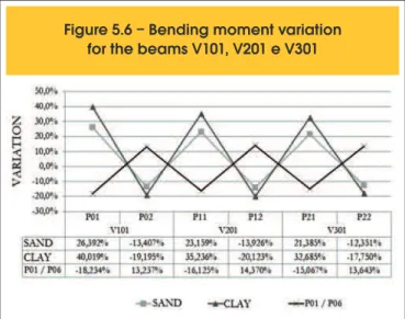
To analyze the beams behavior was selected longitudinal referen -ce beams (X-axis). The beams are V101-V301, symmetric the be-ams V305-V105, in the longitudinal direction. The shearing efforts are related in Table 5.7 and its variations are represented by the graph in igure 5.5.
The bending moments can be seen in table 5.8 and its variations are presented in Figure 5.6.
Analyzing the igures 5.5 and 5.6 it is possible to see that the shearing efforts did not have signiicant variation percentage. Ho -wever, the high bending moment variation is due to the direct in -luence of the rotation of the ends, which is higher in the case of lexible support. It is also notable the reduction variation with the
Figure 5.2 – Graphical analysis of the percentage change
of the vertical reactions of the spatial structural model
Figure 5.3 – Axial Effort variation
for the vertical line P01-P21
Figure 5.
4 – Variation of the bending
moment (MZ) for the vertical line P01-P21
Table 5.7 – Shear effort for the beams V101,V201 and V301
Beam
Rigid support
Spatial model – shearing
Flexible support
Infinite stiffness
68.3 kN
94.8 kN
70.6 kN
92.5 kN
69.4 kN
93.7 kN
Sand
Clay
Lanfill P01/P06
70.9 kN
92.2 kN
73.3 kN
89.9 kN
71.5 kN
91.6 kN
72.1 kN
91.0 kN
74.5 kN
88.7 kN
72.4 kN
90.7 kN
65.9 kN
97.2 kN
68.1 kN
95.0 kN
67.3 kN
95.8 kN
P01
P02
P11
P12
P21
P22
V101
V201
Figure 5.5 – Shearing effort variation
for the beams V101, V201 e V301
Figure 5.6 – Bending moment variation
for the beams V101, V201 e V301
Table 5.8 – Bending moments for the beams V101, V201 e V301
Beam
Rigid support
Spatial model – bending moments
Flexible support
Infinite stiffness
10.4 kN.m
-76.5 kN.m
15.1 kN.m
-69.9 kN.m
8.20kN.m
-68.9 kN.m
Sand
Clay
Landfill P01/P06
13.2 kN.m
-66.3 kN.m
18.6 kN.m
-60.1 kN.m
10.0 kN.m
-60.4 kN.m
14.6 kN.m
-61.8 kN.m
20.4 kN.m
-55.8 kN.m
10.9 kN.m
-56.7 kN.m
8.50kN.m
-86.7 kN.m
12.6 kN.m
-79.9 kN.m
7.00kN.m
-78.3 kN.m
P01
P02
P11
P12
P21
P22
V101
V201
V301
increasing loors, that is justiied by the convergence of displace -ments between the rigid and lexible analysis, making variations become negligible according to the analysis of the structure moves away from the interface with the foundations.
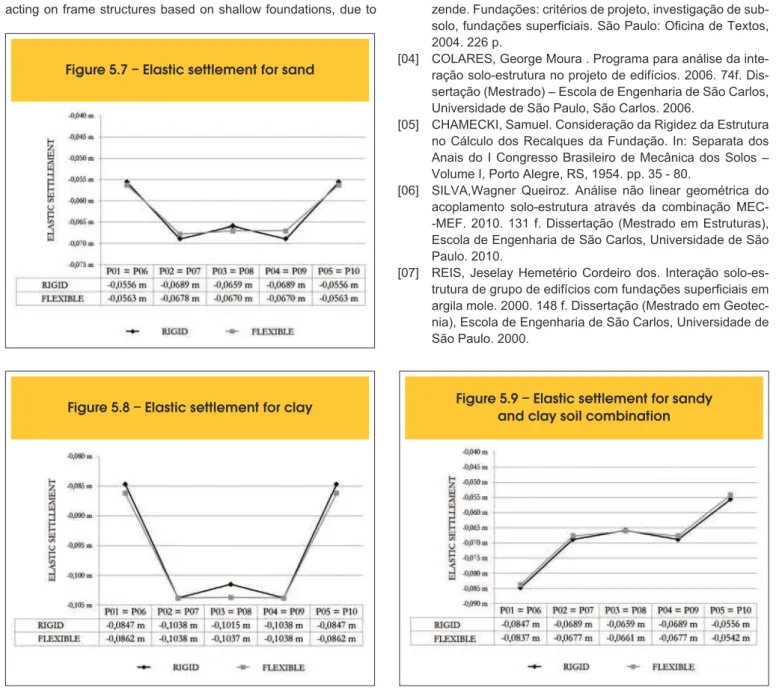
Performing the immediate settlements analysis of the foundations model it also realizes the uniformity of settlements to the lexible support situations. The settlements values are related between le -xible and rigid support, for sand, clay and soil combination of both, according to igures 5.7, 5.8 and 5.9. The base for foundation is regarded as 0.00 m quota.
The uniformity of settlements caused by the compatibility between soil and structure is observed that the differential settlements be -come smaller. The differential settlements obtained for the spatial model do not exceed distortions larger than 0.0352% (maximum differential settlement between P01 and P02, respective to the le -xible support situation on clay).
6. Conclusions
Winkler solution, used for getting stiffness coeficients for foun -dations, admits the soil as an elastic, homogeneous, semi-ininite material, which responds elastically to the loading. However, it is
known that the soil does not recover the original volume in the unloading of itself, due to permanent deformation of the structure. However, limiting the stress at the base of the foundation to admis -sible stress it is pos-sible to consider an elastic soil response. At this contest, this rheological model was presented as a relatively simple and practical solution, due to the convergence of the results in a few iterations.
The comparative analysis of the results showed that the efforts redistribution is proportional to the rotations suffered by elements of the model.
In general, soils with lower reaction coeficient cause larger effort redistributions, forcing its compatibility according to the stiffness of the springs placed at the base of each column. However, the elastic constants used to simulate the deformation of the soil, ne-glect the interaction between adjacent springs, so the errors tend to grow on soft soils.
-settlement at the supports, rotating the beams and causing the migration of the load to the neighboring columns, with smaller settlements, which would not happen if the supports had iden-tical settlements.
It is clear that the redistribution effects are more accented at the ends of the beams than in the columns. The stiffness inluence of the horizontal elements is also notable in the load redistribution, since the efforts transfer occurs through the same, so as high the stiffness of the beams is as near the structure behavior will be of a rigid block.
The variations in the efforts are higher for the members closer to the foundations, independently of the combination. It happens be-cause of the increase of the stiffness structure with the increase on the loors, therefore a factor to be considered in the beams transition project.
In this context, it was proved that there is variation in the efforts acting on frame structures based on shallow foundations, due to
portance of considering this phenomenon in situations with high concentration of normal effort, which would cause high differentials settlements, whose effects would be neglected in a conventional analysis. Therefore, even with the use of a simpliied model, it is concluded that disregard the inluence of the support settlements can conduct to non-realistic efforts able to harm the safety and the durability of the buildings.
7. References
[01] GERE, James M.; WEAVER JR., William. Análise de Estru -turas Reticuladas. Rio de Janeiro: Guanabara, 1987. 443 p. [02] GUSMÃO, Alexandre Duarte. Aspectos relevantes da inte -ração solo-estrutura em ediicações. Rev. Solos e Rochas, São Paulo, v. 17, n. 1, p. 47-55, 1994.
[03] VELLOSO, Dirceu de Alencar; LOPES, Francisco de Re -zende. Fundações: critérios de projeto, investigação de sub -solo, fundações supericiais. São Paulo: Oicina de Textos, 2004. 226 p.
[04] COLARES, George Moura . Programa para análise da inte -ração solo-estrutura no projeto de edifícios. 2006. 74f. Dis -sertação (Mestrado) – Escola de Engenharia de São Carlos, Universidade de São Paulo, São Carlos. 2006.
[05] CHAMECKI, Samuel. Consideração da Rigidez da Estrutura no Cálculo dos Recalques da Fundação. In: Separata dos Anais do I Congresso Brasileiro de Mecânica dos Solos – Volume I, Porto Alegre, RS, 1954. pp. 35 - 80.
[06] SILVA,Wagner Queiroz. Análise não linear geométrica do acoplamento solo-estrutura através da combinação MEC --MEF. 2010. 131 f. Dissertação (Mestrado em Estruturas), Escola de Engenharia de São Carlos, Universidade de São Paulo. 2010.
[07] REIS, Jeselay Hemetério Cordeiro dos. Interação solo-es -trutura de grupo de edifícios com fundações supericiais em argila mole. 2000. 148 f. Dissertação (Mestrado em Geotec -nia), Escola de Engenharia de São Carlos, Universidade de São Paulo. 2000.
Figure 5.7 – Elastic settlement for sand
[08] VELLOSO, Dirceu de Alencar; SANTA MARIA, Paulo Edu -ardo Lima de; LOPES, Francisco de Rezende. Princípios e modelos básicos de análise. In: HACHICH, Waldemar. Fun-dações: teoria e prática. 2. ed. São Paulo: PINI, 1998. p. 163-196.
[09] CINTRA, José Carlos A.; AOKI, Nelson; ALBIERO, José Henrique. Tensão admissível em fundações diretas. São Carlos: Rima, 2003. 134 p.
[10] SIMONS, Noel E.; MENZIES, Bruce K.. Introdução à engenha -ria de fundações. Rio de Janeiro: Interciência, 1981. 199 p. [11] MORAES, Marcello da Cunha. Estruturas de fundações. 2.
ed. São Paulo: McGraw Hill, 1976. 205 p.
![Table 3.3 – Shape factors Is, for loadings on the surface in an infinite thickness way [12]](https://thumb-eu.123doks.com/thumbv2/123dok_br/18860622.417865/4.892.62.833.856.1133/table-shape-factors-loadings-surface-infinite-thickness-way.webp)