WORKING PAPER SERIES
CEEAplA WP No. 14/2008
High Speed Rail Transport Valuation
Pedro Pimentel
José Azevedo-Pereira
Gualter Couto
High Speed Rail Transport Valuation
Pedro Pimentel
Universidade dos Açores (DEG)
e CEEAplA
José Azevedo-Pereira
Departamento de Gestão e CIEF,
Instituto Superior de Economia e Gestão
Gualter Couto
Universidade dos Açores (DEG)
e CEEAplA
CEEAplA Working Paper n.º 14/2008
Novembro de 2008
RESUMO/ABSTRACT
High Speed Rail Transport Valuation
The present paper investigates the optimal timing of investment for a high
speed rail (HSR) project, in an uncertain environment, using a real options
analysis (ROA) framework. It develops a continuous time framework with
stochastic demand that allows for the determination of the optimal timing of
investment and the value of the option to defer in the overall valuation of the
project. The modelling approach used is based on the differential utility provided
to railway users by the HSR service.
Keywords: Real Options, Uncertainty, Timing, Waiting, Investment, High
Speed Rail.
JEL classification: D81, D83, D92.
Pedro Pimentel
Departamento de Economia e Gestão
Universidade dos Açores
Rua da Mãe de Deus, 58
9501-801 Ponta Delgada
José Azevedo-Pereira
Departamento de Gestão
Instituto Superior de Economia e Gestão
Universidade Técnica de Lisboa
R. Miguel Lupi,
1249-078 Lisboa
Gualter Couto
Departamento de Economia e Gestão
Universidade dos Açores
High Speed Rail Transport Valuation
Pedro Miguel PimentelË University of the Azores
Business and Economics Department, CEEAplA,
R. Mãe de Deus, 9500 Ponta Delgada, Portugal, [email protected] José Azevedo-Pereira
ISEG
Universidade Técnica de Lisboa Department of Management
R. Miguel Lupi, 1249-078 Lisboa, Portugal, [email protected] Gualter Couto
University of the Azores,
Business and Economics Department, CEEAplA
R. Mãe de Deus, 9500 Ponta Delgada, Portugal, [email protected]
This draft: October 2007
ABSTRACT
The present paper investigates the optimal timing of investment for a high speed rail (HSR) project, in an uncertain environment, using a real options analysis (ROA) framework. It develops a continuous time framework with stochastic demand that allows for the determination of the optimal timing of investment and the value of the option to defer in the overall valuation of the project. The modelling approach used is based on the differential utility provided to railway users by the HSR service.
Keywords: Real Options, Uncertainty, Timing, Waiting, Investment, High Speed Rail. JEL classification: D81, D83, D92.
Ë
1. Introduction
In uncertainty environments flexibility is crucial to perform efficiently, for instance, in terms of technological changes, competition’s shifts, or even in order to limit potential losses related to unexpected adverse scenarios in the market (Trigeorgis, 1996).
In spite of having emerged in the academy, (Brennan and Schwartz, 1985; McDonald and Siegel, 1986; Dixit, 1989; Pindyck, 1991; and Dixit and Pindyck, 1994, amongst others), the real options analysis has already made an impact in the business world, since an increasing number of companies and managers are adopting a real options perspective. Especially in capital budgeting decisions and in the assessment of the corresponding strategic positioning and competitiveness (Paddock, Siegel and Smit, 1988; Nichols, 1994; Kallberg and Laurin, 1997; Moel and Tufano, 2002; Smit, 2003; etc.).
The modelling framework proposed in this paper is inspired by a set of projects for the development of high speed rail (HSR) lines in Europe. The structuring nature of the projects for the countries involved; the need to renew the railway sector; the huge amounts of money needed; the uncertainty about the timings to invest and the economic challenge inherent in developing a conceptual setting for a decision that needs to be taken in the interest of the entire set of European taxpayers, all play a part in providing relevance to the study of the embedded option to defer and the optimal timing to invest.
In section 2 we present the literature regarding real options in major projects in the transportation sector. The valuation framework is developed in section 3. After providing numerical results in section 4, section 5 concludes the paper.
2. Real Options in Major Projects in the Transportation Sector
Although usually linked to political discussion and controversy, transport infrastructures tend to be understood as critical for the sustainable growth and development of any economy. According to Wilson (1986), since 1870 economists have been drawing their attention towards the transport industry in general, and to the railway sector in particular. The same author suggests that wrong transportation policies and the corresponding investment mistakes in transport infrastructures may compromise
seriously economic growth. To prevent this type of outcome, it is important to develop and apply suitable decision criteria based upon sound cost/benefit analysis.
Infrastructure investments that are usually understood to provide benefit and leverage to the economic growth of whole regions include investments in seaports, airports and railways links, energy networks, road systems, amongst others.
The size, budget and impact in the global economic activity lead big transportation investments to assume the role of strategic options. Almost all these investments include a portfolio of options intended to, at some extent, protect the enormous funds needed to implement the project from failure.
Rose (1998) has valued the concession of a toll road, considering the existence of two options interacting with each other. The author assumed that the traffic volume followed a geometric Brownian motion and used Monte Carlo simulation to compute i) the value of the embedded call option that allowed for the early acquisition of the project by the franchiser and ii) the option to defer regarding the payment of the corresponding fees’ by the franchisee. Similarly, Brandão (2002) applied the Copeland and Antikarov’s (2003) framework to value several options embedded in a project that included the building and operation of highways in Brazil.
More recently, two other empirical ROA works focused on the valuation of structural investments in the transportation sector, were published: Smit (2003) and Bowe and Lee (2004). The first, analyses the expansion of an airport, while the second is apparently pioneer in the analysis of a railway transportation project.
Investments in infrastructure or platform assets generate other investments opportunities that change the competitive standing of the companies involved. Smit (2003) combines ROA and game theory, in a discrete time framework, to capture the intrinsic value derived from the company’s positioning adjustment inside the industry, with an empirical application to the expansion of a European airport. His work has helped to fill in a gap in the real options literature, where researchers have tended to, either, ignore competition, underestimating the impact of a competitive entry, or assume that the competition is exogenous to the valuation process.
Similarly to Smit (2003), Bowe and Lee (2004) apply binomial analysis. However, they use a logarithmic transformation similar to Trigeorgis (1991), to evaluate the high speed train project in Taiwan, comparing the obtained results with a valuation based on traditional capital budgeting decision techniques. The work embraces the valuation of
three different options (expand, reduce and defer) and the according interactions, included in a project that does not pay dividends.
Compared to the literature reviewed, our paper introduces in transport valuation field the HSR investment analysis in continuous time, providing some closed form solutions. Although Pereira et al. (2006) present some research on these issues, their work focus in an airport construction project and includes other uncertainty factors.
3. Investment Valuation Using a Real Options Framework
In a HSR project, at any moment in time, the owner of the investment’s rights holds the possibility of acquiring the future cash flow generated by the venture, in exchange for the payment of the corresponding implementation costs. Thus, we are dealing with an option to invest.
Considering the investment in a HSR line as an optimal stopping problem allows us to determine the value of the embedded option to defer. Following, the work of McDonald and Siegel (1986) and Salahaldin and Granger (2005), it also permits to determine the optimal timing to invest.
In the present paper it will be assumed not only that the option to defer is perpetual in nature (T =∞), but also that, once implemented, the investment will produce perpetual benefits. Without major technological changes, the impact of these assumptions in the global valuation should not be unreasonable for two reasons. In the first place, because the present value of the more remote cash flows tends naturally to zero. In the second place, because maintenance and conservation - whose expenses are taken into consideration - tend to restore the operational aptitude of the assets in place and the corresponding flow of benefits.
3.1. Optimal Timing to Invest – Investment in one Period
In a context of the nature above mentioned, a decision to implement a project in a non-optimal moment, implies destruction of value. Therefore, finding the optimal timing offers the possibility to study the impact of the ability to delay in the global value of the project.
Thus, it is important to answer the question of when to invest, or at least find a critical value that might support in a rational way the decision of implementing the
investment. The irreversibility features of the investment, given that there is no other use for the project rather than the railways, emphasise the importance of estimating the optimal timing to invest.
The model proposed here draws on the work of Salahaldin and Granger (2005) on the valuation of sustainable systems of urban transport aimed at relieving air pollution. It is a model that comprises a unique change from an inactive to an active state, and considers a single stochastic variable.
Because investment in infrastructures, like HSR lines, will affect the economic and social conditions of future generations, it should be assessed considering a global point of view, in terms of economic welfare. In an uncertain environment, it will only make sense to invest in such a project, if the economic value of the utility provided by the resulting benefits is able to surpass the joint value of the option to defer (lost by investing) and of the utility provided by the conventional railway system to its users.
Investing, in a moment other than the corresponding optimal timing, implies a reduction in the global level of utility achieved by the users, compromising seriously the projects’ success. In such circumstances, any potential user may always maintain his current level of utility, choosing to travel in the conventional railway line, rather than in the new HSR service. If a suboptimal investment timing is chosen, the ability of the HSR service to attract clients will be strongly distressed.
At any moment users can choose to travel in the conventional railway, without any constraints. Consequently, to maintain the users’ utility, the fraction of the new investment supported by each one must be identical to the sum of the benefits earned resulting from the reduction of the travel time and the conventional service fare saved, net of variable and fixed operational costs upheld.
Given a fixed amount to invest, the higher the demand, the higher the expected net benefit per capita. Consequently, higher levels of demand tend to lead to the anticipation of the optimal invest timings. The main source of uncertainty derives obviously from the level of future demand for the HSR service.
We will consider that the demand for the new high speed service, x , follows a t
geometric Brownian motion process:
t t x t x t xdt xdw dx =µ +σ (1)
Similar assumptions may be found in Rose (1998), with the purpose of modelling highway traffic; in Salahaldin and Granger (2005), with the purpose of modelling the dynamics of a city’ population; and in Marathe and Ryan (2005) and Pereira et al. (2006) with the purpose of modelling airline demand.
In equation (1) µx and σx represent the growth rate and the standard deviation of
the demand for the HSR service. We assume that both parameters are constant in time. The Wiener process, w , has zero mean and standard deviation t σx dt.
Under these circumstances, it is reasonable to expect that, in the future, the natural demand for HSR will reach a level capable of providing a rational reason to invest in such a project.
In order to model such a situation we are going to assume that each user will face a cost for railway travel between two cities, ψ, whose global worth will be a function of the value of time for the user, η, and the travel fare, p . According to the literature, both these variables exhibit a relationship to the global demand for railway services (vide Owen and Phillips, 1987; Wardman, 1994; and Wardman 1997).
Considering the relationship between the value of travel time and the demand for faster railway services (Owen and Phillips, 1987; and Wardman, 1994), the following functional form will be used:
( )
β δβη xt = xt (2)
In this functional form, δβ represents the elasticity between the value of travel time
η and the HSR demand x . Consequently, β is the scale parameter between demand,
x , and the value of travel time, η.
Concerning the relationship between the fare value and the demand for railway services, this will be given by the functional form (Owen and Phillips, 1987):
( )
α δα tt x
x
p = (3)
The elasticity between the fare value, p , and the HSR demand, x , is represented by the parameter δα. The scale parameter α relates demand x and the fare value p .
The demand may be inferred from the preferences of a risk neutral representative user, with a utility function U
( )
c = . This utility is assumed to be a function of solely cthe mean consumption per user, in which c represents the mean consumption of all
users that constitute the overall demand. The budget constraint is given by:
( )
t tt c x
m = −ψ (4)
in which ψ represents the travel cost and m the individual disposable income by
unit of time.
Replacing the level of consumption in the utility function, will allow for the determination of the following utility function, V , representative of the value that each user attributes to a railway trip:
( )
xt U( )
ct mt( )
xtV = = −ψ (5)
The relationship between demand x and value of travel time, i) in the period of t
time that precedes investment, η0; ii) during the period of effective investment, η1; and
iii) after the investment’s implementation, η2, is represented, respectively, by β0, β1
and β2. Since the new rail service will save travel time and, in consequence, will
reduce the value of travel time from η0 to η2, it will be reasonable to expect that from
the pre-investment period to the operational phase β0 will change to β2 with β0 >β2.
The difference between β0 and β2 reflects the decrease in travel time.
Meanwhile, for the moment, we will assume that the investment will take place during a single period of time. Thus, the relationship between demand and travel costs, during the construction period β1 is assumed to be equal toβ2.
Analytically, the cost of travelling in a conventional railway, ψ0, and the cost of
travelling in HSR, ψ2, will be represented by the following equations,
( )
β δβ α δαψ0 xt = 0xt + 0xt (6)
( )
β δβψ2 xt = 2xt (7)
For modelling purposes, the conventional railway travel cost, ψ0, includes both the
value of the travel time lost and the fare paid. In contrast, the HSR travel cost function here considered, ψ2, is not affected by the value of the corresponding fare, p , because 2
the current valuation framework assumes implicitly that each user will bear his part of the investment expenditure plus the corresponding operating costs per user. In other
words, a socially acceptable HSR service fare is already implicitly considered in the valuation framework. Consequently, it does not make sense to duplicate it.
The existing conventional railway service that charges a fare p , enables us to 0
identify the relationship between HSR demand, x , and the price of a substitute service t
(Owen and Phillips, 1987; and Wardman, 1997) given by equation (3).
As long as the investment is not implemented, the utility function will be given by:
( )
β δβ α δα t t t t m x x x V0 = − 0 − 0 (8)After the investment is implemented, users will continue to face a (smaller) cost in terms of time spent. However, since the analysis performed here takes into consideration all costs and benefits induced by the project (including not only capital investment expenditure, but also all fixed and variable operating costs), the new utility function will be given by:
( )
t t t t t x x x m x V = −β δβ −ω− ϕ −ργ 2 2 (9)with γ representing the capital investment expenditure, ρ the discount rate, ω the variable operating costs and ϕ the fixed operating costs. Notice that
t x ϕ and t x ργ
represent the fixed operating costs and the investment expenditure per unit of time, for each user that integrates the global demand for the HSR service. We assume implicitly that the outcomes of the investment will last for an unlimited time horizon.
The purpose is to carry out the investment without changing the present utility function equilibrium. In order to achieve this outcome, it will be necessary to find the critical demand level for x , above which it will be optimal to invest. ∗
Noting that, in these terms, the whole framework might be understood as an intergeneration welfare problem, as previously stated, we may use the objective function of Ramsey-Koopmans adopted by Salahaldin and Granger (2005). Analytically, we have:
( )
( )
⎟⎠⎞ ⎜ ⎝ ⎛∫
− +∫
+∞ − ∗ τ ρ τ ρ dt e x V x dt e x V x E t t t t t t x x 2 0 0 sup (10) Where,time;
( )
xtV0 = Utility function per unit of time before investment implementation,
given by the equation (8);
( )
xtV2 = Utility function per unit of time after investment implementation,
given by the equation (9); and
t
x = Demand throughout time, given by the equation (1); and
Aggregating the utility of all users that constitute the potential demand before and after the investment, and replacing
0
V and V for the corresponding values in (8) and 2
(9), we get:
[
]
[
]
⎟⎠⎞ ⎜ ⎝ ⎛∫
− − − +∫
+∞ − − − − − ∗ τ θ ρ τ ρ θ θ ργ ϕ ω β α β β α β dt x x x m e dt x x x m e E t t t t t t t t t t x x 2 0 0 0 sup (11) with θβ = 1+δβ and θα =1+δα.Decomposing the first element of (11), we obtain
[
]
[
]
[
]
⎟⎟ ⎟ ⎠ ⎞ ⎜ ⎜ ⎜ ⎝ ⎛ − − − − + + − − − − −∫
∫
∫
∞ + − ∞ + − ∞ + − ∗ τ θ ρ τ θ θ ρ θ θ ρ ργ ϕ ω β α β α β β α β α β dt x x x m e dt x x x m e dt x x x m e E t t t t t t t t t t t t t t t x x 2 0 0 0 0 0 sup (12) Simplifying (12), the objective function comes as follow,[
]
[
(
)
]
⎟⎠⎞ ⎜ ⎝ ⎛∫
+∞ − − − +∫
+∞ − − + − − − ∗ τ θ θ ρ θ θ ρ β β α α β β β α α ω ϕ ργ dt x x x e dt x x x m e E t t t t t t t t t x x 0 2 0 0 0 0 sup (13) Since the first component does not depend on τ and x , the problem may be ∗rewritten, in the following terms:
(
)
[
]
⎟⎠⎞ ⎜ ⎝ ⎛∫
+∞ − − + − − − ∗ τ θ θ ρ β β β α α ω ϕ ργ dt x x x e E t t t t x x 0 2 0 sup (14)This objective function maximizes the net gain provided by an investment in a HSR link, in terms of travel costs for the corresponding users.
Let,
( )
∗ = ⎜⎝⎛∫
+∞ −[
(
−)
+ − − −]
⎞⎠⎟ τ θ θ ρ β β β α α ω ϕ ργ dt x x x e E x v t t t t x 0 2 0 (15)Applying the strong Markov property as in Oksendal (2003) in RHS, we will get:
(
)
[
]
(
)
[
]
⎟⎠⎞ ⎜ ⎝ ⎛ − + − − − = = ⎟ ⎠ ⎞ ⎜ ⎝ ⎛ − + − − −∫
∫
∞ + − ∞ + − ∗ 0 0 2 0 0 2 0 dt x x x e E dt x x x e E t t t t x t t t t x ργ ϕ ω α β β ργ ϕ ω α β β α β α β θ θ ρ τ θ θ ρ (16) In view of dominated convergence theorem, we have:(
)
[
]
(
)
( )
( )
( )
[
]
∫
∫
∞ + − ∞ + − − − − + − = = ⎟ ⎠ ⎞ ⎜ ⎝ ⎛ − + − − − ∗ ∗ ∗ ∗ 0 0 2 0 0 0 2 0 dt x E x E x E e dt x x x e E t x t x t x t t t t t x ργ ϕ ω α β β ργ ϕ ω α β β α β α β θ θ ρ θ θ ρ (17)We know that x follows a geometric Brownian motion described by (1). Thus, t
( ) ( )
( ) ⎟ ⎠ ⎞ ⎜ ⎝ ⎛ + − ∗ = ∗ t t t x x x e x x E 2 1 2 1θθ σ µ θ θ θ (18)The existence of a future optimal timing to invest requires the need to respect the following condition
(
1)
02
1 − 2>
−
−θµx θ θ σx
ρ . This condition imposes the demand
growth rate to be lower than discount rate, thus providing a rational economic interpretation to the underlying mathematical developments. Simplifying again and under this new condition, we have:
(
)
( )
( )
( )
[
]
(
)
( )
( )
( )
γ ρ ϕ µ ρ ω σ θ σ θ θ µ ρ α σ θ σ θ θ µ ρ β β ργ ϕ ω α β β α α α θ β β β θ θ θ ρ ω β α β − − − − + − − + + − − − = = − − − + − ∗ ∗ ∗ ∞ + − ∗ ∗ ∗∫
x x x x x x x t x t x t x t x x x dt x E x E x E e 2 2 2 0 2 2 2 2 0 0 0 2 0 2 2 2 2 2 2 (19) Rewriting (15) taking into consideration the result (19), we achieve:( )
(
)
( )
( )
( )
γ ρ ϕ µ ρ ω σ θ σ θ θ µ ρ α σ θ σ θ θ µ ρ β β α α α θ β β β θβ α − − − − + − − + + − − − = ∗ ∗ ∗ ∗ x x x x x x x x x x x v 0 2 2 2 2 2 2 2 0 2 2 2 2 2 2 (20) With,(
)
2 2 2 2 0 2 2 2 x x x A σ θ σ θ θ µ ρ β β β β β − + − − = (21) 2 2 2 0 2 2 2 x x x B σ θ σ θ θ µ ρ α α α α− + − = (22) ρ ϕ − = C (23) γ − = D (24) and x F µ ρ ω − − = (25) function (15) becomes,( ) ( )
x Ax B( )
x F( )
x C D v ∗ = ∗ θβ + ∗ θα + ∗ + + (26) The value of the project,v , considering the current demand level, is given by thesupreme of (14) determined through the maximization of the function (26), that satisfies the differential equation,
( )
( )
( )
0 2 1 2 2 ′′ + ′ − = x v x v x x v x x x µ ρ σ , for x≠ x∗ (27)Equation (27) satisfies the following conditions: 1. Initial condition:
( )
0 =0v (28)
2. Value matching condition:
( )
x Ax Bx Fx C D v = θβ + θα + + + , with x =x* (29) and, 3. Smooth-pasting condition( )
x Ax Bx F v′ = β−1+ θα−1+ α θ β θ θ , with * x x = (30)Since equation (27) is a Cauchy-Euler second order homogeneous differential
( )
1 2 2 1 r r x a x a x v = + (31)where r and 1 r are the two roots of the quadratic equation: 2
0 ) 1 ( 2 1σ2 − +µ −ρ= r r r x x (32) given by, 2 2 2 2 2 1 2 2 1 2 1 x x x x x x r σ ρσ σ µ µ σ ⎟ + ⎠ ⎞ ⎜ ⎝ ⎛ − + ⎟ ⎠ ⎞ ⎜ ⎝ ⎛ − = (33) and 2 2 2 2 2 2 2 2 1 2 1 x x x x x x r σ ρσ σ µ µ σ ⎟ + ⎠ ⎞ ⎜ ⎝ ⎛ − − ⎟ ⎠ ⎞ ⎜ ⎝ ⎛ − = (34) As 2 2 r x
a tends to the infinity when x tends to zero, according to the initial condition (28) and v
( )
x needs to be limited when x→0, 0a2 = . Thus, equation (31)becomes,
( )
1 1 r x a x v = (35)Using the condition v
( )
x∗ = Ax∗θβ +Bx∗θα +Fx∗ +C+Dthat results from the substitution of x by x in equation (29), we find the coefficient ∗
1 1 1 1 1 1 1 r r r r r x D x C x F x B x A a = ∗θβ− + ∗θα− + ∗− + ∗− + ∗−
, concluding that the solution of (27) is,
( )
r1 r1 1 r1 r1 r1 r1 x x D x C x F x B x A x v ⎥⎦ ⎤ ⎢⎣ ⎡ + + + + = ∗θβ− ∗θα− ∗− ∗− ∗− (36)For a given value of x in t=0, the value of x that maximizes ∗ v
( )
x is implicitly given by the equation:(
)
(
)
(
1 1)
1 1 0 1 1 1 * −1 − + ∗ −1 − + ∗−1 − − ∗−1 − ∗−1 = r Dx r Cx r Fx r Bx r Axθβ r θβ θω r θα r r r (37) The critical value x∗ can only be found through numerical solution of (37), except if two assumptions are made. The first assumption related to equality between the HSRdemand/value of travel time elasticity and the HSR demand/conventional service fare cross elasticity, conducting to θβ =θα=θ. The second assumption comes from the
possibility of neglecting the operational variable costs, F =0, considering the operational characteristics of the project. Taking these two conditions into account, x∗
has the following closed form solution:
(
)
(
)(
)
⎥ ⎥ ⎥ ⎥ ⎦ ⎤ ⎢ ⎢ ⎢ ⎢ ⎣ ⎡ − + + − = ∗ θ θ 1 1 ln exp A B r D C r x (38)The critical value x∗ represents the level of demand that, when reached, justifies (turns optimal) an immediate implementation of the project.
This solution preserves utility equilibrium between HSR and conventional service for railway users, making the optimal solution independent of the original income m and the initial level of demand for the HSR service x0. The fact that the whole
framework is aimed at achieving a better level of global economic welfare, based on the equilibrium between the utility of two similar services, turns this model especially adequate to analyse governmental scale investment decisions.
3.2. Optimal Timing to Invest – Investment over Several Periods
Large projects normally take time to implement. Thus, it is crucial to include this feature in the ROA’s model, allowing the time-to-build effect to be incorporated.
Relaxing the assumption previously made at this level and allowing β1 ≠β2, we create a transition period that corresponds to the time needed to build the HSR link.
A new HSR link can only start to operate after all the inherent engineering and development work is finished. Consequently, during this building period n , the cost of travelling is still given by ψ0, so β1 remains equal to β0 (β1 =β0). When the HSR starts to operate, the cost of travelling will change to ψ2, with β2 incorporating the
decrease in travel time.
( )
( )
⎟⎠⎞ ⎜ ⎝ ⎛∫
+∫
+∞ − + − + − − + − + ∗ τ ρ ρ τ ρ ρ dt e x V e x dt e x V e x E t n t n n t n t n t n n t x x 2 0 sup (39) Where, now:( )
xt nV0 + = Utility function by unit of time before the beginning of the HSR
operation;
( )
xt nV2 + = Utility function by unit of time after the beginning of the HSR
operation;
n = Time-to-build (construction) of the investment;
With,
( )
β δβ α δα n t n t n t n t m x x x V0 + = + − 0 + − 0 + (40) and( )
n t n n t n t n t n t x e x x m x V + + + + + = − − − − ρ δ ω ϕ ργ β β 2 2 (41)Considering the global utility of all the users that constitute the demand before and after the HSR link starts to operate, and substituting V and 0 V from (40) and (41) into 2
(39), we obtain:
(
)
[
]
(
)
[
]
⎟⎟ ⎟ ⎠ ⎞ ⎜ ⎜ ⎜ ⎝ ⎛ − − − − + + − −∫
∫
∞ + − − + − + + + − − − + + + + − ∗ τ ρ ρ ρ θ ρ τ ρ θ θ ρ ργ ϕ ω β α β β α β dt e e x e x x m e dt e x x x m e E n n n t n n t n t n t t n n n t n t n t n t t x x 2 0 0 sup (42) with θβ = 1+δβ and θα = 1+δα.Applying a simplification identical to that performed in the previous section and excluding the component that does not depend on τ and x , it is possible to obtain the ∗
following objective function,
(
)
[
]
⎟ ⎠ ⎞ ⎜ ⎝ ⎛∫
+∞ − + − − − − − + + − + − ∗ τ ρ ρ θ ρ θ ρ β β x βe α xα ωx e ϕe ργ dt e E n n n t n t n n t t x x 0 2 0 sup (43) This objective function, similar to equation (14), maximizes the net utility gain,provided by an investment in a HSR link, in terms of travel costs for the corresponding users. In contrast to (14), this new formulation considers that after the decision to
implement the project a n building period will need to take place, before the HSR link
may start to operate. Let now
( )
[
(
)
]
⎟ ⎠ ⎞ ⎜ ⎝ ⎛ − + − − − =∫
+∞ − − + + − + − ∗ τ ρ ρ θ ρ θ ρ β β x β e α x α ωx e ϕe ργ dt e E x v n n n t n t n n t t x 0 2 0 (44) Using again the strong Markov property from Oksendal (2003) in RHS, we will get:(
)
[
]
(
)
[
]
⎥⎦⎤ ⎢⎣ ⎡ − + − − − = = ⎥⎦ ⎤ ⎢⎣ ⎡ − + − − −∫
∫
∞ + − − + + − + − ∞ + − − + + − + − ∗ 0 0 2 0 0 2 0 dt e e x x e x e E dt e e x x e x e E n n n t n t n n t t x n n n t n t n n t t x ργ ϕ ω α β β ργ ϕ ω α β β ρ ρ θ ρ θ ρ τ ρ ρ θ ρ θ ρ α β α β (45) In view of dominated convergence theorem, we have,(
)
[
]
(
)
( )
( )
( )
[
]
∫
∫
∞ + − − + − + − + − ∞ + − − + − + − + − − − − + − = = ⎟ ⎠ ⎞ ⎜ ⎝ ⎛ − + − − − ∗ ∗ ∗ ∗ 0 0 2 0 0 0 2 0 dt e e x E e x E e x E e dt e e x e x e x e E n n n t x n n t x n n t x t n n n t n n t n n t t x ργ ϕ ω α β β ργ ϕ ω α β β ρ ρ ρ θ ρ θ ρ ρ ρ ρ θ ρ θ ρ α β α β (46) Knowing that x follows a geometric Brownian and that t( )
θ t x x E ∗ is given by (18), then,
( ) ( )
( ) (t n) n t x x x e x x E + ⎟ ⎠ ⎞ ⎜ ⎝ ⎛ + − ∗ + = ∗ 2 1 2 1θθ σ µ θ θ θ (47)Simplifying again and under the condition that
(
1)
0 2 1 − 2 > − −µxθ θ θ σx ρ , we have,(
)
( )
( )
[
]
(
)
( )
( )( )
( )( )
( ) γ ρ ϕ µ ρ ω σ θ σ θ θ µ ρ α σ θ σ θ θ µ ρ β β ργ ϕ ω β β ρ ρ µ α α α ρ σ θ θ θ µ θ β β β ρ σ θ θ θ µ θ ρ ρ θ ρ θ ρ α α α α β β β β ω β − − − − − + − − + + − − − = − − − − − − ∗ − ⎟ ⎠ ⎞ ⎜ ⎝ ⎛ + − ∗ − ⎟ ⎠ ⎞ ⎜ ⎝ ⎛ + − ∗ ∞ + − − + − + −∫
∗ ∗ n x n x x x n n x x x n n n n n t x n n t x t e e x e e x e e x dt e e x E e x E e x x x x x 2 2 2 1 2 1 0 2 2 2 1 2 1 2 0 0 0 2 2 2 2 2 2 2 2 2 (48)Rewriting (44) considering these simplifications, we get:
( )
(
)
( )
( )( )
( )( )
( ) γ ρ ϕ µ ρ ω σ θ σ θ θ µ ρ α σ θ σ θ θ µ ρ β β ρ ρ µ α α α ρ σ θ θ θ µ θ β β β ρ σ θ θ θ µ θβ β β β α α α α − − − − − + − − + + − − − = − − ∗ ⎟ ⎠ ⎞ ⎜ ⎝ ⎛ + − − ∗ ⎟ ⎠ ⎞ ⎜ ⎝ ⎛ + − − ∗ ∗ n x n x x x n x x x n e e x e x e x x v x x x x x 2 2 2 1 2 1 0 2 2 2 1 2 1 2 0 2 2 2 2 2 2 2 2 (49) Now with,(
)
( ) 2 2 2 1 2 1 2 0 2 2 2 2 x x x n tc x x e A σ θ σ θ θ µ ρ β β β β β ρ σ θ θ θ µ β β β + − − − = ⎟ ⎠ ⎞ ⎜ ⎝ ⎛ + − − (50) ( ) 2 2 2 1 2 1 0 2 2 2 2 x x x n tc x x e B σ θ σ θ θ µ ρ α α α α ρ σ θ θ θ µ α α α + − − + = ⎟ ⎠ ⎞ ⎜ ⎝ ⎛ + − − (51) ρ ϕ ρn tc e C − − = (52) ( ) x n tc x e F µ ρ ω µ ρ − − = − (53)and D equal to (24). The subscript tc used above refers to solutions for A , B , C and F that apply to situations in which a time-to-build effect is considered.
The supreme of function (43) is determined thought the maximization of a function similar to (26), with the inclusion of the above-mentioned difference in terms of notation:
( )
x A( )
x B( )
x F( )
x C D v = tc + tc + tc + tc + ∗ ∗ ∗ ∗ θβ θα (54) It is solved in the same way, since it satisfies the same differential equation (27) and also boundary conditions (28), (29), and (30).For a given value of x in t=0, the value of x that maximizes * v
( )
x is given by the numerical solution of the equation:(
)
(
)
(
1 1)
1 1 0 1 1 1 1 1 1 1 1 − + ∗ − − + ∗− − − ∗− − ∗− = − ∗ r Dx r x C r x F r x B r x A tc r r r tc r tc r tc α θ β θβ θ α θ (55)with r given by (33). 1
When θβ =θα =θ and Ftc =0,
*
x is given by the following closed form solution
similar to (38):
(
)
(
)(
)
⎥ ⎥ ⎥ ⎥ ⎦ ⎤ ⎢ ⎢ ⎢ ⎢ ⎣ ⎡ − + + − = ∗ θ θ 1 1 ln exp A B r D C r x tc tc tc (56)In this case, the critical value x represents the level of demand that, when reached, ∗
justifies (turns optimal), an immediate implementation of a project whose HSR link will start to operate n periods afterwards.
Using the traditional capital budgeting analysis, based on the concept of net present value (NPV), the rationale for taking the decision would be structurally similar, except that the decision would not be taken in an uncertain framework: the capital investment should only take place when the reduction in the cost of travelling provided by the HSR link and measured by the difference between ψ0 and ψ2 was enough to cover for the
investment capital expenditure plus the operating costs. Analytically, for θ=θβ =θω, 0
=
tc
F and any n≥0, we have,
n n t n t n t x x e xθ α θ β θ ϕ ργ ρ β0 + + 0 + > 2 + + + (57) Considering xt n xte n θµ θ θ ≡
+ , it would only become optimal to invest if the demand
level reached,
(
)
θ θµ ρ α β β ργ ϕ 1 0 2 0 ˆ ⎥ ⎦ ⎤ ⎢ ⎣ ⎡ − − + = > n n t e e x x (58)with xˆ representing the traditional capital budgeting analysis critical demand level, that once reached would justify the investment.
The comparison between the optimal rule of investment given by ROA (38) and by traditional capital budgeting analysis becomes evident if in an investment implemented in one single period of time, we consider θ =1 as well as nil fixed and variable costs (ϕ=ω=0).
(
r)(
Atc Btc)
D r x + − − = ∗ 1 1 1 (59)(
0 2 0)
ˆ α β β ργ + − = x (60)Equations (59) and (60) show that x∗>xˆ. Thus, when xˆ<xt <x∗ a decision to
implement based on a traditional capital budgeting analysis framework results in a value reduction for the whole project. In this situation, the value of the projects will be smaller than the sum of the capital expenditure and the value of the (sacrificed) option to defer. The ability to delay has value because it allows for uncertainty resolution.
3.3. Valuation of an HSR Investment Using ROA Framework
Considering the investment value function given by the (36), for a given level of x , with t=0, the value of an investment opportunity when x< is given by: x*
( )
[
A x B x F x C D]
x x x v tc tc tc tc r + + + + ⎟ ⎠ ⎞ ⎜ ⎝ ⎛ = ∗θβ ∗θα ∗ 1 * (61) while for * xx≥ the value of the investment opportunity is given by:
( )
1 1 1 1 r1 r1 r1 tc r tc r tc r tc x B x F x C x Dx x A x v =⎢⎣⎡ θβ− + θα− + − + − + − ⎥⎦⎤ (62)Assuming θ=θβ =θα and Ftc=0, we may replace the critical value,
*
x , given by (56) in the second part of the RHS of equation (61) and simplifying, the solution of the project’s value function may be rewritten in the following terms:
( )
(
)
(
)
⎪ ⎪ ⎪ ⎩ ⎪⎪ ⎪ ⎨ ⎧ ≥ + + + < ⎥ ⎦ ⎤ ⎢ ⎣ ⎡ − + ⎟ ⎠ ⎞ ⎜ ⎝ ⎛ = * * 1 * 1 x x for D C x B A x x for r D C x x x v tc tc tc tc r θ θ θ (63)with Ctc, D , r1, Atc and Btc given by (52), (24), (33), (50) and (51).
In accordance to the literature (vide McDonald and Siegel, 1986; and Dixit and Pindyck, 1994), from the moment τ, in which the optimal number of passengers is reached, *
implement the investment and receive in exchange the NPV - given by D C x F x B x Atc + tc + tc + tc + α β θ θ
- of the expected decrease in the cost of travelling. As long as the optimal timing to implement the investment is not reached, t<τ, there is always an inherent value of waiting for new information about demand. In this case, the value of the option to defer is given by the difference between v
( )
x and the NPV calculated using the expected demand at that moment.In addition for allowing the inclusion of the impacts produced by i) the building period, ii) the fixed operating costs and iii) the variable operating costs, in the global value of the project, these developments take into consideration the elasticity between the value of travel time and demand. As the model is developed in terms of differential utility, factors other than those cost’ related to travelling (e.g., income), are assumed to be constant and do not influence the final outcome.
Whenever the elasticity between demand and value of travel time is null (δβ =0⇒θβ =1), we are implicitly assuming that neither the conventional railway service nor HSR service will suffer real changes in terms value of travel time. Real changes in both services’ fares imply positive levels of elasticity. Similarly, the conventional railway service fare remains constant in real terms whenever
1 0⇒ =
= α
α θ
δ .
If θβ >1, increases in the value of travel time will be directly related to the passengers’ growth rate. This type of demand behaviour for a faster rail transportation related to the value of travel time, besides being economically rational, is supported by the work of Owen and Phillips (1987) and Wardman (1994). In this sense it is acceptable that increases in the demand for the HSR service are, at least partially due to raises by the users in the value of travel time.
When 1θα > , the cross elasticity between conventional railway fare and HSR demand is positive. Supported by the works of Owen and Phillips (1987) and Wardman (1997), increases in the fare of substitute service justify increases in the railway service demand.
The global value of a project determined by this ROA framework includes the economic worth of the ability to wait for uncertainty resolution, provided by the option to defer. When the ability to delay does not exist, as in the traditional capital budgeting
decision analysis, this component is not taken into consideration and the global result will underestimate the corresponding true value. The value embedded in the option to postpone the investment derives from the incorporation of the value inherent in the “good tail” of the uncertainty regarding the demand by the HSR service. Turning parallel, the “bad tail” of demand uncertainty is limited by the option to carry on deferring (not investing), if the situation does not look attractive enough (McDonald and Siegel, 1986 and Dixit and Pindyck, 1994).
4. Numerical Example
We are going to assume a project for the construction of a HSR link connecting two cities. The basic parameters are in Table 1. The conventional railway service operates in the same link. The new HSR service will reduce the travel time to one third comparatively to the conventional railway service.
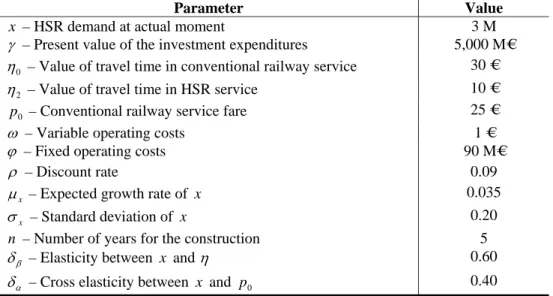
Table 1. Base-case parameters for the project
Parameter Value
x – HSR demand at actual moment 3 M
γ – Present value of the investment expenditures 5,000 M€
0
η – Value of travel time in conventional railway service 30 €
2
η – Value of travel time in HSR service 10 €
0
p – Conventional railway service fare 25 €
ω – Variable operating costs 1 €
ϕ – Fixed operating costs 90 M€
ρ – Discount rate 0.09
x
µ – Expected growth rate of x 0.035
x
σ – Standard deviation of x 0.20
n – Number of years for the construction 5
β
δ – Elasticity between x and η 0.60
α
δ – Cross elasticity between x and p0 0.40
Note: M = Millions
Table 2 presents the HSR line investment valuation results for the base-case parameters.
Table 2. Project valuation results
Output Value
∗
x – Critical demand for HSR service (n.º passengers) 10.777 M
( )
xv – Investment Opportunity Value 3,743.3 M€
npv – Net Present Value 254.2 M€
vod – Value of the Option do Defer 3,489.1 M€
Based on the results obtained, the construction of the HSR line should only start when the demand reaches 10,777 million passengers. Although the project registers a slightly positive NPV, it shouldn’t be implemented at the current time, concerning the uncertainty regarding the number of passengers of the new service. Maintaining “alive” this investment opportunity has a value of 3,743 million euros, of which 93,21% results from the value of the option to defer the investment.
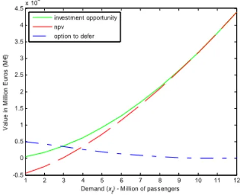
Figure 1 represents the evolution of the investment’s opportunity value, the NPV and the option to defer according to the demand xt increase throughout time. As we
may observe, if the demand exceeds 10,777 million passengers, the option to defer the implementation no longer has value. Thus, from this point on, the decision to immediately implement the project is the one which maximizes the value for its owners.
Figure 1. Investment’s opportunity value, NPV and value of the option to defer, for
the base case
1 2 3 4 5 6 7 8 9 10 11 12 -0.5 0 0.5 1 1.5 2 2.5 3 3.5 4 4.5x 10 4
Demand (xt) - Million of passengers
V a lu e in M illio n E u ro s ( M € ) investment opportunity npv option to defer
Figure 2 to Figure 7 show the sensibility of the valuation indicators of the project regarding the variation of some parameters.
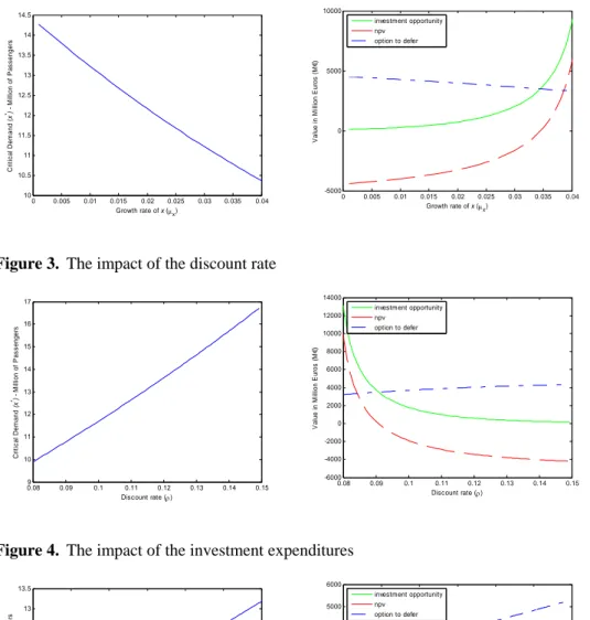
Figure 2. The impact of the growth rate 0 0.005 0.01 0.015 0.02 0.025 0.03 0.035 0.04 10 10.5 11 11.5 12 12.5 13 13.5 14 14.5 Growth rate of x (µx) C rit ic a l D e m a n d ( x *) - M ill io n of P a s s e nger s 0 0.005 0.01 0.015 0.02 0.025 0.03 0.035 0.04 -5000 0 5000 10000 Growth rate of x (µx) V a lue i n M il li on E u ro s ( M €) investment opportunity npv option to defer
Figure 3. The impact of the discount rate
0.089 0.09 0.1 0.11 0.12 0.13 0.14 0.15 10 11 12 13 14 15 16 17 Discount rate (ρ) Cr it ic al De m a n d (x *) - M il li on of P a s s e nger s 0.08 0.09 0.1 0.11 0.12 0.13 0.14 0.15 -6000 -4000 -2000 0 2000 4000 6000 8000 10000 12000 14000 Discount rate (ρ) V a lue i n M il li on E u ro s ( M €) investment opportunity npv option to defer
Figure 4. The impact of the investment expenditures
40009 4500 5000 5500 6000 6500 7000 9.5 10 10.5 11 11.5 12 12.5 13 13.5 Investment expenditures M€ (γ) C ri ti c al dem and (x *) M il li on of P a s s e n ger s 4000 4500 5000 5500 6000 6500 7000 -2000 -1000 0 1000 2000 3000 4000 5000 6000 Investment expenditures M€ (γ) V a lue i n M il li on E u ro s ( M €) investment opportunity npv option to defer
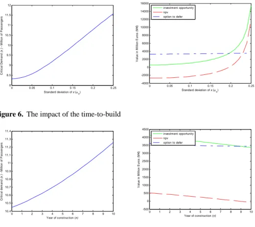
Figure 5. The impact of the volatility of the number of passengers 0 0.05 0.1 0.15 0.2 0.25 8 8.5 9 9.5 10 10.5 11 11.5 12 Standard deviation of x (σx) C rit ic a l D e m a n d (x *) - M il li o n of P a s s e nger s 0 0.05 0.1 0.15 0.2 0.25 -4000 -2000 0 2000 4000 6000 8000 10000 12000 14000 16000 Standard deviation of x (σx) V a lue i n M il li on E u ro s ( M €) investment opportunity npv option to defer
Figure 6. The impact of the time-to-build
0 1 2 3 4 5 6 7 8 9 10 10.4 10.5 10.6 10.7 10.8 10.9 11 11.1 11.2 11.3 11.4 Year of construction (n) C ri ti c al dem and (x *) - M il li on of P a s s e n ger s 0 1 2 3 4 5 6 7 8 9 10 -500 0 500 1000 1500 2000 2500 3000 3500 4000 4500 Year of construction (n) V a lue i n M il li on E u ro s ( M €) investment opportunity npv option to defer
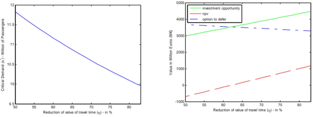
Thus, we may notice that critical demand level x∗ varies inversely with the demand growth rate µx (Figure 2) and with the reduction of the value of travel time given by
0 2 0 η η η −
which the HSR line enables (Figure 7). For higher demand growth rates µx and with major reductions in the value of travel time, the present value of the benefits resulting from the project increases, justifying anticipating its implementation.
The other parameters analyzed assume a direct relationship with the critical level of demand x∗. Larger discount rates (Figure 3), larger investment expenditures (Figure 4), larger volatility in the number of passengers (Figure 5) or more construction time needed (Figure 6) instigate significant postponements in the projects’ implementation.
Figure 7. The impact of the reduction in the value of travel time 50 55 60 65 70 75 80 9.5 10 10.5 11 11.5 12
Reduction of value of travel time (η) - in %
Cr it ic a l Dem and (x *) - M ill ion of P a s s enger s 50 55 60 65 70 75 80 -1000 0 1000 2000 3000 4000 5000
Reduction of value of travel time (η) - in %
V a lue i n M il li on E u ro s ( M €) investment opportunity npv option to defer
In presence of variations in any of the analyzed parameters, the investment’s opportunity value and the NPV always register the same trend, for each one of the parameters, although with different drifts. Figure 5 shows that NPV increases with uncertainty increase. This result originates from the fact that the valuation model incorporates the elasticity between HSR demand and the value of travel time and the cross elasticity between the HSR demand and the conventional service fare. This specificity of the developed model results in a value of the option to defer that slightly diminishes with the increase of uncertainty. These findings can also be seen in Figure 8. It is always assumed that the discount rate remains unchanged as the volatility of the project changes.
If a larger construction period of time is required, the increase in uncertainty throughout time and the delay of the benefits from the investment’s operation instigate a reduction in the investment’s opportunity value and in the NPV (Figure 6).
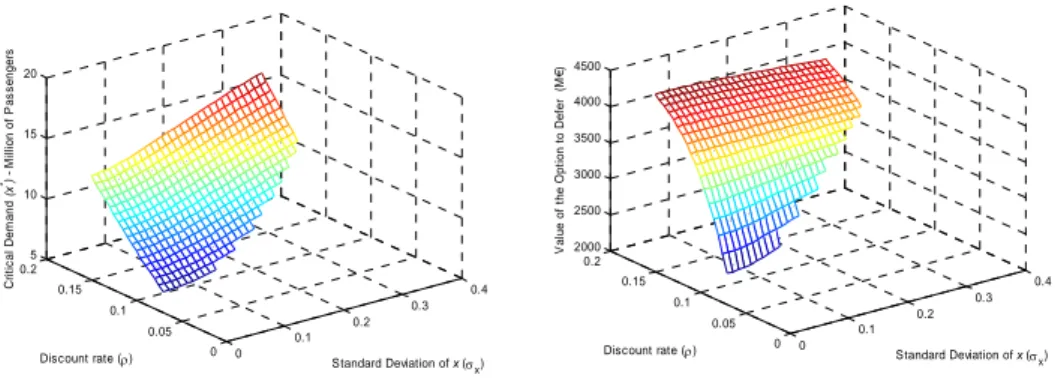
Figure 9 gives the joint impact of both the discount rate ρ and the investment expenditures γ in the critical demand value x∗ and in the value of the option to defer. Both valuation outputs shows a direct relationship with these two parameters, turning the option to defer more valuable as this project parameters value increase. As showed in Figure 3 and Figure 4 this is due to a deeper decrease in NPV than the one registered in the investment’s opportunity value.
Figure 8. The impact of both the volatility of the number of passengers and the discount rate 0 0.1 0.2 0.3 0.4 0 0.05 0.1 0.15 0.2 5 10 15 20 Standard Deviation of x (σx) Discount rate (ρ) Cr it ic a l Dem and (x *) - M illio n o f P a s s e n g e rs 0 0.1 0.2 0.3 0.4 0 0.05 0.1 0.15 0.2 2000 2500 3000 3500 4000 4500 Standard Deviation of x (σx) Discount rate (ρ) V a lue of t he O p ti on t o Def e r ( M € )
Figure 9. The impact of both the investment expenditures and the discount rate
4000 5000 6000 7000 0 0.05 0.1 0.15 0.2 5 10 15 20 25 Investment expenditures (γx) Discount rate (ρ) Cr it ic a l Dem and (x *) - M illio n o f P a s s e n g e rs 4000 5000 6000 7000 0 0.05 0.1 0.15 0.2 2000 3000 4000 5000 6000 7000 Investment expenditures (γx) Discount rate (ρ) V a lue of t h e O p ti on to Def e r ( M €)
5. Conclusion
The present work develops a model aimed at finding the optimal timing to implement a HSR investment, in an uncertain environment. We have introduced several adjustments to the original valuation model of the option to defer (McDonald and Siegel, 1986) and to the optimal stopping model of Salahaldin and Granger (2005), given the need to design a model applicable to an HSR investment in an environment of stochastic demand. As far has we are aware, the development of closed form solution ROA’s models to value railway investments was never done before.
The existence of a conventional railway service enables the analysis of the investment in HSR to be performed in an incremental basis, measured in terms of the corresponding utility functions. The indifference in the demand utility between HSR
and conventional railway services makes possible for the problem to be equated in terms of finding a critical demand level that justifies the project implementation.
The presented developments, regarding the optimal timing to invest and the investment’s opportunity value, have the advantage of offering a clear way to evaluate the utility of the HSR investment in each moment in time, for the set of potential users - the society in general. The numerical example and simulation of some important input parameters demonstrates the consistency of the model concerning the behaviour of the valuation outputs.
In future research, it should be possible to enrich the model in order to include more uncertainty sources – like the fare price and the investment expenditure. Additionally, we expect to perform an empirical application1 capable of providing the feedback useful to guide additional improvements in the structure of the modelling framework.
References
Bowe, M. and D. Lee (2004). Project Evaluation in the Presence of Multiple Embedded Real Options: Evidence From the Taiwan High-Speed Rail Project. Journal of Asian
Economics, 15, 71-98.
Brandão, L. (2002). Uma Aplicação da Teoria das Opções Reais em Tempo Discreto para Avaliação de uma Concessão Rodoviária no Brasil. PhD Thesis, PUC-Rio.
Copeland, T. and V. Antikarov (2003). Real Options: A Practitioner’s Guide. Thomson, Texere, New York.
Dixit, A. (1989). Entry and exit Decisions under Uncertainty. Journal of Political
Economy, 97 (3), 620-638.
Dixit, A.andR.Pindyck (1994). Investment Under Uncertainty. Princeton University Press, Princeton, New Jersey.
Majd, S. and R. Pindyck (1987). Time to Build, Option Value, and Investment Decisions. Journal of Financial Economics, 18 (1), 7-27.
Marathe, R and S. Ryan (2005). On the Validity of the Geometric Brownian Motion Assumption. The Engineering Economist, 50, 159-192.
McDonald, R. and D. Siegel (1986). The Value of Waiting to Invest. The Quarterly
Journal of Economics, 101 (4), 707-728.
1
Myers, S. (1977). Determinants of Capital Borrowing. Journal of Financial Economics, 5 (2), 147-175.
Nichols, N. (1994). Scientific Management at Merck: an Interview with CFO Judy Lewent. Harvard Business Review, January-February, 88-99.
Oksendal, B. (2003). Stochastic Differential Equations. An Introduction with Applications. Sixth Edition, Springer.
Owen, A. and G. Phillips (1987). The Characteristics of Railway Passengers Demand.
Journal of Transport Economics and Policy, 21, 231-253.
Paxson, D. and H. Pinto (2005). Rivalry Under Price and Quantity Uncertainty. Review
of Financial Economics, 14 (3-4), 209-224.
Pereira, P., A. Rodrigues and M. Armada (2006). The Optimal Timing for the Construction of an International Airport: a Real Options Approach with Multiple Stochastic Factors and Shocks. 10th Real Options Conference, New York.
Rose, S. (1998). Valuation of Interacting Real Options in a TollRoad Infrastructure Project. The Quarterly Review of Economics and Finance, 38, 711-723.
Ross, S. (1996). Stochastic Processes. Second Edition, Wiley Series in Probability and mathematical Statistics, John Wiley & Sons, Inc.
Salahaldin, L. and T. Granger (2005). Investing in Sustainable Transport to Relieve Air Pollution under Population-Growth Uncertainty. 9th Real Options Conference, Paris. Shilton, D. (1982). Modelling the Demand for High Speed Train Services. The Journal
of Operational Research Society, 33, 713-722.
Smit, H. (2003). Infrastructure Investment as Real Options Game: The Case of European Airport Expansion. Financial Management, 32 (4), 27-57.
Trigeorgis, L. (1996). Real Options: Managerial Flexibility and Strategy in Resource Allocation. The MIT Press, Cambridge, MA.
Wardman, M. (1994). Forecasting the Impact of Service Quality Changes on Demand for Inter-Urban Rail Travel. Journal of Transport Economics and Policy, 28, 287-306. Wardman, M. (1997). Inter-Urban Rail Demand, Elasticities and Competition in Great Britain: Evidence from Direct Demand Models. Transport Research E, 33 (1), 15-18. Wilson, G. (1986). Economic Analysis of Transportation: A Twenty-Five Year Survey.