Compressive Sensing Based Single-Pixel Imaging Systems

Single-Pixel Imaging Systems

Filipe Tiago Alves de Magalhães

Thesis submitted to the Faculty of Engineering in partial fulfillment of the requirements

for the degree of Doctor of Philosophy in Electrical and Computer Engineering

Work supervised by

Miguel Fernando Paiva Velhote Correia, PhD

Assistant Professor at the Department of Electrical and Computer Engineering

Faculdade de Engenharia da Universidade do Porto

and by

Francisco Manuel da Moita Araújo, PhD

Senior Researcher at the Optoelectronics and Electronic Systems Unit – UOSE

INESC TEC

The candidate has been financially supported by the FCT - Fundação para a Ciência e a Tecnologia (Portuguese Foundation for Science and Technology) through a Ph.D. grant.

“Estudar é uma coisa em que está indistinta A distinção entre nada e coisa nenhuma.” in Liberdade, Fernando Pessoa

“Study's the thing where the distinction Is unclear between nothing and nothing at all.” in Liberty, Fernando Pessoa

I would like to address my special thanks to Prof. Miguel Velhote for having accepted this challenge and for all the guidance provided and availability demonstrated in all our interactions. I am sure this relationship has just been the start of something even greater.

I would like to express my very great appreciation to Dr. Francisco Araújo who since the beginning of this thesis showed an impressive encompassing perspective. After so many years of collaboration, it was extremely fulfilling to reach this point with him by my side.

I am also particularly grateful to Prof. Faramarz Farahi for welcoming me in his lab and even at his home and for providing me the opportunity to work and learn on such a friendly, creative and enthusiastic environment. It has been a pleasure to become a link of the already existing chain, between these two sides of the Atlantic, which spreads far beyond science and technology.

To Mehrdad Abolbashari I must say that his patience and never ending availability have been much esteemed. Thank you for all the interesting and productive discussions we had and for all the contributions. I really enjoyed the time we spent together, not only on a scientific perspective but also on a personal level. I hope we can continue to collaborate in the future.

Thank you to all those that have helped me to solve those “little big” issues, in particular to Nuno Sousa and Eduardo Marques, for the help with the electronics and with the C++ programming for the LightCommander, respectively.

To Dr. Rui Martins from the Centre of Molecular and Environmental Biology at the University of Minho I would like to say that I much appreciated the enthusiasm with which he got involved with my work and the help he gave me in finding applications for it.

To Ricardo Sousa I would like to acknowledge the cooperation we established and the help provided with the machine learning mechanisms.

I am thankful to Rita Pacheco for the help provided in clarifying the doubts related with the English language.

I would like to recognize the encouragement and support provided by Prof. Aurélio Campilho to the creation and establishment of the BioStar group.

X

I have to say to Hélder Oliveira that it has been a pleasure to be his partner during these last four years and that the BioStar has been a very enjoyable adventure.

To Marco Scipioni I would like to say thank you for sharing with me his keen curiosity and for bringing up many meaningful “small” questions. I must also recognize that the occasions we spent together, be it talking about Physics, doing sports or just having a laugh, surely were pleasant.

Many thanks to the UOSE team at INESC TEC for granting me with the adequate conditions and resources despite the setbacks we found along the way. Thank you for believing in me and for the excellent working atmosphere.

I would like to acknowledge the Fundação para a Ciência e a Tecnologia (FCT) for the financial support given through the form of a PhD grant. I also kindly thank the Fundação Luso-Americana para o Desenvolvimento (FLAD) and the Fundação Calouste Gulbenkian for the funding provided for travelling expenses.

I was also very fortunate to have my friends and family always caring about me.

To my aunt Alice, for all her love and dedication, I would like to say that she will be forever in my heart.

To my parents, for being a source of endless love and support, I would like to express my deepest gratitude. Without them I would surely not be who and where I am today.

Domo arigatō gozaimashita Joana for all your love and all the good things we have together. I will always be by your side…

It would be unfair trying to refer all those that have made a difference throughout these years because they were so many and I would end up forgetting someone, but as “no man is an island”, here I leave a word of recognition for them.

Compressive sensing has recently emerged and is now a subject of increasing research and discussion, undergoing significant advances at an incredible pace. The novel theory of compressive sensing provides a fundamentally new approach to data acquisition which overcomes the common wisdom of information theory, specifically that provided by the Shannon-Nyquist sampling theorem. Perhaps surprisingly, it predicts that certain signals or images can be accurately, and sometimes even exactly, recovered from what was previously believed to be highly incomplete data.

In 2006, the Digital Signal Processing group at Rice University created a single-pixel camera, which fused an innovative camera hardware architecture with the mathematical theory and algorithms of compressive sensing. This work constituted the start sparkle for the development of many enthusiastic and impressive compressive imaging systems, which now define state-of-the-art solutions in many imaging applications.

In this thesis, initially, a comprehensive review of the current state-of-the-art of compressive imaging systems with particular emphasis in single-pixel architectures is presented. Afterwards, the main subject of this thesis is explored and the single-pixel imaging systems which were developed for various imaging modalities are exposed, namely for monochrome, color, multispectral, hyperspectral and high dynamic range imaging. For each of these modalities a configuration that operated with passive illumination and another that operated with active illumination has been implemented. This allowed a thorough comparative analysis to be made. An algorithm was also developed and demonstrated for the generation of compressive random binary codes to be used by a CMOS imager and enrich it with a compressive imaging mode of operation.

There was still the opportunity to explore the developed compressive single-pixel imaging systems in three different applications. In one of those applications, a passive illumination single-pixel monochrome imaging system has been mounted on a microscope and has been used to acquire images with very fine spatial resolution. In another application, the theory of compressive sensing has been combined with machine learning and pattern recognition mechanisms to detect faces without explicit image reconstruction. Within this context, the passive illumination single-pixel monochrome imaging system has also been used to acquire real-world data and test this innovative concept. The third application used a passive illumination single-pixel hyperspectral imaging system to derive spectroscopic information of grapes from hyperspectral images. This information may be used to analyze and assess the physicochemical properties of the grapes.

Before the concluding remarks, a tangible idea is presented for future consideration. It is related with the development of a compressive single-pixel imaging LIDAR system for the aerospace industry.

A sensorização compressiva surgiu recentemente e constitui hoje um assunto de grande investigação e discussão, manifestando avanços significativos com uma cadência impressionante. A inovadora teoria de sensorização compressiva fornece-nos uma abordagem fundamentalmente nova ao tema da aquisição de dados que ultrapassa o conhecimento comum providenciado pela teoria da informação, em particular aquele estabelecido pelo teorema da amostragem de Shannon-Nyquist. Talvez surpreendentemente, ela prevê que certos sinais ou imagens podem ser recuperados com precisão, e por vezes de um modo exacto, a partir do que anteriormente se acreditava serem dados altamente incompletos.

Em 2006, o Digital Signal Processing Group da Universidade de Rice criou uma câmara com um único pixel, que fundiu uma arquitectura inovadora de hardware com a teoria matemática e os algoritmos da sensorização compressiva. Este trabalho foi determinante para o desenvolvimento entusiástico e impressionante de muitos sistemas de imagiologia compressiva que definem actualmente soluções ao nível do estado-da-arte em diversas aplicações.

Nesta tese, inicialmente, é apresentada uma revisão extensa do estado-da-arte actual no que respeita a sistemas de imagiologia compressivos com particular ênfase nas arquitecturas que empregam um único pixel. Depois, o tema principal desta tese é explorado e são expostos os sistemas de imagiologia com um único pixel que foram desenvolvidos para diferentes modalidades, nomeadamente para aquisição de imagens monocromáticas, a cores, multiespectrais, hiperespectrais e de gama dinâmica alargada. Para cada uma das modalidades foi implementada uma configuração que operava com iluminação passiva e outra que operava com iluminação activa. Isto permitiu realizar uma análise comparativa minuciosa dos sistemas em causa. Foi também desenvolvido e demonstrado um algoritmo de geração dos códigos compressivos para ser usado por um sensor de imagem CMOS e enriquecê-lo com um modo compressivo de aquisição de imagens.

Houve ainda a oportunidade de explorar os sistemas desenvolvidos em três aplicações. Numa dessas aplicações, um sistema de iluminação passiva para aquisição de imagens monocromáticas com um único pixel foi montado num microscópio e foram obtidas imagens com uma resolução espacial muito fina. Noutra aplicação, a teoria de sensorização compressiva foi combinada com mecanismos de aprendizagem computacional para detecção de faces sem a reconstrução explícita das imagens. Neste contexto, o sistema de iluminação passiva para aquisição de imagens monocromáticas com um único pixel foi usado para adquirir dados reais e testar este conceito inovador. A terceira aplicação usou um sistema de iluminação passiva para aquisição de imagens hiperespectrais com um único pixel para derivar informação espectroscópica de uvas. Esta informação pode ser usada para analisar e avaliar as suas propriedades físico-químicas. Antes das notas finais, é apresentada uma ideia para prossecução futura relacionada com o desenvolvimento de um sistema LIDAR de imagiologia com um único pixel para a indústria aeroespacial.

Acknowledgements ... IX Abstract ... XI Resumo ... XIII List of Figures ... XVII List of Tables ... XXXIII List of Acronyms ... XXXV Chapter 1. Introduction ... 1 1.1 Thesis structure ... 3 1.2 Motivation ... 3 1.3 Contributions ... 4 1.4 Publications ... 6

Chapter 2. The Theory of Compressive Sensing – An Overview... 7

2.1 K-sparse and compressible signals ... 7

2.2 Recovering K-sparse signals... 8

2.3 Incoherence ... 8

2.4 How compressive sensing works... 9

2.5 Robustness of compressive sensing ... 12

Chapter 3. Compressive Imaging Systems – A Review ... 15

3.1 The single-pixel camera ... 15

3.2 Feature-specific structured imaging system ... 17

3.3 Random projections based feature-specific structured imaging ... 18

3.4 Compressed sensing magnetic resonance imaging ... 19

3.5 Single-pixel terahertz imager ... 22

3.6 Compressive structured light for recovering inhomogeneous participating media ... 26

3.7 Compressive spectral imagers ... 27

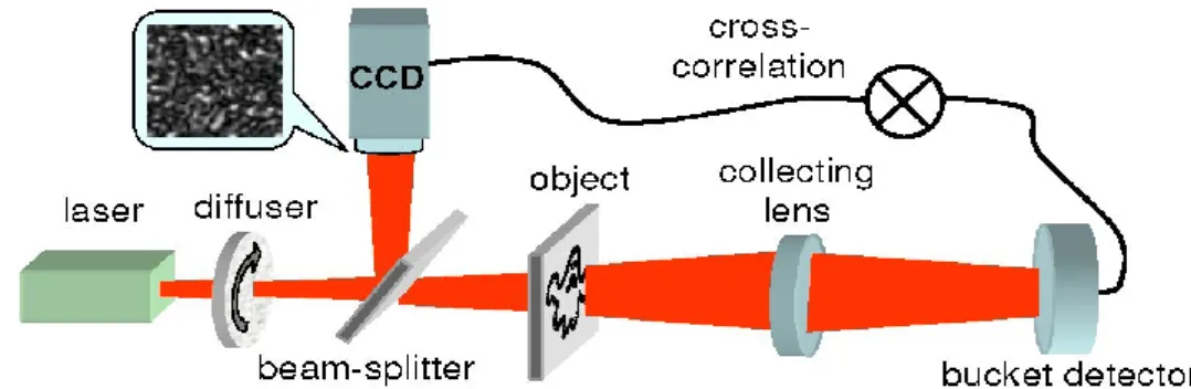
3.8 Compressive ghost imaging system ... 34

3.9 CMOS compressive sensing imager ... 36

3.10 Compressive microscopy imaging systems ... 38

3.11 Compressive optical coherence tomography ... 41

3.12 Photon-counting compressive sensing laser radar for 3D imaging ... 45

3.13 Millimeter-wave imaging with compressive sensing ... 47

3.14 Compressive polarimetric imaging ... 50

Chapter 4. Compressive Sensing Based Single-Pixel Imaging Systems ...53

4.1 Monochrome Imaging Systems ... 53

4.1.1 Active illumination single-pixel monochrome imaging system ... 53

XVI

4.1.3 Transmissive single-pixel imaging system ... 79

4.1.4 Concluding remarks ... 85

4.2 Color Imaging Systems ... 87

4.2.1 Active illumination single-pixel color imaging systems ... 87

4.2.2 Passive illumination single-pixel color imaging systems ... 97

4.2.3 Concluding remarks ... 101

4.3 Multispectral Imaging Systems ... 103

4.3.1 Active illumination single-pixel multispectral imaging system ... 103

4.3.2 Passive illumination multispectral single-pixel imaging system ... 109

4.3.3 Concluding remarks ... 112

4.4 Hyperspectral Imaging Systems ... 113

4.4.1 Active illumination single-pixel hyperspectral imaging system ... 114

4.4.2 Passive illumination single-pixel hyperspectral imaging system ... 119

4.4.3 Concluding remarks ... 132

4.5 High Dynamic Range Compressive Imaging Systems ... 133

4.5.1 Active illumination high dynamic range compressive imaging system ... 142

4.5.2 Passive illumination high dynamic range compressive imaging system ... 149

4.5.3 Concluding remarks ... 156

4.6 CMOS Based Compressive Imaging Sensor ... 157

4.6.1 Overall architecture and operation ... 157

4.6.2 Compressive sensing based mode of operation ... 159

4.6.3 Concluding remarks ... 161

Chapter 5. Applications ... 163

5.1 Microscopic imaging using a passive illumination single-pixel monochrome imaging system ... 163

5.2 Face detection without explicit image reconstruction ... 164

5.3 Physicochemical analysis of grapes based on hyperspectral images ... 173

Chapter 6. Future Work ... 181

6.1 Single-Pixel Imaging LIDAR System Based on Compressive Sensing ... 181

Chapter 7. General Conclusions... 185

Figure 1 – Example of a simple recovery problem. (a) The Logan–Shepp phantom test image. (b) Sampling domain in the frequency plane; Fourier coefficients are sampled along 22 approximately radial lines. (c) Minimum energy reconstruction obtained by setting unobserved Fourier coefficients to zero. (d) Compressive sensing based reconstruction. This reconstruction is an exact replica of the original image in (a) [5]. ... 2 Figure 2 – Geometry of



1 recovery. (a) Visualization of the



2 minimization that finds the

non-sparse point of contact

sˆ

between the



2 ball (hypersphere, in red) and the translated measurement matrix null space (in green). (b) Visualization of the



1 minimization solution that finds the sparse point of contact

sˆ

with high probability thanks to the pointiness of the



1 ball. Picture adapted from [19]. ...11 Figure 3 – Single-Pixel Camera block-diagram. Incident light field (corresponding to the desired image x ) is reflected off a DMD array whose mirror orientations are modulated by a pseudorandom pattern. Each different mirror pattern produces a voltage at the single photodiode that corresponds to one measurement

y

 

m

. From M measurements a

sparse approximation to the desired image x using CS techniques can be obtained. Picture reproduced from [15]...15 Figure 4 – Optical setup of the single-pixel camera developed at the Rice University. Picture reproduced from [15]. ...16 Figure 5 – Flow diagram for the Feature-Specific Structured Imaging (FSSI) system. Picture reproduced from [31]. ...17 Figure 6 – Flow diagram for the binary Random Projections FSSI (RPFSSI) system. Picture reproduced from [32]. ...19 Figure 7 – Scheme of a CS based MRI system. The user controls the gradient waveforms and RF pulses (block (a)) that, in turn, control the phase of the pixels/voxels (block (b)) in the image. An RF coil receives the signal in an encoded form (block (c)). The incoherent measurements result from the control of the gradient waveforms (block (d)). An image can then be reconstructed with an appropriate nonlinear reconstruction enforcing sparsity (block (e)). Picture reproduced from [36]. ...20

XVIII

Figure 8 – 3D contrast enhanced angiography. Even acquiring only 10% of the samples, CS could recover most of the blood vessel information revealed by Nyquist sampling and significantly reduce the artifacts when compared to the linear reconstruction. Images taken from [36]. ... 21 Figure 9 – Brain scanning using MRI. The results obtained with CS, using fewer sampling trajectories, were comparable to those obtained with the full Nyquist-sampled set. CS was also more successful than linear reconstruction from incoherent sampling in suppressing aliasing artifacts and exhibited improved resolution over a low-resolution acquisition with the same scan time. Picture reproduced from [36]. ... 22 Figure 10 – CS-based THz Fourier imaging setup. Picture reproduced from [37]. ... 23 Figure 11 – Compressive sensing imaging results. (a) Magnitude of image reconstructed by inverse Fourier transform using the full dataset (4096 uniformly sampled measurements) and (d) its phase. Note the phase distortion inherent in the THz beam in (d). Compressed sensing reconstruction result using 500 measurements (12%) from the full dataset: (b) magnitude and (e) phase. Compressed sensing with phase correction improves image quality (c) and eliminates phase distortion (f). All figures show a zoom-in view on a 40



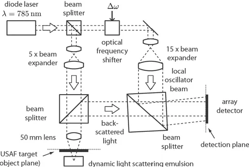
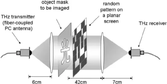
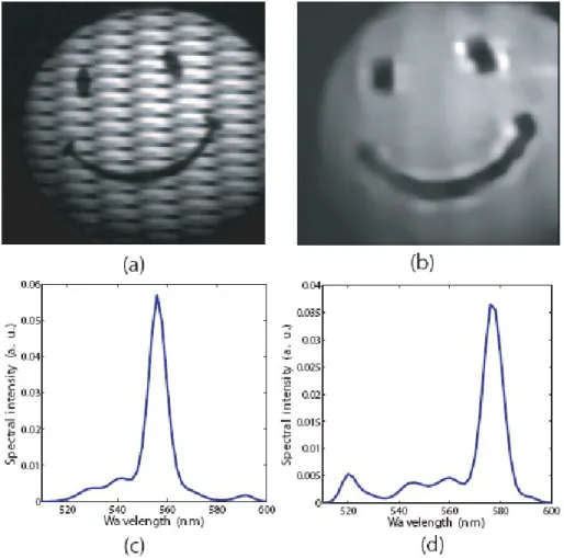
_{40 grid centered on the object. Picture reproduced from [37]. ... 24} Figure 12 – Diagram of the CS-based THz imaging system discarding the need for raster scanning. Picture reproduced from [38]. ... 25 Figure 13 – Compressive structured light for recovering inhomogeneous participating media. (a) Coded light is emitted along the z-axis to the volume while the camera acquires images as line-integrated measurements of the volume density along the x-axis. The light is coded in either the spatial domain or temporal domain with a predetermined sequence. (b) Image formation model for participating medium under single scattering. The image irradiance at one pixel, I(y, z), depends on the integral along the x-axis of the projector‟s light, L(x, y), and the medium density, ρ(x, y, z), along a ray through the camera center. (c) Experimental setup. The volume density is reconstructed from the measurements by the use of compressive sensing techniques. Picture reproduced from [39]. ... 26 Figure 14 – Reconstruction results of milk drops dissolving in water. 24 images were used to reconstruct the volume at 128 × 128 × 250 at 15fps. The reconstructed volumes are shown in three different views and the image in the leftmost column shows the corresponding photograph (taken with all projector pixels emitting white) of the dynamic process). Picture reproduced from [39]. ... 27 Figure 15 – Schematic drawing of the single-shot CS-based spectral imager. Picture reproduced from [40]. ... 27

image recorded for illumination with a 10 nm full width at half maximum (FWHM) bandpass filter centered at 560 nm – note the modulation introduced by the coding aperture. (b) Intensity image generated by summing the spectral information in the reconstruction for the 560 nm bandpass filter. (c) Spectral reconstruction at a particular spatial location for the 560 nm bandpass filter. (d) Spectral reconstruction at a particular spatial location for the 580 nm bandpass filter. The small peak near 520 nm is due to spectral aliasing. Picture and info reproduced from [40]. ...29 Figure 18 – Schematic drawing of the SD-CASSI system. Picture reproduced from [41]. ...30 Figure 19 – Top view of the SD-CASSI experimental setup. Picture reproduced from [41]. ...30 Figure 20 – Scene consisting of a ping-pong ball illuminated by a 543 nm green laser and a white light source filtered by a 560 nm narrowband filter (left), and a red ping-pong ball illuminated by a white light source (right). Picture reproduced from [41]. ...31 Figure 21 – Spatial content of the scene of Figure 20 in each of 28 spectral channels between 540 and 640 nm. The green ball can be seen in channels 3 to 8; the red ball can be seen in channels 23 to 25. Picture reproduced from [41]. ...31 Figure 22 – (left) Spectral intensity through a point on the ping-pong ball illuminated by a 543 nm green laser and a white light source filtered by a 560 nm narrowband filter. (right) Spectral intensity through a point on the red ping-pong ball illuminated by a white light source. Spectra from an Ocean Optics non-imaging reference spectrometer are shown for comparison. Picture reproduced from [41]. ...32 Figure 23 – (a) Mosaic of hyperspectral images with a lateral resolution of 256 x 256 pixels and a spectrum resolution of 4 nm (averaged over several channels). (b) Reconstructed image after summing all the bands. (c) Image taken with a conventional camera. Images reproduced from [42]. ...33 Figure 24 – 256 x 256 pixels images for two spectral bands obtained via raster scan (left column) and compressive sensing (right column). Images reproduced from [42]. ...34 Figure 25 – Scheme of a standard setup for pseudothermal ghost imaging with two detectors. Picture reproduced from [43]...35 Figure 26 – Scheme of the compressive ghost imaging setup with a single detector. Picture reproduced from [43]. ...35

XX

Figure 27 – Ghost imaging results for the reconstruction of images of a double-slit transmission plate. Top row: Conventional ghost imaging with: (a) 256 realizations; (b) 512 realizations; Bottom row: Compressive ghost imaging reconstruction using the same experimental data as in (a) and (b). Picture reproduced from [43]. ... 36 Figure 28 – Scheme of the CMOS CS-imager. Picture reproduced from [45]. ... 38 Figure 29 – Schematic drawing of the compressive confocal microscope along with its principle of operation. Picture reproduced from [48]. ... 39 Figure 30 – Diagram of the experimental off-axis, frequency-shifting digital holography setup. Picture reproduced from [51]. ... 40 Figure 31 – (a) Results obtained with standard holography. (b) CS reconstruction, using 7% of the Fresnel coefficients. Images reproduced from [51]. ... 41 Figure 32 – Scheme of the common path spectral domain OCT setup. Picture reproduced from [53]. ... 42 Figure 33 – OCT image of onion cells: (a) obtained using complete spectral data; (b), (c), and (d) obtained by sampling 62.5%, 50%, 37.5% of the pixels and pursuing sparsity in pixel domain; (e), (f), and (g) obtained by sampling 62.5%, 50%, 37.5% of the pixels and pursuing sparsity in wavelet domain. Picture reproduced from [53]. ... 43 Figure 34 – Setup of the swept-source OCT system constructed with a 1060 nm source and a standard Michelson interferometer. The regular raster scan pattern was modified to acquire randomly spaced horizontal B-scans. The full volume was generated through CS-recovery in post processing. Picture reproduced from [54]. ... 44 Figure 35 – Results recovered with CS. The top row shows the position of the frames that were acquired, the second row shows the CS reconstructed summed voxel projection, the third and fourth row show a selected B-scan and slow scan from the CS-recovered info, respectively. Picture reproduced from [54]... 45 Figure 36 – Experimental setup of the photon-counting compressive sensing laser radar system for 3D imaging. Picture reproduced from [13]. ... 46 Figure 37 – Results obtained with the photon-counting compressive sensing laser radar system for 3D imaging. Reconstructions for objects „U‟ and „R‟ at depths 1.75 m and 2.10 m. (a) and (b) consider only „U‟ and „R‟, respectively, while (c) considers a range including both. Timing histogram (d) peaks represent, from left to right, „U‟, „R‟, and the room wall. Picture reproduced from [13]. ... 46

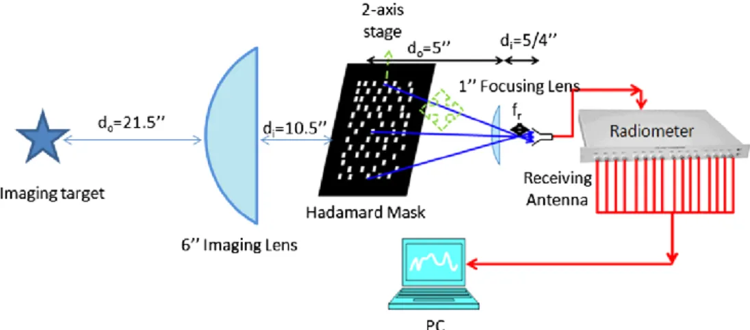
acquisitions. Picture reproduced from [62]. ...48 Figure 39 – Diagram of the compressive sensing based passive mm-wave imaging setup. Picture reproduced from [63]. ...49 Figure 40 – 41 × 43 pixels images of the incandescent bulb acquired with the CS based PMMW system with: (a) 100% and (b) 11% of the samples. Picture reproduced from [63]. ...49 Figure 41 – Setup for single-pixel imaging polarimetry. An example of a binary intensity pattern displayed by the SLM is also shown. Picture reproduced from [64]. ...50 Figure 42 – (a) 1024 × 1024 pixels image of the object used in the experiment, which consists of an amplitude mask with a cellophane film covering the zone colored in yellow. (b), (c) and (d) represent 64 × 64 pixels pseudo-color images for the Stokes parameters. Picture reproduced from [64]. ...51 Figure 43 – Active illumination single-pixel-camera experimental setup. Following the red arrows, it can be seen that the image projected by the video projector is reflected on the wall and by means of a lens is focused on the photodiode active area. The output of the photodiode amplifier circuit is connected to a data acquisition board. ...54 Figure 44 – (a) Compact active illumination single-pixel camera setup. (b) Detailed photo of the assembly comprising the lens and the photodiode circuit. ...55 Figure 45 – Schematics of the photodiode amplifier circuit...55 Figure 46 – Example of one of the projected images, representing the product between a random measurement pattern and the image to be reconstructed. ...56 Figure 47 – (a) Reference image. First results obtained (32×32 pixels  N = 1024) with the active illumination single-pixel camera using: (b) 205 measurements  20% (PSNR = 11.08 dB); (c) 410 measurements  40% (PSNR = 12.30 dB); (d) 717 measurements 

70% (PSNR = 13.21 dB). All the PSNR were calculated using the reference image and the respective reconstructed image. ...56 Figure 48 – (a) Original scene; Image reconstruction using: (b) 20% of the measurements (PSNR = 69.74 dB); (c) 40% of the measurements (PSNR = 75.60 dB); (d) 60% of the measurements. All the reconstructions are images with 64 × 64 pixels (N = 4096). All the PSNR values were obtained comparing the respective image with the image reconstructed using 60% of the measurements. ...57

XXII

Figure 49 – Reconstruction of the image of Figure 47 c) after the addition of uniformly distributed noise with maximum amplitude of: (a) 10% of the maximum amplitude of the measured signal (SNR = 20.63 dB) – PSNR = 26.62 dB; (b) 20% of the maximum amplitude of the measured signal (SNR = 14.54 dB) – PSNR = 25.03 dB; (c) 30% of the maximum amplitude of the measured signal (SNR = 11.41 dB) – PSNR = 20.17 dB; (d) 40% of the maximum amplitude of the measured signal (SNR = 8.48 dB) – PSNR = 13.87 dB. All the PSNR values were calculated comparing the respective image with the image of Figure 47 c). ... 58 Figure 50 – Spectral responsivity of the Thorlabs PDA100A-EC amplified Silicon photodiode. Picture reproduced from the manual, available at http://thorlabs.com/Thorcat/13000/PDA100A-Manual.pdf. ... 59 Figure 51 – Scheme of the compressive active illumination single-pixel imaging system. ... 61 Figure 52 – Photo of the compressive active illumination single-pixel imaging system. ... 61 Figure 53 – Photo of the black and white wood object with character “A” taken with a conventional camera. ... 62 Figure 54 – Several images of the black and white wood object containing the character “A”. Image resolution (in pixels) from top to bottom: 32 × 32; 64 × 64; 128 × 128; 512 × 512. Left column contains the images acquired with the active illumination single-pixel monochrome imaging system. Center column contains the images represented in left column after median filtering and contrast adjustment. Right column contains the images acquired with a conventional camera downsized for comparison purposes. ... 63 Figure 55 – Plot of the voltage signal on the output of the amplified photodiode circuit. It is clearly seen the effect of the variable modulation and ripple of the light. ... 64 Figure 56 – Five-pointed black star filled with three different gray levels. ... 67 Figure 57 – Several images of the grayscale five-pointed star. Image resolution (in pixels) from top to bottom: 32 × 32; 64 × 64; 128 × 128. Left column contains the images obtained with the active illumination single-pixel monochrome imaging system. Center column contains the images represented in left column after median filtering and contrast adjustment. Right column contains the images acquired with a conventional camera downsized for comparison purposes. ... 68 Figure 58 – Photos of the LightCommander™ development kit from Logic PD. ... 70 Figure 59 – LightCommander‟s optical schematics. (Kindly provided by LogicPD) ... 71

http://de.academic.ru/pictures/dewiki/68/DLP_Chip.jpg. ...71 Figure 61 – (a) Schematic of two mirrors from a digital micromirror device (DMD), illustrating its principle of operation. (b) A portion of an actual DMD array with an ant leg for scale. Picture reproduced from [23]...72 Figure 62 – Scheme of the passive illumination single-pixel monochrome imaging system. ...73 Figure 63 – Photo of the passive illumination single-pixel monochrome imaging system illuminating the black and white wood object of Figure 53. ...73 Figure 64 – (left) Several images of the black and white wood object containing the character “A” acquired with the passive illumination single-pixel monochrome imaging system. (right) Images acquired with a conventional camera downsized for comparison purposes. ...74 Figure 65 – (left) Several images of the grayscale five-pointed star acquired with the passive illumination single-pixel monochrome imaging system. (right) Images acquired with a conventional camera downsized for comparison purposes. ...76 Figure 66 – Illustration for the definition of a projector‟s throw ratio. ...79 Figure 67 – Scheme of the transmissive single-pixel imaging system. ...80 Figure 68 – Transmissive single-pixel camera mounted on a microscope, placed on the vertical optical path. Note the conventional camera (in blue) mounted on the other optical path. ...81 Figure 69 – Photo of the LCD module taken from the Epson® PowerLite S5 projector that has been used in the transmissive single-pixel camera (active area: 11.2 mm × 8.4 mm). ...81 Figure 70 – Thorlabs FDS series photodiode responsivity curves. The yellow curve relates to the photodiode (FDS1010) used on the transmissive single-pixel camera setup. Picture reproduced from http://www.thorlabs.de/Thorcat/2700/2739-s01.pdf...82 Figure 71 – Image of one of the acquired scenes. This image was obtained from the stitching of 4 separate pictures taken with the conventional camera due to its sensor size (1/2-inch CCD) when compared to the size of the LCD active region. The red inset indicates the region acquired with our single-pixel camera. ...82 Figure 72 – Reconstruction of an image with 32 × 32 pixels (N= 1024) from: (a) 25% (K_{= 256);}

(b) 50% (K_{= 512); (c) 75% (}K_{= 768); (d) 100% (}K_{= 1024) measurements. For each}

reconstructed image, the PSNR has been calculated relatively to the image reconstructed using 100% (K= 1024) of the measurements: (a) PSNR = 12.85 dB; (b)

XXIV

Figure 73 – Reconstruction of an image with 64 × 64 pixels (N= 4096) from: (a) 25% (K_{= 1024);}

(b) 50% (K_{= 2048); (c) 75% (}K_{= 3072); (d) 100% (}K_{= 4096) measurements. For each}

reconstructed image, the PSNR has been calculated relatively to the image reconstructed using 100% (K _{= 4096) of the measurements: (a) PSNR = 20.27 dB; (b)}

PSNR = 22.63 dB; (c) PSNR = 32.44 dB. ... 83 Figure 74 – Halogen lamp emission spectrum, obtained with a commercial spectrometer. ... 85 Figure 75 – (a) Piece of paper with the painted red contour and green background (the coin is present only for size comparison). (b) Color image of the painted area in (a), reconstructed with 32 × 32 pixels (410 measurements were acquired for each of the RGB channels). ... 88 Figure 76 – Color reconstruction of a 64 × 64 pixels image of the real scene depicted in Figure 48 (a). 40% of the measurements were used to reconstruct each image associated with the RGB channels. ... 88 Figure 77 – Photo of the colored wood object with character “B”. ... 89 Figure 78 – Photo with detail of the colored wood object being illuminated with a green and black random binary compressive measurement code with 32 × 32 pixels. ... 89 Figure 79 – Spectra of the RGB components used for illumination along with the spectrum of the “white” light resulting from their combinations. ... 90 Figure 80 – Illustrative examples of the application of the post-processing algorithm (selective local median filter) and median filtering to filter noisy points. The white portion of the matrix with a thicker black border represents the 3 × 3 neighborhood under analysis. ... 91 Figure 81 – Images of the colored wood object containing the character “B” acquired with the active illumination color imaging system with spectral filtering on the illumination end. Image resolution (in pixels) from top to bottom: 32 × 32; 64 × 64; 128 × 128. (left) Color images filtered with the selective local median filter. (center) Color images after median filtering. (right) Images acquired with a conventional camera downsized for comparison purposes. ... 92 Figure 82 – Spectra of the RGB components resulting from filtering the “white” light emitted by the projector. ... 94

Image resolution (in pixels) from top to bottom: 32 × 32; 64 × 64; 128 × 128. (left) Color images filtered with the selective local median filter. (center) Color images after median filtering. (right) Images acquired with a conventional camera downsized for comparison purposes. ...95 Figure 84 – 128 x 128 pixels image obtained after median filtering the raw images representative of the RGB channels. ...95 Figure 85 – From left to right, images representative of the Red, Green and Blue components with 128 × 128 pixels. ...96 Figure 86 – Images of the colored wood object containing the character “B” acquired with the passive illumination color imaging system with spectral filtering on the illumination end. Image resolution (in pixels) from top to bottom: 32 × 32; 64 × 64; 128 × 128. (left) Color images filtered with the selective local median filter. (center) Color images after median filtering. (right) Images acquired with a conventional camera downsized for comparison purposes. ...98 Figure 87 – Images of the colored wood object containing the character “B” acquired with the passive illumination color imaging system with spectral filtering on the detection end. Image resolution (in pixels) from top to bottom: 32 × 32; 64 × 64; 128 × 128. (left) Color images filtered with the selective local median filter. (center) Color images after median filtering. (right) Images acquired with a conventional camera downsized for comparison purposes. ... 100 Figure 88 – Scheme of the setup for the active illumination single-pixel multispectral imaging system. ... 103 Figure 89 – Normalized emission spectra of the red, green and blue LED light bulbs used for illumination in the active illumination single-pixel multispectral imaging system. ... 104 Figure 90 – Photos of the active illumination single-pixel multispectral imaging system. Left: Light from the blue LED light bulb is being launched into the Lightcommander‟s tunnel. The LightCommander‟s illumination module and respective power unit have been removed. Right: Detailed photo of the amplified photodiode and of the scene being illuminated with a binary random code. ... 104 Figure 91 – RGB scene composed to be used on the performance evaluation of the active illumination single-pixel multispectral imaging system. ... 105

XXVI

Figure 92 – From top to bottom: 32 × 32; 64 × 64; 128 × 128; pixels images captured with the active illumination single-pixel multispectral imaging system. The RGB images resulting from the combination of the raw images after selective local median filtering can be seen on the left column, while the center column contains the RGB images resulting from the combination of the raw images after median filtering. On the right column, it can be seen the images acquired with a conventional camera downsized for comparison purposes. ... 106 Figure 93 – 128 × 128 pixels images acquired to evaluate the reflectance of the printed scene of Figure 91. On the top row it can be seen the images acquired with the active illumination single-pixel multispectral imaging system after median filtering. The photos acquired with a conventional camera are displayed on the bottom row. The images represented from left to right, illustrate the acquisitions made when the scene was being independently illuminated with the red, green, and blue LED bulb, respectively. ... 108 Figure 94 – Plot of the normalized voltage on the output of the amplified photodiode circuit when one LED light bulb was being used for illumination of the scene being acquired. ... 109 Figure 95 – Scheme of the setup for the passive illumination single-pixel multispectral imaging system. ... 110 Figure 96 – Photo of the passive illumination single-pixel multispectral imaging system during operation. ... 110 Figure 97 – From top to bottom: 32 × 32, 64 × 64 and 128 × 128 pixels images captured with the passive illumination single-pixel multispectral imaging system. On the left column are the RGB images obtained after filtering each color channel raw image with the selective local median filter. The center column contains the RGB images obtained after median filtering each color channel raw image. On the right column, it can be seen images acquired with a conventional camera downsized for comparison purposes. ... 111 Figure 98 – Setup of the active illumination single-pixel hyperspectral imaging system. ... 115 Figure 99 – Photo of the active illumination single-pixel hyperspectral imaging system. ... 115 Figure 100 – Paper with “V” and “E” characters printed in black in a red and green background, respectively. ... 116 Figure 101 – Images with different resolutions obtained with the active illumination single-pixel hyperspectral imaging system for the paper object with the characters “V” and “E” printed in black in a red and green background, respectively (see Figure 100). The images on the left column were obtained when the He-Ne laser (red) was on and the images on the right column were obtained when the Nd:YAG laser (green) was on. .. 117

camera when the scene was being illuminated with the He-Ne laser (on the left) or with the Nd:YAG laser (on the right). These photos have been resized to 128 × 60 pixels for comparison with the images displayed in Figure 102... 118 Figure 104 – RGB image resulting from the addition of the images of Figure 102. ... 118 Figure 105 – Reflectance spectra of the red and green regions of the scene presented in Figure 100. In black it is also presented the emission spectrum of the halogen bulb that was used for illumination. ... 119 Figure 106 – Photo of the Infocus LP120 video projector. ... 120 Figure 107 – Scheme depicting the principle of operation of the Zollner-Thurnar's type monochromator of the ANDO AQ6317B optical spectrum analyser (OSA). ... 121 Figure 108 – Scheme depicting the principle of operation of the passive illumination single-pixel hyperspectral imaging system. ... 122 Figure 109 – Optical engine of the Infocus LP120 projector. ... 123 Figure 110 – Detailed photo of the Infocus LP120 with the 10x microscope objective launching the light into the 50/125 µm multi-mode optical fiber. ... 123 Figure 111 – Normalized reconstructed spectrum obtained along the reconstructed datacube in a fixed spatial position where the laser line was imaged (black trace). The red trace represents the normalized spectrum of the He-Ne source measured with the OSA. .. 124 Figure 112 – Rows (a) and (c) represent the images reconstructed at 632.800 nm with 32 × 32 and 64 × 64 pixels, respectively, along with a 3-D representation of their normalized intensities. Rows (b) and (d) represent the images reconstructed at 632.790 nm with 32 × 32 and 64 × 64 pixels, respectively, along with a 3-D representation of their normalized intensities. ... 125 Figure 113 – Detailed photo of the assembly used for launching light coming from LightCommander‟s light tunnel into the optical fiber. ... 126 Figure 114 – 512 × 512 pixels photo of the lit LED lamp acquired with: (a) conventional camera; (b) with passive illumination single-pixel hyperspectral camera, at 630.900 nm. ... 126 Figure 115 – PSNR versus the percentage of measurements used to reconstruct the 512 × 512 pixels images of the lit LED bulb with respect to their full dimensionality. All the PSNR values were calculated relatively to the 512 × 512 pixels image reconstructed using 100% of the measurements [see Figure 114 (b)]. ... 127

XXVIII

Figure 116 – Photo of an Ocean Optics USB 2000 miniature fiber optic spectrometer. Image reproduced from http://www.oceanoptics.com/Products/usb2000.asp. ... 129 Figure 117 – (left) Ocean Optics USB 2000 miniature fiber optic spectrometer without the cover. (right) Scheme of the light path through the optical arrangement of the USB2000. The

photo on left was reproduced from

http://www.biophotonicsworld.org/system/uploads/0000/0037/IMG_9538.JPG. .. 129 Figure 118 – Conventional camera photo of the composed scene of a red LED bulb being hit by a spot of a laser emitting at 654 nm. ... 131 Figure 119 – Spectrum of the scene composed by a red LED bulb and by a laser spot at 654 nm. The spectrum directly measured with the USB 2000 spectrometer is represented in black while the spectrum obtained along the reconstructed datacube is represented in red... 131 Figure 120 – 128 × 128 pixels images reconstructed at 630.88 nm and 654.03 nm, representing the red LED bulb and the laser spot, respectively. ... 132 Figure 121 – Picture of a hemispherical surface... 135 Figure 122 – Example of a sinusoidal fringe pattern used for the extraction of 3D information about the object into which it is projected. ... 135 Figure 123 – Photos of the hemispherical object from Figure 121 with a sinusoidal pattern projected on its surface, acquired with a conventional camera using different exposure times and gains: (a) exposure time: 31 ms, gain: 14; (b) exposure time: 230 ms, gain: 81. ... 136 Figure 124 – Scheme of the experimental setup used for high dynamic range imaging with adaptive intensity control. ... 137 Figure 125 – Photo of the experimental setup used for high dynamic range imaging with adaptive intensity control. ... 137 Figure 126 – Flowchart of the application developed for adaptive intensity control. ... 138 Figure 127 – Results obtained with the adaptive intensity control imaging system for the acquisition of high dynamic range images of a hemispherical surface (top row) and of a metallic and highly reflective object (bottom row): (a) and (d) initial image; (b) and (e) final image; (c) and (f) mask applied to the LCD that provided the acquisition of the final image. ... 139 Figure 128 – Synthetic scene created to evaluate the performance of the HDRCI system. ... 140 Figure 129 – Photos of the scene depicted in Figure 128, acquired with a conventional camera, using different exposure times: (a) 1/320 s; (b) 1/25 s. ... 141

Figure 131 – Flowchart describing the procedure for HDRCI by means of acquiring images with different equivalent exposure times. ... 143 Figure 132 – Photo of the active illumination HDRCI system under operation. ... 143 Figure 133 – 128 × 128 pixels image initially obtained with low equivalent exposure time and without mask, using the active illumination HDRCI system. ... 144 Figure 134 – 128 × 128 pixels image obtained with equivalent long exposure time and with a mask totally blocking the right half part, using the active illumination HDRCI system. ... 144 Figure 135 – 128 × 128 pixels high dynamic range image resulting from the combination of the images acquired with different equivalent exposure times of Figure 133 and Figure 134. Tone mapping has been used to display the image with 8 bits. ... 145 Figure 136 – Flowchart of the algorithm implemented for HDRCI by means of intensity control. ... 146 Figure 137 – (a) 128 × 128 pixels image reconstructed with the active illumination HDRCI system when the mask displayed in (b) was used. The mask reduced 60% the radiance of the right half of scene. ... 147 Figure 138 – 128 × 128 pixels high dynamic range image resulting from the division of the image in Figure 137 (a) by the mask displayed in Figure 137 (b). Tone mapping has been used to display the image with 8 bits. ... 148 Figure 139 – Normalized intensity measured by the photodiode as a function of the gray level [0, 255] of the image projected with the Epson® video projector... 149 Figure 140 – Scheme of the passive illumination HDRCI system. ... 149 Figure 141 – Top view photo of the passive illumination HDRCI system. ... 150 Figure 142 – General view of the passive illumination HDRCI system during operation. Next to the lower right corner of the photo, it is possible to see the amplified photodiode mounted in front of the LightCommander light tunnel. ... 151 Figure 143 – 128 × 128 pixels image initially obtained with low equivalent exposure time and without mask, using the passive illumination HDRCI system. ... 151 Figure 144 – 128 × 128 pixels image obtained with equivalent long exposure time and with a mask totally blocking the right half part, using the passive illumination HDRCI system. ... 152

XXX

Figure 145 – 128 × 128 pixels high dynamic range image resulting from the combination of the images acquired with different equivalent exposure times of Figure 143 and Figure 144. Tone mapping has been used to display the image with 8 bits. ... 152 Figure 146 – (a) 128 × 128 pixels image reconstructed with the passive illumination HDRCI system when the mask displayed in (b) was used. The mask reduced 50% the radiance of the right half of scene. ... 153 Figure 147 – 128 × 128 pixels high dynamic range image resulting from the division of the image in Figure 146 (a) by the mask displayed in Figure 146 (b). Tone mapping has been used to display the image with 8 bits. ... 153 Figure 148 – Binary PWM sequence pattern with two examples of how intensity values are generated with 5 bits. ... 154 Figure 149 – Plots of the measured PWM signals when different gray levels were being assigned to the DMD pixels. ... 155 Figure 150 – Normalized intensity measured by the photodiode as a function of the gray level [0, 255] of the image projected with the LightCommander. ... 156 Figure 151 – Architecture of the CMOS based imaging sensor. ... 158 Figure 152 – Layout of the integrated circuit of the imaging sensor. ... 159 Figure 153 – 32 × 32 pixels image with several geometric shapes and different gray levels used in the simulations performed to study the feasibility of the algorithm created to generate binary random compressive codes to be used by the CMOS based imaging sensor. .... 161 Figure 154 – 32 × 32 pixels reconstructions of the image in Figure 153. The reconstructions were performed using: (a) 10% (PSNR = 5.32 dB); (b) 50% (PSNR = 12.51 dB), of the total number of measurements (1024). The PSNR were calculated relatively to the image of Figure 153. ... 161 Figure 155 – Photo of the LightCommander with the photodiode in front of the light tunnel assembled on a Leica microscope. ... 164 Figure 156 – 128 × 128 pixels result images acquired with: (left) the compressive single-pixel imaging system; (right) a conventional camera; assembled on the microscope, for a scene consisting of the characters “ste” printed in black on standard white paper. ... 164 Figure 157 – Examples of images belonging to the created sets. (Top) Images of faces of three persons in upright frontal positions, with two examples for the same person. (Bottom) Images of three different objects/animals, with two examples for the same object. .... 165

Figure 159 – Three different standard approaches for feature selection: (left) depicts the filter feature selection (FS) approach done before the model design (MD); (center) the wrapper consists on an iterative approach where features are removed step by step until a desirable performance of the model is achieved; and (right) embedded method is designed jointly with the learning model algorithm. ... 167 Figure 160 – Performance of the SVM classifier trained with different amounts of data and with random feature selection... 167 Figure 161 – Performance of the SVM classifier trained with different amounts of data and with optimized feature selection. ... 168 Figure 162 – Examples of images belonging to the created sets with over imposed blobs representing the SIFT descriptors. ... 169 Figure 163 – Photo of the arrangement used to acquire the measurements for face detection with the passive illumination single-pixel imaging system. ... 170 Figure 164 – Images of a face (128 × 128 pixels) and of an object (256 × 256 pixels) that have been used to assess the performance of the face detection system under real-world conditions with the passive illumination single-pixel monochrome imaging system. ... 170 Figure 165 – Images of Figure 164 resized to 32 × 32 pixels. ... 171 Figure 166 – Images of a face (PSNR = 12.41 dB) and of an object (PSNR = 9.86 dB) with 32 × 32 pixels reconstructed using 1024 measurements acquired with the passive illumination single-pixel monochrome imaging system. The PSNR values were calculated using the homologous images of Figure 165 as references. ... 171 Figure 167 – Images of a face (PSNR = 24.84 dB) and of an object (PSNR = 22.93 dB) with 32 × 32 pixels reconstructed using 1024 measurements obtained multiplying the image to be reconstructed by the Hadamard random binary codes. The PSNR values were calculated using the homologous images of Figure 165 as references. ... 172 Figure 168 – Setup used to acquire hyperspectral images of grapes with the passive illumination single-pixel hyperspectral imaging system. ... 174 Figure 169 – Photos of the three grapes with different maturation levels illuminated in transmission. These photos were acquired with a conventional camera. From left to right, the grapes had 13.7 %Bx, 16.8 %Bx and 20.8 %Bx. ... 174

XXXII

Figure 170 – (left) 32 × 32 pixels image of the grape with 20.8 %Bx acquired at 671.02 nm with the passive illumination hyperspectral imaging system. (right) The seeds observable in the image on the left were highlighted with a red contour. ... 175 Figure 171 – 32 × 32 pixels image of the halogen bulb behind the opening on the black plastic piece at 645.10 nm acquired with the passive illumination hyperspectral imaging system. ... 175 Figure 172 – 32 × 32 pixels image of the halogen bulb with three points marked in red, green and blue to indicate the positions where the spectra were obtained along the datacube. .... 176 Figure 173 – Spectra obtained along the halogen bulb datacube in the positions marked by the red, green and blue pixels in the image of Figure 172. ... 176 Figure 174 – Spectra of the halogen bulb. The normalized real spectrum is represented with a thick black trace while the normalized integrated spectrum, obtained from the reconstructed datacube, is represented with a thin red trace. ... 177 Figure 175 – Transmission spectra obtained from the datacube of the grape with 20.8 %Bx in the positions marked by the red, green and blue pixels in the image of Figure 172. ... 178 Figure 176 – Transmission spectra of the grape with 20.8 %Bx. The normalized real spectrum is represented with a thick black trace while the normalized integrated spectrum, obtained from the reconstructed datacube, is represented with a thin red trace. ... 179 Figure 177 – Normalized integrated transmission spectra of the three grapes, obtained from each of the respective datacubes. ... 179 Figure 178 – Scheme illustrating the principle of operation of the single-pixel imaging LIDAR system based on compressive sensing. ... 182

List of Tables

Table 1 – Comparison between the number of measurements required by the RPFSSI and FSSI systems to achieve the same RMSE-based performance...19 Table 2 – Comparison of the main aspects of DD-CASSI and SD-CASSI. ...32 Table 3 – Equipment for the active illumination single-pixel imaging system. ...60 Table 4 – PSNR values obtained for the reconstructed images of Figure 54 relatively to the images acquired with the conventional camera. ...65 Table 5 – Maximum values of the normalized cross-correlation obtained for the reconstructed images of Figure 54 relatively to the images acquired with the conventional camera. ....66 Table 6 – Time taken to perform 100% of the measurements needed to reconstruct the images with different resolutions, using the Epson® video projector to project the compressive codes. ...67 Table 7 – Time consumed during reconstruction for different compression levels and different resolutions. ...67 Table 8 – PSNR values obtained for the reconstructed images of Figure 57 relatively to the images acquired with the conventional camera. ...69 Table 9 – Maximum values of the normalized cross-correlation obtained for the reconstructed images of Figure 57 relatively to the images acquired with the conventional camera. ....69 Table 10 – Main specifications of the Nikon lens that accompanies the LightCommander. ...71 Table 11 – PSNR values obtained for the reconstructed images of Figure 64 relatively to the images acquired with the conventional camera. ...75 Table 12 – Maximum values of the normalized cross-correlation obtained for the reconstructed images of Figure 64 relatively to the images acquired with the conventional camera. ....75 Table 13 – PSNR values obtained for the reconstructed images of Figure 65 relatively to the images acquired with the conventional camera. ...76 Table 14 – Maximum values of the normalized cross-correlation obtained for the reconstructed images of Figure 65 relatively to the images acquired with the conventional camera. ....77 Table 15 – Time taken to perform 100% of the measurements needed to reconstruct the images with different resolutions, using the Lightcommander‟s to project the compressive codes. ...78

XXXIV

Table 16 – PSNR values obtained for the reconstructed images of Figure 81 relatively to the images acquired with the conventional camera. ... 93 Table 17 – Maximum values of the normalized cross-correlation obtained for the reconstructed images of Figure 81 relatively to the images acquired with the conventional camera. .... 93 Table 18 – PSNR values obtained for the reconstructed images of Figure 83 relatively to the images acquired with the conventional camera. ... 96 Table 19 – Maximum values of the normalized cross-correlation obtained for the reconstructed images of Figure 83 relatively to the images acquired with the conventional camera. .... 96 Table 20 – PSNR values obtained for the reconstructed images of Figure 86 relatively to the images acquired with the conventional camera. ... 99 Table 21 – Maximum values of the normalized cross-correlation obtained for the reconstructed images of Figure 86 relatively to the images acquired with the conventional camera. .... 99 Table 22 – PSNR values obtained for the reconstructed images of Figure 87 relatively to the images acquired with the conventional camera. ... 101 Table 23 – Maximum values of the normalized cross-correlation obtained for the reconstructed images of Figure 87 relatively to the images acquired with the conventional camera. .. 101 Table 24 – PSNR values obtained for the reconstructed images of Figure 92 relatively to the images acquired with the conventional camera. ... 107 Table 25 – Maximum values of the normalized cross-correlation obtained for the reconstructed images of Figure 92 relatively to the images acquired with the conventional camera. .. 107 Table 26 – PSNR values obtained for the reconstructed images of Figure 97 relatively to the images acquired with the conventional camera. ... 112 Table 27 – Maximum values of the normalized cross-correlation obtained for the reconstructed images of Figure 97 relatively to the images acquired with the conventional camera. .. 112 Table 28 – Noise equivalent power and maximum noise current for the PDA100A amplified photodiode when the gain of 50 dB or 60 dB was chosen. ... 147

List of Acronyms

1D – One-Dimensional 2D – Two-Dimensional 3D – Three-Dimensional APD – Avalanche PhotoDiode CCD – Charge-Coupled Device CI – Computational Imaging

CMOS – Complementary Metal Oxide Semiconductor CS – Compressive Sensing

DLP – Digital Light Processing DMD – Digital Micromirror Device DWT – Discrete Wavelet Transform FOV – Field Of View

FWHM – Full Width at Half Maximum HDR – High Dynamic Range

HDRI – High Dynamic Range Imaging

HDRCI – High Dynamic Range Compressive Imaging He-Ne – Helium-Neon

HSI – HyperSpectral Imaging ILS – Imaging LIDAR System JPEG – Joint Picture Experts Group LCD – Liquid Crystal Display

LC-SLM – Liquid Crystal Spatial Light Modulator LED – Light Emitting Diode

LIDAR – LIght Detection And Ranging

MOEMS – Micro-Opto-Electro-Mechanical Systems MP3 – Moving Picture Experts Group Layer-3 Audio MRI – Magnetic Resonance Imaging

XXXVI

MSE – Mean-Square-Error

Nd:YAG – Neodymium Yttrium Aluminum Garnet OCT – Optical Coherence Tomography

Pixel – Picture (Pix) + Element PMMW – Passive MilliMeter-Wave PSNR – Peak Signal-to-Noise Ratio PWM – Pulse-Width Modulation QE – Quantum Efficiency

RGB – Red – Green – Blue color space RIP – Restricted Isometry Principle RMSE – Root-Mean-Square Error SLM – Spatial Light Modulator SNR – Signal-to-Noise Ratio SVM – Support Vector Machine THz – TeraHertz

Chapter 1. Introduction

It is clear that the Nyquist-Shannon sampling theorem has been a fundamental rule of signal processing for many years and can be found in nearly all signal acquisition protocols, being extensively used from consumer video and audio electronics to medical imaging devices or communication systems. Basically, it states that a band-limited input signal can be recovered without distortion if it is sampled at a rate of at least twice the bandwidth of the signal. For some signals, such as images that are not naturally band limited, the sampling rate is dictated not by the Nyquist-Shannon theorem but by the desired temporal or spatial resolution. However, it is common in such systems to use an anti-aliasing low-pass filter to band limit the signal before sampling it, and so the Nyquist-Shannon theorem plays an implicit role [1].

In the last few years, an alternative theory has emerged, showing that super-resolved signals and images can be reconstructed from far fewer data or measurements than what is usually considered necessary. This is the main concept of compressive sensing (CS), also known as compressed sensing, compressive sampling and sparse sampling. In fact, “the theory was so revolutionary when it was created a few years ago that an early paper outlining it was initially rejected on the basis that its claims appeared impossible to substantiate [2].”

CS relies on the empirical observation that many types of signals or images can be well approximated by a sparse expansion in terms of a suitable basis, that is, by only a small number of non-zero coefficients. This is the key aspect of many lossy compression techniques such as JPEG (Joint Picture Experts Group) and MP3 (Moving Picture Experts Group Layer-3 Audio), where compression is achieved by simply storing only the largest basis coefficients of a sparsifying transform.

In CS, since the number of samples taken is smaller than the number of coefficients in the full image or signal, converting the information back to the intended domain would involve solving an underdetermined matrix equation. Thus, there would be a huge number of candidate solutions and, as a result, a strategy to select the “best” solution must be found.

Different approaches to recover information from incomplete data sets have existed for several decades. One of its earliest applications was related with reflection seismology, in which a sparse reflection function (indicating meaningful changes between surface layers) was sought from band limited data [1, 3, 4]. It was, however, very recently, that the field has gained increasing attention, when Emmanuel J. Candès, Justin Romberg and Terence Tao [5], discovered that it was possible to reconstruct Magnetic Resonance Imaging (MRI) images from what appeared to be highly incomplete data sets in face of the Nyquist-Shannon criterion (see Figure 1). Following Candès et al. work , this decoding or reconstruction problem can be seen as an optimization problem and be efficiently solved using the 1-norm [6] or the total-variation [7, 8].

Compressive Sensing Based Single-Pixel Imaging Systems

2

Figure 1 – Example of a simple recovery problem. (a) The Logan–Shepp phantom test image. (b) Sampling domain in the frequency plane; Fourier coefficients are sampled along 22 approximately radial lines. (c) Minimum energy reconstruction obtained by setting unobserved Fourier coefficients to zero. (d) Compressive sensing based reconstruction. This reconstruction is an exact replica of the original image in (a) [5].

As a result, CS has become a kind of revolutionary research topic that draws from diverse fields, such as mathematics, engineering, signal processing, probability and statistics, convex optimization, random matrix theory and computer science.

Undergoing significant advances, CS has proved to be far reaching and has enabled several applications in many fields, such as: distributed source coding in sensor networks [9, 10], coding, analog–digital (A/D) conversion, remote wireless sensing [1, 11], 3D LIDAR [12, 13] and inverse problems, such as those presented by MRI [14].

One application with particular interest within the aim of the work presented here, is the ground-breaking single-pixel imaging setup developed by D. Takhar et al. at the Rice University [15]. This camera represented a simple, compact and low cost solution that could operate efficiently across a much broader spectral range than conventional silicon based cameras.

1.1 Thesis structure

This thesis is divided in seven chapters as follows:

 Chapter 1 presents the motivation and structure of the thesis. The main contributions and a record of publications are also enumerated.

 Chapter 2 describes the mathematical background of compressive sensing theory along with its main properties;

 Chapter 3 reviews the evolution of compressive sensing based imaging systems;  Chapter 4 expounds the core work of this thesis. It describes the experimental work

and results associated with the development of compressive single-pixel imaging systems for different imaging modalities. An algorithm that can concede a compressive sensing based operation mode to a CMOS imager is also presented.  Chapter 5 exemplifies distinct applications for two of the compressive single-pixel

imaging systems described in Chapter 4.

 Chapter 6 exposes one prospective idea for future pursuance aiming the reinforcement and exploitation of the competencies inherited from the work presented in this thesis.

 Chapter 7 closes the thesis with some concluding remarks.

1.2 Motivation

In a technological era where commercial cameras have reached tens of Megapixels, the theory of compressive sensing has emerged as a new paradigm which has been particularly materialized in the form of single-pixel cameras that operate, at least on a first look, in a counter intuitive manner.

Based on compressive sensing, single-pixel cameras can reconstruct images from fewer data than what is usually considered necessary. This creates the potential to perform faster still ensuring the quality of the results. Additionally, with these cameras, the information is gathered in an encrypted form right from the moment it is acquired, therefore bringing advantages in terms of storage/transmission and security. Their principle of operation places most of the complexity on the decoding end, which typically possesses more resources and can be improved disregarding the subtleties of the data acquired and provide even better reconstruction results with the same data.

Because of their versatility different light detection devices may be used, which brings benefits in terms of sensitivity and signal quality. Furthermore, these cameras created opportunities to operate with increased spectral resolution in wavelengths that were practically impossible or very expensive before.

Compressive Sensing Based Single-Pixel Imaging Systems

4

From a personal point of view, despite the particularly exploratory nature of the subject, it was with great pleasure and enthusiasm that I have embraced it. It constituted an opportunity to further extend my knowledge and to work in such a revolutionary and novel theme as that of compressive sensing. Having in mind the risks and implications of such decision, the initially posed challenge has been turned into an extremely rewarding experience that will certainly contribute to my personal and professional future as well as to the future of the research group.

1.3 Contributions

At an institutional level it should be said that the work presented in this thesis stimulated the establishment of a new research and actuation area inside the Optoelectronics and Electronic Systems Unit at INESC TEC. Besides the direct benefits this aspect raised in terms of innovation and creation of knowledge, it also helped to reinforce the privileged position INESC TEC has been setting for long in the scientific community. In concrete terms, new cooperation opportunities have been initiated with the European Space Agency; with universities from different countries, namely, the University of North Carolina at Charlotte (USA); the University of Minho (Portugal); the University Jaume I (Spain), and with industrial partners, to explore applications of the knowledge gathered with this work.

Concerning the theme of this thesis the following main contributions can be enumerated. Several different compressive single-pixel imaging systems have been developed, methodically characterized and compared. These systems were capable of acquiring monochrome, color, multispectral, hyperspectral and high dynamic range images, operating either in a passive or in an active illumination mode.

Emphasis should be directed towards the implemented active illumination single-pixel monochrome imaging system, which was the first to present a compressive sensing based principle of operation and that enabled the subsequent development of active illumination compressive single-pixel imaging systems for different modalities (color, multispectral, hyperspectral and high dynamic range).

A high dynamic range imaging system using an LCD for the spatial control of the image intensity was implemented. The knowledge gathered with this system would later be used for the development of an innovative high dynamic range compressive imaging technique, as will be exposed further below in this text.

A transmissive compressive single-pixel imaging system has also been developed and used to acquire microscopic images. To the extent of our knowledge, we were the first to present an imaging system that used an LCD to incorporate the compressive random binary codes into the system and produce the incoherent projections characteristic of compressive imaging. The development of this system has given us an adequate insight to compare LCD with DMD as spatial light modulators for compressive single-pixel cameras.