Equity Valuation Using Accounting Numbers in
High and Low Price to Performance Firms
António Carlos Vidal de Beça Pereira
4
thSeptember 2014
Dissertation submitted in partial fulfilment of requirements for the degree of MSc in Business Administration at the Universidade Católica Portuguesa,
4th September 2014. ! ! ! ! ! !
Equity Valuation Using Accounting Numbers in High and Low
Intangible-Intensive Industries
Rita Albuquerque Silva (152110043)
Advisor: Ricardo Ferreira Reis
!
!
Dissertation submitted in partial fulfilment of requirements for the degree of MSc in Business
Abstract
The surge of new industries in the economy has made commonplace a situation where firms are trading at prices greatly superior to their financial performance. In such conditions doubts may arise regarding the use of traditional valuation models to estimate the value of high price to performance firms.
This dissertation has as its main goal to determine if there is a variation in terms of performance by traditional valuation models when applied to high and low price to performance firms. Furthermore, the representation of performance by an accounting number is also studied in order to determine if such classification results in significant differences across firms.
It is found that when price to operating income before depreciation (P/OI) is used to separate firms into high and low P/OI sub-‐samples more significant differences between sub-‐samples arise than when price to net income (P/NI) is used. Moreover, valuation models are found to be less biased and more accurate, although explaining price worse, when applied to high P/OI firms. Finally, relevant differences are discovered regarding the use of nonfinancial information to represent firm performance by analysts and firms.
Key Words: Operating Income, Operating Income Before Depreciation (OIBDP),
Net Income (NI), P/OI, P/NI, Residual Income Model (RIM), Price-‐Earnings Multiple (P/E), Valuation Errors
Table of Contents
Chapter 1: Introduction ... 4
1.1 Motivation ... 4
1.2 Defining Operating Performance and a High/Low Price to Operating Performance Firm ... 4
1.3 Outline ... 5
Chapter 2: Literature Review ... 6
2.1 Introduction and Basic Concepts ... 6
2.2 Accounting-‐Based Valuation Models ... 7
2.2.1 Multiples-‐Based Models ... 7
2.2.1.1 Selecting the Value Driver ... 8
2.2.1.2 Selecting Comparable Firms ... 8
2.2.1.3 Computing the Benchmark Multiple ... 9
2.2.2 Flows-‐Based Valuation Models ... 10
2.2.2.1 Discounted Dividend Model (DIV) ... 10
2.2.2.2 Discounted Cash-‐Flow Model (DCF) ... 11
2.2.2.3 Residual Income Model (RIM) ... 11
2.2.2.3.1 Residual Income Model (RIM) Implementation Issues ... 13
2.2.2.4 Abnormal Earnings Growth Model (AEGM) ... 14
2.2.3 Conclusion on the Accounting-‐Based Valuation Models ... 15
2.3 Concluding Remarks on the Literature Review ... 15
Chapter 3: Large Sample Analysis ... 17
3.1 Introduction ... 17
3.1.1 Aim, Scope and Structure of the Large Sample Analysis ... 17
3.1.2 Hypotheses Development ... 17
3.2 Research Design ... 18
3.2.1 Sample Selection ... 18
3.2.2 Data and Variable Definitions ... 19
3.2.3 Research Methods ... 21
3.2.3.1 Residual Income Model (RIM) ... 21
3.2.3.2 Price to Earnings Multiple (P/E) ... 22
3.2.3.3 Performance Measures ... 22
3.3 Descriptive Statistics ... 23
3.3.1 General Descriptive Statistics ... 23
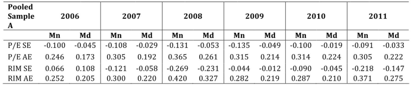
3.3.2 Descriptive Statistics by Fiscal Year ... 25
3.4 Data Analysis ... 26
3.4.1 Signed and Absolute Valuation Errors ... 26
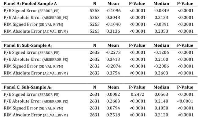
3.4.1.1 Descriptive Statistics ... 26
3.4.1.1.1 General Descriptive Statistics ... 26
3.4.1.1.2 Descriptive Statistics by Fiscal Year and SIC3 ... 27
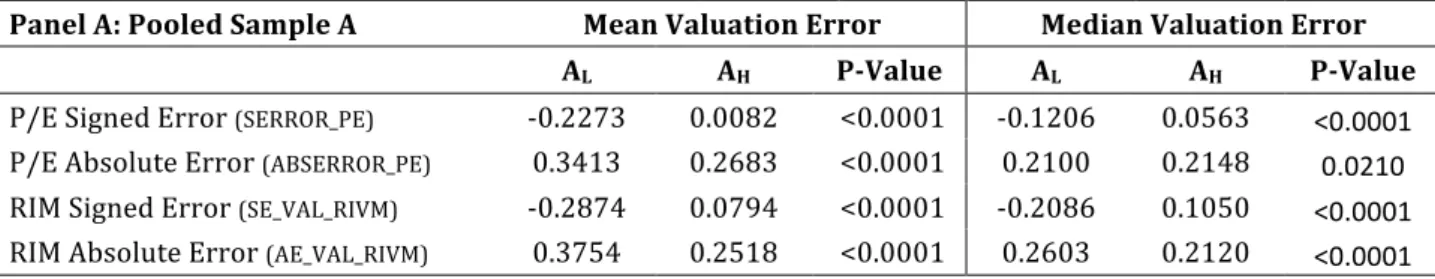
3.4.1.2 Statistical Tests ... 28
3.4.1.2.1 Test on the Accuracy and Bias of Valuation Models ... 28
3.4.1.2.2 Test on the Equality of Accuracy and Bias Across Sub-‐Samples ... 29
3.4.1.2.2 Test on the Equality of Accuracy and Bias Across Valuation Models ... 30
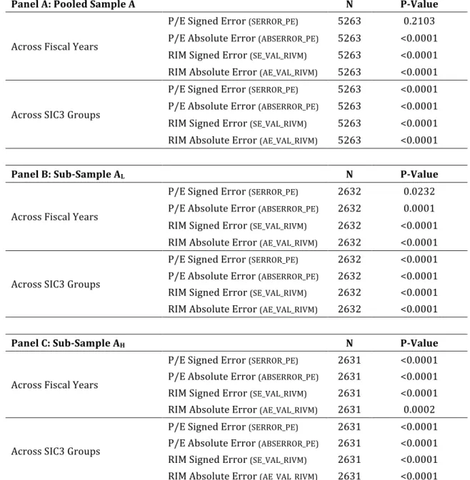
3.4.1.2.3 Equality of Value Estimates Across Fiscal Years and SIC3 Groups ... 31
3.4.2 Explanatory Power of Valuation Models ... 32
3.5 Concluding Remarks on the Large Sample Analysis ... 33
Chapter 4: Small Sample Analysis ... 36
4.1.1 Aim, Scope and Structure of the Small Sample Analysis ... 36
4.1.2 Hypotheses Development ... 36
4.2 Sample Selection Process ... 37
4.3 Data Analysis ... 38
4.3.1 Dominant Valuation Models ... 38
4.3.2 Investment Recommendations ... 40
4.3.3 Forecast Horizons ... 42
4.4 Supplementary Analysis ... 43
4.4.1 Influence of Nonfinancial Information ... 43
4.4.1.1 Nonfinancial Information in Analyst Reports’ First Page ... 43
4.4.1.2 Nonfinancial Information in Annual Reports ... 45
4.4.2 Analyst Coverage ... 47
4.4.3 Firm Size ... 48
4.5 Concluding Remarks on the Small Sample Analysis ... 49
Chapter 5: Conclusion ... 51
6. References ... 52
Chapter 1: Introduction
1.1 Motivation
The growth and expansion of the digital economy has paved the way for firms that are highly valued even though their operating performance may be distant from their market value.
Trueman et al. (2000) remembered an analyst whose analysis on Amazon.com could justify any valuation between $1-‐$200 by changing assumptions at a time the company was trading at $130.
Although more than a decade has passed, the situation persists alongside the premise that Internet stocks are difficult to value (Trueman et al., 2000). This problem is most notable when looking at firms not publicly traded: for instance start-‐ups going through funding rounds or IPOs (Kim and Ritter, 1999).
Nonetheless, a parallel could be drawn with publicly traded firms to state that traditional valuation models perform worse on firms with high price relative to operating performance (P/OP) than on their counterparts that lie in the low end of this ratio.
It is interesting to study if this is a sound claim, given the current market size of companies such as Yahoo and, more recently, Facebook and Twitter -‐ firms that once were1 or still are included in this category and questioned2 on the
reasonability of their market prices.
1.2 Defining Operating Performance and a High/Low Price to Operating Performance Firm
Operating or operational performance are expressions used interchangeably throughout this dissertation. They designate key financials that lock-‐in a firm’s yearly business functioning in a figure, summing up the level of success achieved for the period.
To illustrate high P/OP firms Trueman et al. (2000) used P/E and Price-‐to-‐ Revenue. Similarly, in this dissertation operating performance will be represented in the large sample analysis by Operating Income Before Depreciation and in the small sample analysis by Net Income. The use of two
1 See, for example, Schonfeld, E., 2000. How Much Are Your Eyeballs Worth. Fortune, [online]. Available at:
<http://archive.fortune.com/magazines/fortune/fortune_archive/2000/02/21/273860/index.htm> [Accessed 2 August 2014].
2 See, for example, Berman, K., 2013. Is Twitter Really Worth $10 Billion?. The Wall Street Journal, [online].
Available at:
<http://online.wsj.com/news/articles/SB10001424127887323384604578328303487784818> [Accessed 2 August 2014].
different proxies will allow for a representation of operating performance firstly as the business proper and secondly as the overall success of the firm.
1.3 Outline
This dissertation will take on the abovementioned premise that traditional valuation models perform worse on high P/OP firms. The goal is to find whether there is enough evidence to validate this assertion as well as which valuation method achieves the best results.
With such purpose in mind, the next chapter will start by reviewing the most relevant literature in accounting-‐based equity valuation. It will be followed by the description of the procedures undertook in the large sample analysis and the interpretation of the results obtained. Immediately after follows the small sample analysis, which will be similarly structured. Naturally, a conclusion encompassing the results gathered and suggesting possible further research seals this dissertation on the behaviour of equity valuation models applied to high and low P/OP firms.
Chapter 2: Literature Review
2.1 Introduction and Basic Concepts
In order to fluently discuss important concepts in chapters three and four, they should first be reviewed and defined in this chapter. This literature review will examine what academia has studied in the field of equity valuation using accounting numbers and how it relates to the work undertaken throughout this dissertation.
It used to be that accounting practices were judged on how well they conformed to certain theoretical models, since it was believed that accounting numbers lacked substantive meaning and consequently had no further use (Ball and Brown, 1968). Nonetheless, Ball and Brown (1968) proved otherwise. Their paper found that a firm’s yearly income figure contained 50% or more of all available yearly information.
Thanks to this shift in paradigm, accounting numbers and practices today are regarded as important elements in the process of portraying the value of a business, providing insight into a firm’s financial and operational situation as well as its future prospects. Since then, policy-‐oriented research like the one undertaken in the 1960s has become rare (Lev 1989) and, according to Lee (1999), it was during the 1990s that accounting numbers began being studied for the purpose of estimating shareholder value.
The role of accounting information today can then be described as facilitator of information to be used in valuation and not as a direct measure of the value of a firm (Lee, 1999). Equity valuation itself is essentially an estimate of the present value of expected payoffs to shareholders (Lee, 1999). Thus, it puts a target price on a firm’s stock in order to indicate what it is worth; i.e. what is the present value of expected future cash-‐flows to shareholders. As any other estimate, valuation is at its core subjective and inaccurate and, as such, valuation models are compared not in terms of perfection, but in impreciseness.
Besides providing a figure related to current year earnings, accounting information also helps in forecasting future earnings. For instance, Beaver (1968) determined an earnings report had information if it led to a change in investors’ expectations regarding future returns, reflected in market price movement. Looking at key fundamentals alongside important remarks can shed light on otherwise uncertain impending cash-‐flows thus leading to an alteration in investors’ expectations.
Thus, accounting information is, as Ball and Brown (1968) would put it, indeed “useful” for equity valuation. It provides figures for the current financial success of the firm, it contains information to predict its future, and establishes a language allowing information to be passed on and compared across time and firms.
A second key concept is the dichotomy equity (1) vs. entity (2) perspective. They can also be respectively referred to as the proprietary or shareholders’ view and enterprise view. The former concerns the stake belonging to the company’s owners, the shareholders, separating it from what is owed to second parties. Valuation under the equity perspective estimates directly what the firm’s equity is worth. This is the value most investors and analysts desire to know since it allows them to compare with the valued firm and other companies’ current market price and act on the difference.
𝐸𝑞𝑢𝑖𝑡𝑦 = 𝐴𝑠𝑠𝑒𝑡𝑠 − 𝐿𝑖𝑎𝑏𝑖𝑙𝑖𝑡𝑖𝑒𝑠 (1)
Conversely, the entity perspective values the firm as its total assets, including both the shareholders’ and the firms’ creditors’ claims. Similarly, cash-‐flows to owners include not only dividends but all free cash-‐flow (FCF) net of tax. Thus, when a firm is valued, what is estimated under the equity perspective is the present value of the stream of future dividends, whereas with the entity perspective it is calculated the present value of expected FCF. Furthermore, while in the equity perspective cost of capital meant the cost of equity capital (re), under the entity perspective it is represented by the weighted average cost
of capital (rWACC).
𝐸𝑛𝑡𝑖𝑡𝑦 = 𝐴𝑠𝑠𝑒𝑡𝑠 = 𝐸𝑞𝑢𝑖𝑡𝑦 𝐶𝑙𝑎𝑖𝑚𝑠 + 𝐶𝑟𝑒𝑑𝑖𝑡𝑜𝑟 𝐶𝑙𝑎𝑖𝑚𝑠 (2)
2.2 Accounting-‐Based Valuation Models
Accounting-‐based valuation models can be broke down into two categories: flows-‐based models and multiples-‐based models.
2.2.1 Multiples-‐Based Models
Multiples-‐based models are easier to understand (Lie and Lie, 2002). They do not require multi-‐period forecasts of several parameters; instead they are trusted to include all of these elements in one figure because they rely on comparable firms to mirror the target firm in terms of future cash-‐flows and exposure to risk. Moreover, they can be used on private firms, which is most useful when valuing IPOs (Alford, 1992) or for M&A activities (Bhojraj and Lee, 2002).
These models estimate the value of a firm by multiplying a value driver by a multiple acquired from a ratio or an average of the ratios of comparable firms’ stock price to the value driver (Liu et al., 2002) (3). The value driver is the link of multiples-‐based models to flows-‐based models, since it is usually a key fundamental that can be traced back to accounting-‐based flows.
𝑉𝑎𝑙𝑢𝑒 𝑜𝑓 𝐹𝑖𝑟𝑚 𝑖 = 𝑉𝑎𝑙𝑢𝑒 𝐷𝑟𝑖𝑣𝑒𝑟!×𝐵𝑒𝑛𝑐ℎ𝑚𝑎𝑟𝑘 𝑀𝑢𝑙𝑡𝑖𝑝𝑙𝑒 (3)
Additionally, it should also be remembered that multiples-‐based valuation can include an intercept. However, Liu et al. (2002) consider that the complexities may exceed the benefits of this practice since the improvement in performance is only significant for poor-‐performing multiples.
The first stage of multiples-‐based valuation is selecting the value driver. One of the key assumptions is that the value driver is proportional to value. It can be used to reflect the equity or entity perspective: for example net income or net operating profit after tax (NOPAT), respectively.
After that, comparable firms are selected. It is assumed that future cash-‐flows of comparable firms are similar to the target firm’s and that the similarity is extended to risk profiles of comparable and target firms.
Having chosen the set of comparables, it is time to compute the benchmark multiple. The final step consists on applying the benchmark multiple to estimate the value of the target firm (3).
2.2.1.1 Selecting the Value Driver
The first important point to bring up is that more than one multiple can be chosen (4).
𝑉𝑎𝑙𝑢𝑒 𝑜𝑓 𝐹𝑖𝑟𝑚 𝑖 = 𝑊𝑒𝑖𝑔ℎ𝑡!×𝑉𝐷!,!×𝐵𝑀!+ 𝑊𝑒𝑖𝑔ℎ𝑡!×𝑉𝐷!,!×𝐵𝑀! (4)
Where Weight1,2 are weights assigned to each value driver, designated by VD1,2,
and BM1,2 are the benchmark multiples of each value driver.
The most important criterion in selecting a value driver should be a close correlation with the target firm’s value. This implies that the chosen value driver should clearly reflect the firm’s performance.
According to Liu et al. (2002), forward earnings explain stock prices the best, being that for half of the sample pricing errors were within 15%. Additionally, performance improved as the forecast horizon lengthened (Liu et al., 2002). Historical earnings followed ahead of both cash-‐flow measures and book value of equity and trumped also sales, the worst performing value driver (Liu et al., 2002). It should be noted, however, that earnings are subject to managerial opportunism and that transitory items, unrelated to intrinsic firm characteristics, can negatively influence the accuracy of the value estimate (Liu
et al., 2007).
2.2.1.2 Selecting Comparable Firms
The selection of comparable firms is an important topic not only in multiples-‐ based valuation, but also in academic research for isolating variables and in fundamental analysis and forecast of sales growth ratios or profit margins (Bhojraj and Lee, 2002).
Extrapolating what Alford (1992) wrote on P/E multiples to the general case of multiples-‐based valuation, the choice of comparables should ideally be made according to variables that explain cross-‐sectional differences in multiples so that the multiples of comparable firms will be similar to the unknown multiple of the target firm.
In order to achieve this, a single comparable can be chosen or a set of firms based on specific criteria can be selected. In the first scenario the advantage would be that finding a comparable with similarities in key fundamentals might be easier, but on the other hand the impact of its differences, however small, would be heightened in comparison to a benchmark multiple calculated from a set of comparable firms.
Inversely, the advantage of the second scenario is that firm-‐specific differences will eventually be cancelled out after calculating the benchmark multiple. In order to select a set of comparable firms, Alford (1992) found that the rationale behind the choice of comparable firms within the same industry was correct and improved accuracy as the number of SIC digits increased, up to three digits. Furthermore, it was found that gains in accuracy were higher for larger firms (Alford, 1992).
Later, Liu et al. (2002) discovered that multiples-‐based valuation decreased in performance when all firms in the cross-‐section each year were used as comparable firms.
While we can select comparable firms based on their industry and achieve positive results (Alford, 19992 and Liu et al., 2002), there is the disadvantage that industry might not be well defined. Studying more complex selection processes, Bhojraj and Lee (2002) found that comparable firms chosen according to future enterprise-‐value-‐to-‐sales and price-‐to-‐book ratios improved efficacy largely, relative to other techniques such as industry and size.
2.2.1.3 Computing the Benchmark Multiple
To complete the third step in multiples-‐based valuation, it is necessary to compute the benchmark multiple based on set of comparable firms according to one of four options:
𝐴𝑟𝑖𝑡ℎ𝑚𝑒𝑡𝑖𝑐 𝐴𝑣𝑒𝑟𝑎𝑔𝑒 =1 𝑛 𝑃! 𝑉𝐷! ! !!! (5) 𝑀𝑒𝑑𝑖𝑎𝑛 = 𝑓𝑖𝑔𝑢𝑟𝑒 ℎ𝑎𝑙𝑓𝑤𝑎𝑦 𝑏𝑒𝑡𝑤𝑒𝑒𝑛 𝑜𝑏𝑠𝑒𝑟𝑣𝑒𝑑 𝑚𝑎𝑥𝑖𝑚𝑢𝑚 𝑎𝑛𝑑 𝑚𝑖𝑛𝑖𝑚𝑢𝑚 (6) 𝑊𝑒𝑖𝑔ℎ𝑡𝑒𝑑 𝐴𝑣𝑒𝑟𝑎𝑔𝑒 = 𝑉𝐷𝑉𝐷! ! ! !!! ×𝑉𝐷𝑃! ! ! !!! = 𝑃! ! !!! 𝑉𝐷! ! !!! (7)
𝐻𝑎𝑟𝑚𝑜𝑛𝑖𝑐 𝑀𝑒𝑎𝑛 = 1 𝑛 𝑉𝐷! 𝑃! ! !!! !! (8)
Where VDj and Pj denote respectively the value driver and price of the jth
comparable firm.
While arithmetic average is one of the most well known methods, its outliers exert considerable influence, originating overvalued figures. Consequently this makes it less suitable for accounting-‐based research, since this is an area where outliers are commonly found.
Nonetheless, alongside the median it is a method used often by analysts (Liu et al., 2007). However, it has been found that multiples-‐based valuation improved in performance when the harmonic mean was used, since it reduces the impact of small denominators (Liu et al., 2002).
2.2.2 Flows-‐Based Valuation Models
Flows-‐based models are based on the premise assumed by Francis et al. (2000): market value of a share equals the discounted value of the expected future payoffs generated by the share.
Furthermore they are in theory mathematically equivalent (Francis et al., 2000 and Courteau et al., 2006) and although obtaining the same results in practice may be difficult due to varying forecasted inputs, growth rates or discount rates (Francis et al., 2000), certain authors claim it is a matter of care (Lundholm and O’Keefe, 2001).
2.2.2.1 Discounted Dividend Model (DIV)
Generally attributed to Williams (1938), the discounted dividend model states that a firm’s equity is worth the sum of the discounted expected dividends to be received by shareholders over the life of the firm, being the terminal value equal to the liquidating dividend (Francis et al., 2000):
𝐸𝑞𝑢𝑖𝑡𝑦 𝑉𝑎𝑙𝑢𝑒!!"# = 𝐸𝑥𝑝𝑒𝑐𝑡𝑒𝑑 𝐷𝑖𝑣𝑖𝑑𝑒𝑛𝑑! 1 + 𝑟! ! ! !!! (9)
Where, re denotes cost of equity capital, F the valuation date and T the expected
end date of the firm.
There are, however, special cases for which the formula above is slightly different. Firstly, if the firm pays the same dividend and is expected to have no end of life, the equation below is used:
𝐸𝑞𝑢𝑖𝑡𝑦 𝑉𝑎𝑙𝑢𝑒!!!" =𝐸𝑥𝑝𝑒𝑐𝑡𝑒𝑑 𝐷𝑖𝑣𝑖𝑑𝑒𝑛𝑑!!!
𝑟! (10)
On the other hand, if there is the same expectation concerning end of life but also it is predicted that the expected dividend will grow at a constant rate to infinity the formula is as below:
𝐸𝑞𝑢𝑖𝑡𝑦 𝑉𝑎𝑙𝑢𝑒!!"# =𝐸𝑥𝑝𝑒𝑐𝑡𝑒𝑑 𝐷𝑖𝑣𝑖𝑑𝑒𝑛𝑑!!!
𝑟!− 𝑔𝑟𝑜𝑤𝑡ℎ 𝑟𝑎𝑡𝑒 (11)
Where the growth rate cannot be greater than the cost of equity capital.
The DIV and discounted cash-‐flow model (DCF) models are the backbone of accounting-‐based valuation models. All other techniques are developed from these two and changed to include accounting figures instead of cash measures such as dividend and FCF. Multiples-‐based valuation models share the same origin.
2.2.2.2 Discounted Cash-‐Flow Model (DCF)
The discounted cash-‐flow model consists in estimating a firm’s cash-‐flows and discounting them by a rate corresponding to their risk level (Lie and Lie, 2002). Thus, the DCF technique is similar to DIV in its making, using FCF instead of dividends, since it assumes that FCF (13) represents with greater accuracy value added over a short horizon (Francis et al., 2000), and replacing cost of equity capital with the weighted average cost of capital (14):
𝐸𝑛𝑡𝑒𝑟𝑝𝑟𝑖𝑠𝑒 𝑉𝑎𝑙𝑢𝑒!!"# = 𝐹𝐶𝐹! 1 + 𝑟!"## ! ! !!! (12) 𝐹𝐶𝐹!= 𝑁𝑂𝑃𝐴𝑇 + 𝐶ℎ𝑎𝑛𝑔𝑒 𝑖𝑛 𝑁𝑒𝑡 𝑂𝑝𝑒𝑟𝑎𝑡𝑖𝑛𝑔 𝐴𝑠𝑠𝑒𝑡𝑠 − 𝐶𝑎𝑠ℎ 𝐼𝑛𝑣𝑒𝑠𝑡𝑚𝑒𝑛𝑡𝑠 (13) 𝑟!"## = 𝜔!×(1 − 𝜏)×𝑟! + 𝜔!"×𝑟!"+ 𝜔!×𝑟! (14)
Where 𝜏 denotes the corporate tax rate and 𝜔!,!",! and 𝑟!,!",! are respectively the proportions of debt, preferred stock and equity in the target capital structure and the cost of capital of each of the three mentioned sources.
2.2.2.3 Residual Income Model (RIM)
Emerging in literature in 1995 (Ohlson, 2005), the residual income model, or residual income valuation model (RIVM), is also a version of the DIV (Lee and Swaminathan, 1999). It can also be referred to as the Edwards-‐Bell-‐Ohlson (EBO) valuation technique (Frankel and Lee, 1998) depending on the approach chosen. Nonetheless, Ohlson (2005) argues that it should be relabelled as abnormal book values growth, since the model explains the market premium
over book value by taking the present value of above or below benchmark increments in expected book values.
In essence, residual income is earnings that are left after charges for capital employed. From the equity perspective and then entity perspective we can mathematically define it as below:
𝑅𝑒𝑠𝑖𝑑𝑢𝑎𝑙 𝐼𝑛𝑐𝑜𝑚𝑒!! = 𝑁𝑒𝑡 𝐼𝑛𝑐𝑜𝑚𝑒 !− 𝑟!×𝐵𝑉𝐸!!! (15a) 𝑅𝑒𝑠𝑖𝑑𝑢𝑎𝑙 𝐼𝑛𝑐𝑜𝑚𝑒!!!! = 𝑁𝑂𝑃𝐴𝑇 !− 𝑟!"##×𝑁𝑂𝐴!!! (15b)
Where BVE denotes book value of equity and NOA net operating assets.
A key cornerstone of the RIM is that the clean surplus relationship (CSR) must be valid, i.e. the change in shareholders’ equity is equal to net income less net dividends (Lundholm and O’Keefe, 2001):
𝐵𝑉𝐸!− 𝐵𝑉𝐸!!!= 𝑁𝑒𝑡 𝐼𝑛𝑐𝑜𝑚𝑒!− 𝐷𝑖𝑣𝑖𝑑𝑒𝑛𝑑! (16a)
𝑁𝑂𝐴!− 𝑁𝑂𝐴!!! = 𝑁𝑂𝑃𝐴𝑇!− 𝐹𝐶𝐹! (16b)
This is a basic accounting concept according to which the balance sheet – items on the left side of the equation – relates to the income statement. However, in practice it might be difficult to validate this condition once GAAP’s earnings paradigm violates clean surplus accounting, forcing one to assume expected values next to zero for dirty surplus items (Ohlson, 2005).
By rewriting the definition of dividend based on the equations above and then inserting it in the DIV we get the equity perspective of RIV (17a). Likewise, we can use the formulas above to change the definition of FCF and replace it in the DCF to get the entity perspective of RIV (17b). Both views are presented below: 𝐸𝑞𝑢𝑖𝑡𝑦 𝑉𝑎𝑙𝑢𝑒! = 𝐵𝑉𝐸!+ 𝐸! 𝑅𝑒𝑠𝑖𝑑𝑢𝑎𝑙 𝐼𝑛𝑐𝑜𝑚𝑒!!!! 1 + 𝑟! ! ! !!! (17a) 𝐸𝑛𝑡𝑒𝑟𝑝𝑟𝑖𝑠𝑒 𝑉𝑎𝑙𝑢𝑒!= 𝑁𝑂𝐴!+ 𝐸! 𝑅𝑒𝑠𝑖𝑑𝑢𝑎𝑙 𝐼𝑛𝑐𝑜𝑚𝑒!!!!!! 1 + 𝑟!"## ! ! !!! (17b)
Looking at the traditional approach to RIM, the equity perspective (17a), it can be observed that company value is separated into two elements: capital invested (BVE) and the present value of all value created in the future (sum of future residual income) (Lee and Swaminathan, 1999).
As mentioned above, if the clean surplus relationship holds then the valuation calculated with the equations above must be equivalent to the DIV and DCF models. Besides, the RIM presents other interesting features, most notably dividend and accounting policy irrelevance. The former is due to the fact that
dividend does not influence equity value and the latter to the CRS, which makes equity value independent of accounting policies (Francis et al., 2000).
Finally, it should be last mentioned that Francis et al. (2000) found that RIM estimates showed higher accuracy relative to DIV or DCF and were able to explain 71% of the variation in prices. The authors claimed that this superiority might occur when distortions in book values are less severe than errors in estimating discount and growth rates or may be also due to greater predictability of residual income (Francis et al., 2000).
2.2.2.3.1 Residual Income Model (RIM) Implementation Issues
In implementing the RIM, there are important issues to bring up. These include forecast horizons, earnings forecasts, dividend payout ratios, terminal values and cost of equity (Lee and Swaminathan, 1999).
The key to forecasting future residual income is to forecast earnings through return on equity (ROE), since book values can be obtained from CSR. Frankel and Lee (1998) used I/B/E/S consensus forecasts and found them to be highly correlated with current stock prices, being that RIM valuation explained more than 70% of cross-‐sectional variation in prices for their most recent observations.
Furthermore, in order to estimate long-‐term residual income there are two options: using analyst long-‐term growth forecasts (Frankel and Lee, 1998) or assume a gradual fade of ROE towards the long-‐term industry average (Lee and Swaminathan, 1999).
Regarding the forecast of book value, a payout ratio must be defined. The most recent one can be assumed. However, if there is a situation of dividend payout below zero this has no significance and if the ratio is above one, it should be assumed equal to one.
In order to obtain a value estimate, a terminal value (TV) is usually employed. It estimates the value of future residual income. Consequently, the traditional RIM from the equity perspective would be formulated as follows:
𝐸𝑞𝑢𝑖𝑡𝑦 𝑉𝑎𝑙𝑢𝑒! = 𝐵𝑉𝐸!+ 𝐸! 𝑅𝑒𝑠𝑖𝑑𝑢𝑎𝑙 𝐼𝑛𝑐𝑜𝑚𝑒!!!! 1 + 𝑟! ! ! !!! + 𝑇𝑉 (18)
Where our forecast horizon is T and TV is calculated as below: 𝑇𝑉 = 𝐸! 𝑅𝑒𝑠𝑖𝑑𝑢𝑎𝑙 𝐼𝑛𝑐𝑜𝑚𝑒!!!! 1 + 𝑟! ! ! !!!!! =𝐸! 𝑅𝑒𝑠𝑖𝑑𝑢𝑎𝑙 𝐼𝑛𝑐𝑜𝑚𝑒!!!! × 1 + 𝑔! 1 + 𝑟! !× 𝑟 !− 𝑔! (19)
Where gr denotes growth rate.
Since the terminal value carries a large value in the equation, it should be carefully analysed to see if the underlying assumptions will not have a negative effect over the value estimate. One such case to look out for would be a negative terminal value.
Finally, concerning the calculation of cost of equity capital, it is performed with elements of the CAPM (Lee and Swaminathan, 1999):
𝑟! = 𝑟!+ 𝛽× 𝑟!− 𝑟! (20)
Where rf is the risk free rate, 𝛽 the firm’s beta and rm denotes the market return.
To determine the risk free rate, a short-‐term treasury bill or a long-‐term treasury bond can be used (Lee and Swaminathan, 1999). While for the firm’s beta Thomson One Banker can provide a figure, the market return is indirectly determined by putting an arbitrary estimate on the market premium, which historically is around 5% (Lee and Swaminathan, 1999).
2.2.2.4 Abnormal Earnings Growth Model (AEGM)
Based on a mathematical construct equivalent to the RIM’s, the abnormal earnings growth model (21) spins using two key concepts: near-‐term expected earnings per share (EPS) and its future growth (Ohlson and Juettner-‐Nauroth, 2005). On taking on these concepts, the AEGM, unlike the RIM, deals in semantics in which analysts are fluent, making Ohlson (2005) believe that the AEGM will replace the RIM.
𝐸𝑞𝑢𝑖𝑡𝑦 𝑉𝑎𝑙𝑢𝑒! =𝐸! 𝑁𝐼!!! 𝑟! + 𝐸! 𝑧!!! 1 + 𝑟! ! ! !!! + 𝐸! 𝑧!!! 1 + 𝑟! ! ! !!!!! (21)
Where NI stands for net income, or earnings, and
𝑧! = 1
𝑟!× ∆𝑁𝐼!!!− 𝑟!× 𝑁𝐼!− 𝐷𝐼𝑉! (22)
Where ∆𝑁𝐼!!! is the variation of net income.
Comparing the AEGM (21) to its RIM equivalent (23), similarities are easily observed. Whereas the AEGM is anchored in capitalised next period net income, the RIM builds on top of current book value. Then both equations use a forecast horizon T and after that recur to a terminal value, which is less influent in the AEGM since its anchor seizes a higher percentage of the final valuation estimate than in the RIM.
𝐸𝑞𝑢𝑖𝑡𝑦 𝑉𝑎𝑙𝑢𝑒! = 𝐵𝑉𝐸!+ 𝐸! 𝑅𝐼!!! ! 1 + 𝑟! ! ! !!! + 𝐸! 𝑅𝐼!!! ! 1 + 𝑟! ! ! !!!!! (23)
Additionally, the AEGM is dividend policy independent, overcomes the RIM’s dependence on the CSR while shifting focus to earnings, concepts around which equity valuation persistently revolves (Ohlson and Juettner-‐Nauroth, 2005). As Ohlson (2005) succinctly put it, the underlying idea is that ex-‐ante capitalised earnings approximate market value more closely than book values.
2.2.3 Conclusion on the Accounting-‐Based Valuation Models
Having discussed traditional valuation models it is now important to stress that these perform better with mature firms in established industries. The explanation behind that fact is that there is more information available and this provides a clear picture of the firm, allowing better estimates for model inputs.
With less stable and young companies the case is different. Furthermore, for specific industries there are less orthodox models that better explain value. This is due to the accounting treatment of fundamentals that are key in specific industries, for instance R&D or brand development (Amir and Lev, 1996).
In the case of bankruptcy, the lack of oversight makes multiples and cash-‐flow-‐ based models imprecise, although unbiased, due to the limitation of available information (Gilson et al., 2000).
The lack of information not only in bankruptcies, but also in IPOs makes it complicated to estimate cash-‐flows and consequently DCF performs poorly (Kim and Ritter, 1999 and Gilson et al., 2000). Thus, Kim and Ritter (1999) recommend using multiples in such situations and found that forecasted earnings are more accurate than trailing earnings. In addition, Guo et al. (2005) found R&D expenditures a consistent financial value driver for Biotech IPOs and, as Amir and Lev (1996) before, discovered that nonfinancial information was an important and consistent value driver as well.
Burgstahler and Dichev (1997) present another model. The authors suggest a two-‐dimensional model which values not only the firm’s in its current employment of resources but also its hypothetical employment of resources elsewhere.
2.3 Concluding Remarks on the Literature Review
This review was useful to see how accounting numbers were first linked to firm value (Ball and Brown, 1968). Moreover it was examined a key separation between flow-‐based and multiples-‐based valuation, where it was clear that multiples are easier to understand (Lie and Lie, 2002).
It was also understood that flow-‐based models while in theory should be equivalent (Francis et al., 2000 and Courteau et al., 2006), have in practice yielded differences in performance that favour the RIM (Francis et al., 2000).
Finally, it was noted that these models function better with mature, established firms in stable external conditions. For particular situations, specific models can be applied with superior results.
Chapter 3: Large Sample Analysis
3.1 Introduction
3.1.1 Aim, Scope and Structure of the Large Sample Analysis
• Research Question: Does a high ratio Price to Operating Income imply
worse performance of P/E multiple and RIM based valuations?
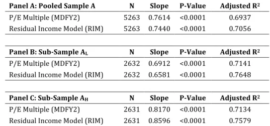
This chapter analyses whether a large gap between a firm’s operational performance and its market price implies that valuation models are less accurate. It has been suggested in literature that a high P/OP makes it more difficult to link a firm’s valuation with its accounting numbers (Trueman et al., 2000). Thus, the aim of this chapter is to find if empirical evidence support the claim that a high Price to Operating Income (P/OI) translates into a worse performance of valuation models.
As a proxy for operational performance, Operating Income Before Depreciation (OIBDP) was selected since it best mirrors the firm’s operational status quo, isolating influences that hide true operational performance. In the numerator of the abovementioned ratio lays the share price in April. The valuation models used for this study are the RIM and the Price-‐Earnings (P/E) multiple.
The following section presents the hypotheses developed and after the research design methodology is described. The final sections include the analysis of results and the concluding remarks.
3.1.2 Hypotheses Development
The hypotheses posited in this dissertation are derived from the rationale presented in chapter 1 and crafted by the insights retrieved from chapter 2:
• H1: High Price to Operating Income implies poorer performance of
valuation models, P/E Multiple and RIM, relative to low P/OI;
• H2: The level of performance is not equal across years; • H3: The level of performance is not equal across industries;
• H4: The P/E multiples-‐based valuation model performs better than the RIM
when applied to high P/OI firms.
The first hypothesis (H1) is based on the difficulty of valuing firms which market price is well above its operating performance (Trueman et al., 2000).
As economic conditions deteriorate, it is posited that the effect of poorer performance of valuation models will be exacerbated. This means that for years of economic crisis the average performance of valuations models is expected to be worse, resulting in performance differences across years (H2).
Similarly, it is expected that industries will be more or less exposed to the high P/OI effect due to industry-‐specific characteristics (H3).
Finally, since H1 implies that accounting numbers are less connected to firm value in high P/OI companies, the RIM is expected to be a worse value predictor since it requires more fundamentals’ input than the P/E, which better reflects the market valuation (H4).
3.2 Research Design
3.2.1 Sample Selection
The initial dataset contained 10,432 observations of U.S. firms with publicly
traded common stocks between 2007-‐20123. Furthermore, these were
nonfinancial firms4 whose fiscal years ended in December. Adding to that, their
share prices were at least $1 and they were followed by at least one analyst. Finally, total assets, revenues, number of shares outstanding, and the adjustment factor were positive.
The sample selection process is presented in table 1. The first criterion applied was that observations missing the median of 1 or 2-‐year-‐ahead earnings per share (EPS) forecasts (mdfy1 and mdfy2, respectively) or missing operating income before depreciation (OIBDP) were deleted. This was due to valuation model requirements and to enable the sample split into high and low P/OI.
The following step was to eliminate observations with less than 3 mdfy2 forecasts for its year and SIC3 code group in order to have a meaningful harmonic mean benchmark multiple at SIC3 level5.
To guarantee that the cost of equity capital is computed with positive beta, 47 observations were withdrawn. Valuation model requirements forced the elimination of observations with non-‐positive EPS, BVE per share (BPS) or mdfy1 or mdfy2.
Then the final exclusion took place due to non-‐positive P/E estimates. Sample trimming followed with cut-‐off defined at 1% in order to eliminate extreme observations that would misrepresent the population.
The last stage consisted in the separation of the final sample (A) into high (AH)
and low (AL) P/OI. It was defined that high P/OI was above the median of the
ratio6.
3 Fiscal years 2006-‐2011.
4 SIC2 code groups were not 60-‐69.
5 Since Alford (1992) showed that at such level performance is increased.
6 Other options were considered such as setting high (low) above the third (below the first) quartile, but
were not employed in order to keep a greater number of observations and consequently higher statistical power.
Additionally, two other samples of high and low P/OI were created: B7 and C8. So
that the median is significant, for C observations with less than six SIC3 group observations were excluded. Three different samples were created to verify if (and how) the analysis varies according to the definition of high/low P/OI.
Table 1 – Sample Selection Process Number of
Observations Observations of U.S. public firms between 2007 and 2012 10432 Observations with missing median of 1 (mdfy1) or 2-‐year (mdfy2)
ahead EPS forecasts or OIBDP (Op. Income Before Depr.) (1897) Observations with less than 3 mdfy2 forecasts for its year and SIC3 code
group (728)
Observations with missing or non-‐positive beta (47) Observations with non-‐positive book value of equity per share (279) Observations with non-‐positive earnings per share (1316) Observations with non-‐positive mdfy1 or mdfy2 (143) Observations with non-‐positive P/E valuations (87) Observations trimmed with cut-‐off set at 1% (672)
Final sample of U.S. public firms between 2007 and 2012 5263
A Sub-‐sample AH: high P/OI firms 2631
Sub-‐sample AL: low P/OI firms 2632
B Sub-‐sample BH: high P/OI firms 2630
Sub-‐sample BL: low P/OI firms 2633
Observations eliminated due to less than 6 firms present in SIC3 group (65) Final sample of U.S. public firms between 2007 and 2012 5198
C Sub-‐sample CH: high P/OI firms 2573
Sub-‐sample CL: low P/OI firms 2625
3.2.2 Data and Variable Definitions
The data for the original sample was retrieved from Compustat9, I/B/E/S10, and
CRSP11. Table 2 lists the variables used in the large sample analysis12:
7 Instead of using the whole sample’s median, highs (lows) were defined as above (equal or below) the
median P/OI of their year (sub-‐sample B).
8 The same process was applied but with the median P/OI of each SIC3 group (sub-‐sample C). 9 Compustat provides information regarding firms’ reported accounting numbers.