Performance Evaluation of a
Web-Service-Based DMCS
Vítor Viegas
1,2, Pedro Girão
2, Miguel Dias Pereira
1,2 1ESTSetúbal-LabIM, Instituto Politécnico de Setúbal, Setúbal, Portugal
2
Instituto de Telecomunicações, Lisboa, Portugal Email: [email protected]
Abstract – The paper describes a set of experiments conducted on
a service-oriented middleware infrastructure in order to evaluate its performance and applicability in the context of Distributed Measurement and Control Systems (DMCS). The infrastructure, entirely based on Web Services, was built using the Windows Communication Foundation (WCF), a software package released by Microsoft to develop distributed applications. The experiments were performed on a real plant equipped with all the instrumentation needed to run control loops for pressure, level, flow and temperature, quantities widely found in the process industry. The work focus on measuring the time delays associated with control loops and remote calls. The methodology of each experiment is described, results are presented and conclusions are drawn.
Keywords – Web Service, DMCS, process, time delay, network traffic
I. INTRODUCTION
The explosion of the Internet in the 1990’s brought new challenges and new opportunities to the software industry. The market claimed for new products in areas such as browsing, multimedia and distributed applications in general. Companies worked day and night to fill market needs and to conquer new clients by proposing innovative solutions. The need to produce more and better code in less time could only be compensated by improving software productivity. This became possible with the release of new development frameworks that include last-generation programming languages, pre-built code libraries, intuitive debugging tools and high-performance virtual machines. Two well-known examples of such frameworks are the Java Platform and the .NET Framework.
The Java Platform [1-2] was released by Sun Microsystems in 1996. It refers to a set of components that together allow the development and execution of applications written in the Java programming language. Java is used in a wide variety of environments from embedded devices and mobile phones to desktop computers and enterprise servers. The platform is composed by three main components:
• Java language: The Java language borrows heavily
from C and C++ but it adds high-level facilities such as
automatic memory management, security and
threading. The high-level code is compiled to an intermediate language known as “Java bytecode”.
• Java Virtual Machine (JVM): The JVM executes Java
bytecode, which is the same no matter what hardware or operating system the program is running under. The JVM takes the Java bytecode and compiles it to native processor instructions by using a just-in-time compiler. Although Java applications are platform independent, the code of the JVM is not; every supported processor and operating system has its own JVM.
• Class libraries: The Java Platform provides a vast set of
dynamically loadable libraries that can be used by the programmer to perform common tasks. Thousands of pre-built classes are available to construct graphical user interfaces, interact with databases, handle network communications, access files and so on.
The success of Java and its concept of write once and run
anywhere has led to other similar efforts, notably the .NET
Framework released by Microsoft in 2002. The .NET Framework [3-4] is targeted for the development and execution of applications in the Windows operating system (although in theory any other operating system can be used as well). The framework is composed by three main components:
• New programming languages: Microsoft released two
new programming languages to serve the purposes of the .NET Framework: the C# which is a kind of modern Java; and VB.NET which is the evolution of Visual Basic. The high-level code is compiled into an intermediate language known as “Microsoft Common Intermediate Language” (MSIL).
• Common Language Runtime (CLR): The CLR is a
virtual machine – conceptually similar to the JVM – that executes MSIL.
• Class libraries: Like the Java Platform, the .NET
Framework also provides a vast set of pre-built classes to simplify the programmer’s job. Correlated classes are grouped in software packages according their functional affinities. A good example is the Windows Communication Foundation (WCF) [5], a package that provides the essential off-the-shelf plumbing required to develop secure, reliable and interoperable distributed applications.
The gains concerning software productivity were followed by the development of cross-platform Web Service-oriented
applications [6-7]. These applications cooperate in
heterogeneous environments like the Internet by calling remote methods (services) between them. Interoperability is achieved by imposing standards that describe the behavior of the service and the way to access it, regardless of its underlying implementation. This idea is not new, but new is the fact that Web Services are getting a wide acceptance among the software community. Because they are supported by all the major software companies around the world (such as IBM, Microsoft and Sun Microsystems), Web Services have the chance to become the first widely used middleware solution and the answer for many interoperability problems.
The advances in terms of software productivity and interoperability are very tempting to be used in the context of Distributed Measurement and Control Systems (DMCS). Following this idea, the authors present a DMCS that takes advantage of the productivity supplied by the .NET Framework and the interoperability provided by Web Services. Nevertheless, this strategy has some pitfalls and drawbacks, in particular those related with the overhead introduced by additional software layers involved in data transfer and processing. This overhead can be evaluated by measuring the time delays associated with control loops and remote calls as proposed in this paper. The results obtained can serve as guidelines and benchmarks for the future.
The paper is organized as follows: section II describes the service-based DMCS prototype used as reference model; section III describes the physical process used as test bench; section IV reports the experiments conducted; and section V extracts conclusions.
II. DMCSPROTOTYPE
The DMCS prototype was presented by the authors in [8]. The system is composed by several computer stations that connect to a Local Area Network (LAN). All computers are equipped with the Windows XP operating system plus .NET Framework 3.5. Two types of stations must be considered:
• Control stations: The control station is an application that executes one or more control loops, alone or in collaboration with other control stations.
• Engineering stations: The engineering station is an
application that performs configuration and monitoring tasks. The configuration process involves the discovery of all stations present in the system and the ability to invoke remote methods on them. The monitoring process implies the interception and logging of all remote variables each time they are updated.
All stations follow the information model proposed by the IEEE 1451.1 Std [9], making them Network Capable Application Processors (NCAP). Each station is an object-oriented application that creates and manipulates
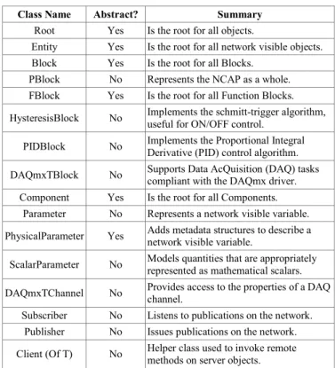
1451.1-Blocks and -Components. These objects were previously coded in VB.NET 2008 and assembled as a reusable Dynamic Link Library (DLL). The library is composed by 16 classes forming a fully functional subset of the 1451.1 object model (see table 1).
TABLE I. SUBSET OF THE 1451.1 OBJECT MODEL
Class Name Abstract? Summary
Root Yes Is the root for all objects.
Entity Yes Is the root for all network visible objects. Block Yes Is the root for all Blocks.
PBlock No Represents the NCAP as a whole. FBlock Yes Is the root for all Function Blocks. HysteresisBlock No Implements the schmitt-trigger algorithm,
useful for ON/OFF control. PIDBlock No Implements the Proportional Integral
Derivative (PID) control algorithm. DAQmxTBlock No Supports Data AcQuisition (DAQ) tasks
compliant with the DAQmx driver. Component Yes Is the root for all Components.
Parameter No Represents a network visible variable. PhysicalParameter Yes Adds metadata structures to describe a network visible variable. ScalarParameter No Models quantities that are appropriately
represented as mathematical scalars. DAQmxTChannel No Provides access to the properties of a DAQ
channel.
Subscriber No Listens to publications on the network. Publisher No Issues publications on the network. Client (Of T) No Helper class used to invoke remote
methods on server objects.
On the field side, control stations work with DAQ boards compliant with the DAQmx driver from National Instruments (NI). Field sensors/actuators are respectively connected to input/output channels of DAQ boards. Each DAQ channel can be automatically configured by reading the Transducer Electronic Data Sheet (TEDS) of the attached transducer according the directives of the 1451.4 Std [10]. Individual field variables are well represented by 1451.1-ScalarParameter objects.
On the network side, inter-station communications are completely based on Web Services. All 1451.1 objects are implemented as WCF Web Services following the best practices described in the literature [11]. Whenever a service is created, it registers itself on a HyperText Transfer Protocol (HTTP) endpoint and exposes its methods on the network. If a client wants to invoke a method, it gets the dispatch address of the service, creates a proxy at run-time, executes the remote call and waits for results (if any). No security credentials are used.
As shown in figure 1, the control station provides a Graphical User Interface (GUI) through which the operator can view and edit the values of loop variables.
III. PHYSICAL PROCESS
The DMCS prototype was customized for the physical process represented in figure 2. The process is a training plant – model TE34 from Plint&Partners Ltd – that includes all the instrumentation needed to run the following control loops:
• Pressure loop: The pressure inside the closed tank C2 is measured by the transmitter PT and is controlled by operating the control valves PCV1 and PCV2 (which form a complementary pair). The pressure increases when PCV1 opens while PCV2 closes, and vice-versa.
• Level loop: The water level inside C2 is measured by
the transmitter LT and is controlled by operating the control valves FCV1 and FCV2 (which also form a complementary pair). The water is continuously pumped from the open tank C1 to the closed tank and returns back through the hand valve HV.
• Temperature loop: The temperature of the water
entering in C1 is measured by the transmitter TT1 and
is controlled by operating the control valve TCV. In alternative, the temperature of the water inside C1 can be considered by using the transmitter TT2. The flow of hot water is constant while the flow of cold water can be adjusted. The open tank is equipped with an overflow tube connected to the drain.
Table 2 lists all the instruments installed on the plant. The connection of the pneumatic instruments to the control stations was done using pressure-to-voltage converters (for the transmitters) and voltage-to-pressure converters (for the control valves). All converters, transmitters and control valves were properly calibrated before experiments took place.
TABLE II. FIELD INSTRUMENTS
Tag Manufacturer Model Signal Summary
PT FOXBORO 821GM-IS1NM1-A 4-20 mA Pressure transmitter PCV1 MASONEILAN 29000 0.2-1 bar Pressure control valve PCV2 MASONEILAN 29000 0.2-1 bar Pressure control valve
LT FOXBORO 15A-LS1-R 0.2-1 bar Level transmitter FCV1 MASONEILAN 29000 0.2-1 bar Flow control valve FCV2 MASONEILAN 29000 0.2-1 bar Flow control valve FT FOXBORO 15A-LS1 0.2-1 bar Orifice flowmeter TT1 FOXBORO E94-P625 4-20 mA Temperature transmitter TT2 FOXBORO E94-P625 4-20 mA Temperature transmitter TCV MASONEILAN 29000 0.2-1 bar Temperature control valve
Two control stations were used to execute the control loops: the pressure and level loops were assigned to control station number one (CS1) and the temperature loop was assigned to control station number two (CS2). Both control stations were equipped with identical DAQ boards – model USB-6008 from NI. Table 3 summarizes the connections between the field instruments and the control stations.
TABLE III. FIELD CONNECTIONS
Station DAQ Channel Connects To
CS1 AI0 (a) PT AI1 LT AI2 FT AO0 (b) PCV1 and PCV2 AO1 FCV1 and FCV2 CS2 AI0 TT1 AI1 TT2 AO0 TCV
(a) Analog Input (b) Analog Output Finally, an engineering station (ES) was added to configure and monitor the control loops. The three stations were installed on three distinct machines, all having the same characteristics as described in table 4. The three computers were connected to an 8 port hub – model 3C16753 from 3Com – forming a private 100 Mbit Ethernet LAN. Figure 3 presents the topology of the final system.
Figure 1. Control station.
TABLE IV. COMPUTATIONAL SUPPORT
Component Description
Motherboard INTEL ESSENTIAL DG41RQ
Processor INTEL PENTIUM DUAL CORE E5300, 2.6 GHz Memory 4 GB of RAM DDR2 800 Mhz
Hard disk SEAGATE 320 GB SATA II ST3320613AS Operating system Windows XP Home SP3 plus .NET Framework 3.5
IV. EXPERIMENTAL RESULTS
A. Cycle Time
Each control station acts like a Programmable Logic Controller (PLC) by running a timed loop on a dedicated thread with priority above normal. On every loop iteration, data is acquired from transmitters, the control routine is executed and actuation values are written to control valves, by this order. Precise timing is achieved by performing passive waits with a resolution of 1 ms. The elapsed time between iterations – called “cycle time” – determines the sampling frequency of the control station and has a strong impact on the quality of control algorithms.
To evaluate the cycle time of the proposed DMCS a set of experiments were done involving the station control CS1 (because it is more loaded than CS2). The following methodology was adopted:
1. A Stopwatch object [12] was added to the timed loop in order to measure the elapsed time between iterations with a resolution of 1/2.6 GHz < 39 ns.
2. The CS1 was started assuming a nominal time cycle of 100 ms. About 1000 samples of effective cycle time were acquired and logged in a file.
3. Step 2 was repeated for the following nominal values: 50 ms, 200 ms and 1000 ms. Figure 4 presents the distribution of the samples for 50 ms and 100 ms. Table 5 summarizes the results of all experiments.
TABLE V. CYCLE TIME OF CS1
Nominal Value (ms)
Effective Value (ms) Mean Relative Error (a) (%)
Centered Samples (b) (%)
Mean Min Max
50 60,19 57 65 20,38 0
100 100,48 100 101 0,480 100
200 200,52 200 201 0,260 100
1000 1000,46 1000 1001 0,046 100
(a) Defined as 100 × |Nominal Value - Mean Effective Value| / Nominal Value. (b) Percentage of samples inside the interval Nominal Value ± 1 ms. The collected data can be analyzed as follows:
• Above 100 ms inclusive, the mean value of effective
cycle time is very close to the nominal value. The mean relative error tends to decrease suggesting that bigger cycle times are more accurate.
• Above 100 ms inclusive, the percentage of centered
samples is 100%, meaning that Windows performs reasonably well although is not a real-time operating system.
• Below 100 ms the nominal cycle time is not satisfied.
The minimum mean value of effective cycle time is approximately 60 ms, which corresponds to a maximum sampling frequency of 16 Hz. Given the inertia of the physical process, a sampling frequency of 5 Hz is sufficient to control it.
B. Communication Delay
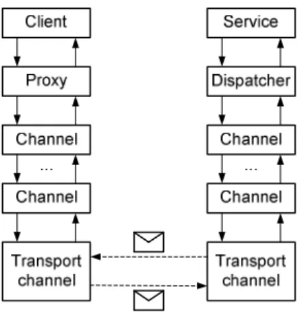
Web Services are natively prepared to implement the client/server communication model. When the client creates a proxy and executes a remote call a lot of work is done behind the scenes (see figure 5):
1. The proxy serializes the call stack frame to a message and sends it down to a chain of channels.
2. A channel is merely an interceptor, whose purpose is to perform a specific task like formatting the message or adding security credentials. The default formatter implements the Simple Object Access Protocol (SOAP) [13], which is targeted for cross-platform
Figure 3. Topology of the final system.
Figure 4. Effective cycle time occurrences (black circles for a nominal value of 50 ms and black squares for a nominal value of 100 ms).
communications. The WCF allows the creation of custom channels to meet special requirements.
3. The last channel on the client side – the transport channel – sends the SOAP message over the configured transport (such as HTTP).
4. On the host side, the message goes through a chain of channels that perform operations such as security checking and message de-formatting. The last channel passes the message to the dispatcher, which converts it to a stack frame and calls the service locally.
5. The service executes the call and returns control to the dispatcher, which then converts the returned values and error information (if any) to a return message.
6. The return message flows in the opposite direction: it passes through the host-side channels, then the client-side channels and arrives to the proxy, which converts it to a stack frame and returns control to the client.
The layered structure depicted in figure 5 is very flexible but introduces a great amount of delay in the communication path between the client and the server. This delay interferes with the sampling frequency of distributed control loops and degrades the responsiveness of the whole system.
To evaluate the communication delay of the proposed DMCS a set of experiments were done adopting the following methodology:
1. The cycle time of all control stations was adjusted to 200 ms. The control routine of CS1 was modified to periodically read the setpoint of the temperature loop running in CS2. In this scenario CS1 is the client and CS2 is the server.
2. Two instructions were added on the client side, immediately before and after the remote call, in order to generate a positive pulse on the data bits of the client’s parallel port. This pulse defines the amount of
time that the read operation takes to execute (including the communication delay).
3. Two instructions were also added on the server side, one at the beginning of the service and the other at the end, in order to generate a positive pulse on the data bits of the server’s parallel port. This pulse defines the amount of time that the read operation takes to be serviced (excluding the communication delay).
4. Both pulsed signals were connected to a XOR gate to discriminate two communication delays (see figure 6):
τ1 representing the client-to-sever delay, and τ2
representing the server-to-client delay.
5. A Virtual Instrument (VI) was built in LabVIEW to
measure τ1 and τ2. The VI runs on a dedicated
computer equipped with a DAQ board – model PCI-6024E from NI – that provides two 24-bit counters. The counter 0 was used to measure pulse width with a resolution of 1/20 MHz = 5 ns.
6. The process was started and all stations were launched. About 1000 samples of τ1 and τ2 were acquired and
processed. Figure 7 presents the corresponding distribution of τ1.
7. The network was loaded by connecting two more computers to the hub. These computers were programmed to exchange large amounts of data between them using Transmission Control Protocol (TCP) sockets. Step 6 was repeated for the following values of traffic load: 6%, 12%, 25%, 50% and 70%. Figure 8 presents the distribution of τ1 for a traffic load
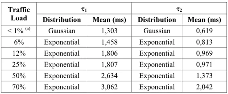
of 50%. Table 6 summarizes the results of all experiments.
The collected data can be analyzed as follows:
• The communication delay (τ1 + τ2) is in the range of
few ms.
• The delay τ1 is longer than the delay τ2 because the
client-to-server message is bigger than the return message.
• For low traffic loads (less than 1% as is the case of
figure 7) the delays τ1 and τ2 have Gaussian
distributions, which are justified by the random behavior of the Windows scheduler.
• For higher traffic loads (as is the case of figure 8) the
delays τ1 and τ2 have exponential distributions, which
are justified by the contention in the network. These distributions are in agreement with the queueing theory [14], which is accepted as a valid mathematical model for Ethernet.
• The delays τ1 and τ2 become longer as the contention
in the network worsens.
V. CONCLUSIONS
An innovative DMCS was presented in this paper. The system takes advantage of the productivity supplied by the .NET Framework and the interoperability provided by Web Services. The performance of the proposed solution was evaluated by measuring the maximum achievable sampling frequency and the communication delay of remote calls.
In terms of sampling frequency, results were obtained for a control station running two control loops. The control station performed well for sampling frequencies of 10 Hz or lower. Given the inertia of the physical process, a sampling frequency of 5 Hz was adopted with good results.
In terms of communication delay, the following conclusions shall be retained:
• The communication delay is in the range of few ms,
becoming longer as the contention in the network worsens.
• The client-to-server and server-to-client delays depend
on the size of the underlying SOAP messages.
• For low traffic loads the communication delay has
Gaussian distribution justified by the random behavior of the Windows scheduler.
• For higher traffic loads the communication delay has
exponential distribution justified by the contention in the network.
REFERENCES [1] http://www.sun.com/java
[2] http://java.sun.com/docs/books/tutorial
[3] David S. Platt, “Introducing Microsoft .NET”, 3rd Edition, Microsoft Press, USA, 2003, ISBN 0-7356-1918-2
[4] http://msdn2.microsoft.com/en-us/netframework/default.aspx
[5] http://msdn2.microsoft.com/en-us/netframework/aa663324.aspx
[6] http://www.w3.org/TR/ws-arch
[7] Adam Freeman, Allen Jones, “Microsoft .NET, XML Web Services Step by Step”, Microsoft Press, USA, 2003, ISBN 0-7356-1720-1
[8] Vítor Viegas, P. Silva Girão, J. M. Dias Pereira, “Open Controller for Distributed Instrumentation Systems”, IEEE International Workshop on Intelligent Data Acquisition and Advanced Computing Systems (IDAACS) – Technology and Applications, Rende, Cosenza, Italy, September 2009
[9] IEEE Std. 1451.1-1999, “IEEE Standard for a Smart Transducer Interface for Sensors and Actuators – Network Capable Application Processor (NCAP) Information Model”
[10] IEEE Std. 1451.4, “IEEE Standard for a Smart Transducer Interface for Sensors and Actuators – Mixed-Mode Communication Protocols and Transducer Electronic Datasheet (TEDS) Formats”, USA, 2004 [11] Juval Lowy, “Programming WCF Services”, O’Reilly, USA, 2007,
ISBN 0-596-52699-7
[12] http://msdn.microsoft.com/en-us/library/system.diagnostics.stopwatch.aspx
[13] http://www.w3schools.com/soap/default.asp
[14] Gerd E. Keiser, “Local Area Networks”, McGraw-Hill, 1989, ISBN 0-07-100380-0
Figure 6. Communication delays τ1 and τ2.
Figure 7. Distribution of τ1 with no extra traffic load.
Figure 8. Distribution of τ1 with traffic load = 50%.
TABLE VI. COMMUNICATION DELAYS FOR VARIOUS VALUES OF TRAFFIC LOAD Traffic Load τ τ τ τ1 ττττ2
Distribution Mean (ms) Distribution Mean (ms)
< 1% (a) Gaussian 1,303 Gaussian 0,619
6% Exponential 1,458 Exponential 0,813 12% Exponential 1,806 Exponential 0,969 25% Exponential 1,807 Exponential 0,971 50% Exponential 2,634 Exponential 1,373 70% Exponential 3,062 Exponential 2,042