Velocity control of a two DOF walking system

Outubro de 2012

Universidade do Minho

Escola de Engenharia

José Pedro do Carmo Pontes

Velocity Control of a Two DOF Walking

System

Dissertação de Mestrado

Mestrado Integrado em Engenharia Biomédica

Trabalho realizado sob a orientação da

Professora Doutora Cristina Manuela Peixoto

dos Santos

Outubro de 2012

José Pedro do Carmo Pontes

Velocity Control of a Two DOF Walking

System

É AUTORIZADA A REPRODUÇÃO INTEGRAL DESTA DISSERTAÇÃO APENAS PARA EFEITOS DE INVESTIGAÇÃO, MEDIANTE DECLARAÇÃO ESCRITA DO INTERESSADO, QUE A TAL SE

COMPROMETE;

Universidade do Minho, ___/___/______

I gratefully acknowledge the opportunity made by the Professor Cristina Manuela Peixoto Santos to integrate the ABSG group, and for introducing me to several very interesting subjects. I am grateful for the opportunity to learn as much as I could. I would like to thank all the help she gave me through the execution of my work, from the insightful discussions to the uncountable advice.

Lastly, I would like to acknowledge the good environment in the lab and the pleasant time spent with all my colleagues. Specially MSc. Vítor Santos for all the help he was patiently able to provide.

This work is funded by FEDER Funding supported by the Operational Program Competi-tive Factors - COMPETE and National Funding supported by the FCT - Portuguese Science Foundation through project PTDC/EEACRO/100655/2008. Pedro Pontes is supported by grant UMINHO/BI/78/2012.

Resumo

O controlo baseado em Central Pattern Generators (CPG) de sistemas locomoção per-mite um tipo de modulação que é direta e condicionada ao controlo dos parâmetros da rede. A implementação de tal controlo requer o conhecimento do mapeamento entre estes parâmetros e as variáveis que definem a locomoção. Uma abordagem a este problema consiste em usar métodos de Machine Learning. Neste trabalho, usando regressão linear múltipla, e, num estado mais tardio, Locally Weighted Projection Regression (LWPR), tentei manter a velocidade média de um sistema de locomoção de dois graus de liberdade. LWPR mostrou boas indicações de ser capaz de uma forma robusta e fácil de implementar de controlar certos aspectos da locomoção, havendo no entanto muito espaço para melhorar.

The Central Pattern Generator (CPG) based control of locomotor systems allows for a type of modulation that is straightforward and constrained to the control of the network parameters. The implementation of such control requires the knowledge of the mapping between this parameters and the variables that define the locomotion. One approach to this problem consists in calling upon machine learning methods. In this work, using Multiple Linear Regression, and, in a later stage, Locally Weighted Projection Regression (LWPR), we try to maintain the average velocity of a two Degree Of Freedom walking system. LWPR showed good indications of being able to provide an easy to implement and robust way of controlling certain aspects of the locomotion, with there still being much room for improvement.

Contents

2 State of the Art 7 2.1 Learning control . . . 7

2.2 Model based learning . . . 8

2.3 Model-free learning . . . 9

2.4 Reinforcement learning . . . 10

2.5 Learning in CPG based control . . . 11

2.6 Locally Weighted Learning . . . 13

3 Bio-Inspired Architecture 15 3.1 Neural structures for locomotion in vertebrates . . . 15

3.2 Central Pattern Generators . . . 17 vi

4 Velocity control of a two DOF walking system 19

4.1 System description . . . 19

4.2 Locomotion controller design . . . 20

4.2.1 Step phases frequency modulation . . . 24

4.2.2 The CPG network . . . 24

4.3 Problem formulation . . . 26

4.3.1 Control using a forward model . . . 27

4.3.2 Control using an inverse model . . . 28

5 Velocity control using a forward model 31 5.1 Velocity characterization conditions . . . 31

5.2 Velocity characterization . . . 32

5.2.1 Multiple linear regression approximation . . . 34

5.3 Maintaining the mean velocity . . . 35

5.4 Results . . . 38

6 Velocity control using an inverse model 39 6.1 Training in the simulated environment . . . 40

6.2 Obtaining the LWPR model . . . 43

6.3 Results for the control with the first model . . . 46

6.4 Velocity control while transversing a ramp . . . 47

7 Conclusions 61 7.1 Future work . . . 62

List of Figures

3.1 Basic concept of the central nervous system and the peripheral nervous system on a vertebrate [1]. . . 16 3.2 Basic concept of the central nervous system and the peripheral nervous

system on a vertebrate [1]. . . 17

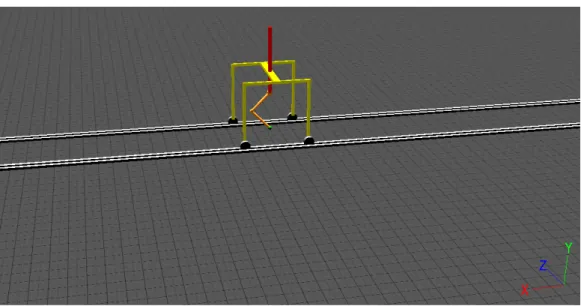
4.1 Simulated environment for the second stage testing. . . 20 4.2 Solutions for the oscillator when (a), (c) µ =−1 and (b), (d) µ = 1.

Initial condition (x₀, y₀) = (0.5,−0.5), O = 0, α =β = 1, ω = 6.3rad.s−1. In (c) and (d) the x state variable is the solid blue line and the y state variable is the dashed green line. . . . 21 4.3 Two different solutions for the oscillator withµ= 1, O = 0,ω= 6.3rad.s−1

for both solutions. The solid red line represents a solution with_β = 10 andα= 0.1 and the dashed blue line represents a solution withβ = 0.1 and_α= 10. . . 22 viii

4.4 State variables of the Hopf oscillator, in function of time, for a specific so-lution withµ= 1, O = 0, andα=β= 1. The solid blue line represents

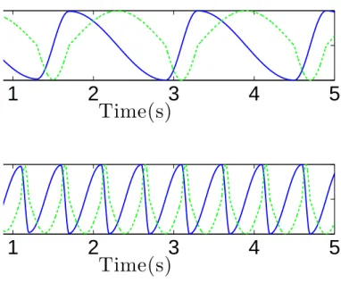
x and the dashed green line y. The parameterω starts at 6.3rad.s−1, is changed to_−6.3rad.s−1 at t = 2s and to_−1.57rad.s−1at t = 6s. 23 4.5 Solutions for the oscillator withβ = 0.75 (top) andβ= 0.2 (bottom), for

a_ωswing≈ 7.85rad.s−1(Tsw = 0.4s). The solid blue line represents x and the dashed green line represents y. The duration of the swing phase --- negative phase of y (the ascending phase of x) is kept constant --- and only the the stance phase duration changes. . . 25 5.1 Simulated world on WEBOTS, for the first, second, and third experiments

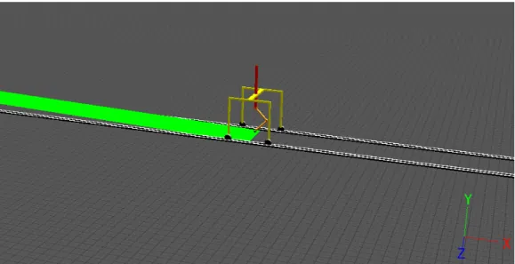
of the first stage. . . 33 5.2 Simulated world on WEBOTS, for the fifth, sixth and seventh experiments

of the first stage. . . 33 5.3 Simulated world on WEBOTS, for the seventh, eight and ninth experiments

of the first stage. . . 34 5.4 Speed characterization of the robot for different values of_ωand Tswing=

0.9. The plots correspond to the experiments numbered from 1 to 9, in the order from left to right, and from top to bottom. The experiment observations are plotted in a dotted line, while the regression model is plotted in a solid line. The values of the r2 _{statistic for each regression}

are also shown. . . 36 5.5 Simulated world on WEBOTS, for the second stage. . . 37 5.6 Mean velocity against time, for the second stage. . . 38

List of Figures x

6.1 Simulated environment used in the first training and first and second sets of tests for this stage of the work. . . 41 6.2 Simulated environment used in the second training for this stage of the

work. . . 41 6.3 Simulated environment used in the third set of tests for this stage of the

work. . . 42 6.4 Data from the first training phase used in the regression. . . 44 6.5 Example regression test set results for the first training phase. The test

data points are the desired output (vavgin m.s−1), with the corresponding control point (T, inseconds). The solid red line shows the data collected during training, and the blue dashed line shows a) the predictions and the b) confidence bounds. . . 45 6.6 Output (vavg) and control (Tswing) variables against time, for the first

con-trol test, desired vavg of 0.06 m.s−1, all three trials. . . 48 6.7 Output (vavg) and control (Tswing) variables against time, for the first

con-trol test, desired vavg of 0.09 m.s−1, all three trials. . . 49 6.8 Output (v_avg) and control (T_swing) variables against time, for the first

con-trol test, desired vavg of 0.12 m.s−1, all three trials. . . 50 6.9 Output (vavg) and control (Tswing) variables against time, for the second

control test, desired vavg of 0.06 m.s−1, all three trials. The solid blue lines show the values for vavg and Tswing. The vertical dashed red lines show the points in time where a change of mass occurred, while the horizontal show the desired velocity for the test. . . 51

6.10 Output (vavg) and control (Tswing) variables against time, for the second control test, desired vavg of 0.09 m.s−1, all three trials. The solid blue lines show the values for vavg and Tswing. The vertical dashed red lines show the points in time where a change of mass occurred, while the horizontal show the desired velocity for the test. . . 52 6.11 Output (vavg) and control (Tswing) variables against time, for the second

control test, desired v_avg of 0.12 m.s−1, all three trials. The solid blue lines show the values for vavg and Tswing. The vertical dashed red lines show the points in time where a change of mass occurred, while the horizontal show the desired velocity for the test. . . 53 6.12 Data from the second training phase used in the regression. . . 56 6.13 Example regression test set results for the second training phase. The test

data points are the desired output (vavgin m.s−1), with the corresponding control point (T, inseconds). The solid red line shows the data collected during training, and the blue dashed line shows a) the predictions and the b) confidence bounds. . . 57 6.14 Output (vavg) and control (Tswing) variables against time, for the third

control test, desired v_avg of 0.06 m.s−1, all three trials. The solid blue lines show the values for vavgand Tswing. The horizontal dashed red line show the desired velocity for the test. . . 58 6.15 Output (vavg) and control (Tswing) variables against time, for the third

control test, desired vavg of 0.09 m.s−1, all three trials. The solid blue lines show the values for vavgand Tswing. The horizontal dashed red line show the desired velocity for the test. . . 59

List of Figures xii

6.16 Output (vavg) and control (Tswing) variables against time, for the third control test, desired vavg of 0.12 m.s−1, all three trials. The solid blue lines show the values for vavgand Tswing. The horizontal dashed red line show the desired velocity for the test. . . 60

6.1 Results for the first set of test runs. . . 46 6.2 Results for the second set of test runs. . . 54 6.3 Results for the third set of test runs. . . 56

Chapter 1

Introduction

This manuscript presents the work I have been conducting for the past year, while part of the Adaptive System Behaviour Group at Universidade do Minho in Portugal. I took part in the group's research project, with biologically inspired robotic locomotion as a theme and dynamical systems as a tool.

The ultimate goal of the developed research is to improve and develop new controllers for articulated robots, create novel ways of achieving adaptive behaviors and general know how in the field of adaptive dynamic controllers.

1.1

Motivation

Humanoid robotics is often envisioned as one of the potential solutions to the service robotics problem and this field of research is exponentially growing. Scientific contribu-tions in this domain go from intrinsically safe actuator design [40] to high-level social and cognitive interactions [6]. At the control level, several trends have been followed with various level of success.

The requirements for an autonomous robot to coexist with people and to be in highly dy-namic and unpredictable environments are far too great and very demanding. Coordinating many degrees of freedom (DOF) in order to execute certain tasks is also a problem without a general solution. As such, developing solutions for achieving these requirements are still an important focus of study and research.

On uneven and rough terrains that may be comprised of several obstacles walking robots have clear advantage over conventional robots that use wheels or tracks. A walking robot contacts the ground in determined points, allowing the avoidance of obstacles. Further-more, a walking robot can also be omnidirectional.

Despite walking robots providing such advantages when locomotion adaptation is the key, these robotic platforms are also hard to control. The controller of such a robot has to deal with a highly nonlinear system with many degrees of freedom, changes on body dynam-ics and unpredictable dynamdynam-ics related to the robot-environment interaction. The robot must show adequate movements in order to support itself and propel itself through the environment, while not falling over.

3 1.1. Motivation

There is great variety of approaches to design a controller for a walking robot. Some use pre-recorded trajectories to generate templates, others use stability criteria to do online trajectory modulation (locomotion control) [43]. The common point between most of them is the requirement of a perfect knowledge of the robot and environment dynamics. The use of Central Pattern Generators (CPG) to implement control systems for real-time robot walking is a biologically inspired approach that has been growing in popularity in the past years. Robotic platforms have been based on animal structures for many years. Ani-mals present innate abilities to adapt locomotor movements to changes in the environment, exhibit many corrective reflexes and are exceptional explorers of unstructured terrains. These CPG models have been used to control many different type of robots with distinct types of locomotion [16]. Locomotor controllers have been implemented using several type of CPG models. Out of all these models, a system of coupled oscillators shows some interesting properties. The system has the ability to return to its rhythmic behavior after transient perturbations, and is also well suited for distributed implementation along the system to be controlled. By coupling the oscillators and the mechanical system, the natural dynamics of the combined system can be exploited in order to achieve locomotion [44]. These aforementioned type of CPG usually have few control parameters, which allow straight-forward modulation of the locomotion. While the general end result achieved with the tuning of a parameter is usually easy to predict (e.g. lowering the parameter that controls the pe-riod of one stride should increase the locomotion speed), the exact relationship between these parameters and the locomotion they generate depends on the control architecture, the controlled system, external and internal perturbations, and the traversed environment, building up to a big number of variables to take into account, and making an analytical

anal-ysis both very hard and very costly to perform. Learning from experience is the a logical step over this difficulty, because it can provide an easier and more straightforward solution to the problem. Ideally, we want to obtain a mapping of the CPG parameters space and the locomotion predefined criteria. Changing the speed, direction, gait type and clearance, are just some of the possible final goals of the modulation.

1.2

Objectives

This work is a multidisciplinary undertaking that combines principles of dynamical systems theory, neuroscience and robotics. It will enable further contributions to the achievement of goal directed locomotion on an autonomous walking robot. Specifically, it will enable automatic adaptation to environmental changes for a locomotion system through the control of a small set of parameters.

The ultimate goal is to propose a learning control architecture, with a particular focus on adaptive goal-directed locomotion and, more specifically, in speed control.

In order to pursue this main goal it is necessary to achieve the following objectives.

1.

To design, a mathematical model for a Central Pattern Generator, taking in consideration features of its biological counterpart. The model will use nonlinear oscillators, which allow a fast response to stimuli. This makes it well suited for fast adaptive behavior because it

5 1.2. Objectives

turns a high dimensional problem into simple selection of a small number of parameters that control the CPG network.

This model must enable modulation of the generated trajectories, possibly such that it reflects the environment changes. Nonlinear oscillators generate smooth trajectories mod-ulated by simple parameters change [11].

The CPG network is intended to control a simulated walking system consisting in three seg-ments and two rotational joints, suspended in a sliding support.

2.

In a first learning stage the goal is to obtain a relationship between some of the CPG system parameters and the mechanical system average speed throughout a set period of time. This allows for a first approach to velocity control of the designated system, and for a better understanding of the dynamics involved.

3.

On a second learning stage, the aim is to obtain a control structure that allows online learning, adaptation to condition changes, and a short training time, and apply it to the simulated locomotion system. The system is then to be tested in different sets of internal and external conditions, and afterward used that knowledge to maintain the average speed in a test run where those conditions were constantly changed. We apply a state of the art learning algorithm called Locally Weighted Projection Regression (LWPR) [42], that allows online learning, adaptation to condition changes, and a considerable decrease in training

time, which makes it a very desirable approach in order to achieve our objective.

1.3

Outline

This manuscript is organized as follows: Chapter 2 presents an non in-depth view of the nervous systems of vertebrate animals and its circuits involved on locomotion. Chapter 3 contains a brief review of the most revelant work done on the topics discussed on the next chapters. Chapter 4 describes the locomotion system simulated on the experimental part of this work, along with its controller and a more detailed explanation of the tackled control challenges. Chapters 5 and 6 expose the two different approaches used to ultimately attain the initial objectives, Multiple Linear Regression and Locally Weighted Regression, as well as the results obtained with each one. The last Chapter (7) summarizes and presents a discussion of the results, in addition to suggestion for future work.

1.4

Publications

The work carried throughout my participation in the group has led to an accepted submis-sion as a conference participation.

José Pedro Pontes and Cristina P. Santos (2012), "Velocity Control of a Two DOF Walking System" Accepted for Numerical Analysis and Applied Mathematics ICNAAM 2012, AIP Conf. Proc. 1389; 19-25 September 2012, Kypriotis Hotels and Conference Center, Kos, Greece.

Chapter 2

State of the Art

For context and justification of the work exposed in this manuscript, this chapter will ad-dress, to some extent, the state of the art on Machine Learning applied to Robotics. The focus will be on methods applied to locomotion controllers based on nonlinear dynamical systems.

We will evaluate the advantages an disadvantages of the methods used in some of the most important papers in this area, taking into account the specific requirements of the objectives we wanted to achieve.

2.1

Learning control

Machine learning methods were introduced in automatic systems about four decades ago [39]. In the early 1980s there was an emergence of learning control with applications to dynamical systems, such as the development of learning control laws for mechanical systems and the discussion of their applicability on robot manipulators [2, 3]. Learning control refers to the process of acquiring a control strategy for a particular control system and a particular task.

The goal of learning control can generally be formalized in terms of finding a task-specific control policy [9]:

u = f (s,t,α), (2.1)

that maps the continuous state vector x of a control system and its environment, possibly in a time t dependent way, to a continuous control vector u. The parameter vector_α de-notes the problem-specific adjustable parameters in the policyπ. As an example, given the current state of a robot we control, and the environment it traverses, we want to deter-mine which control input (e.g. torque commands for joint actuators) we need to achieve a desirable outcome (e.g. a certain speed or path).

9 2.2. Model based learning

2.2

Model based learning

One simple approach is to learning control is to use methods of function approximation to estimate a forward model f () that uses states and actions to predict outcomes (z) [4]:

z = ˆf (s,t, u), (2.2)

where ˆf() is an approximation of f (). Then a controller is computed based on the esti-mated model, which is a technique belonging to the category of model based learning. Kawamura and Fukao [20] developed a method that interpolates input torque patterns ob-tained through Learning Control in order to create a desired motion with a different speed pattern or time-scale. Learning Control optimizes input patterns at each iteration by velocity or acceleration error (the different between a desired motion and the actual motion). Apply-ing the algorithm in an actual robot can be time and memory space consumApply-ing, if we need many specified motion patterns. Interpolating ideal feedforward input patterns, generating another desired motion, helps in overcoming this difficulty. The authors demonstrated that they could form an arbitrary speed pattern from four motion patterns with different time-scales, if all the spatial trajectories were the same. This approach lacks automatic, online, adaptation to changes in the desired trajectory, not to mention the fact that it constrains the spatial trajectory used.

Model based learning results in indirect control, because it usually requires the computation of the controller after we estimate the model. If instead we aim to learn the policy directly, without detour through model identification, we will be using direct control, with model-free

learning.

2.3

Model-free learning

Model-free methods don't use any explicit information about the dynamics of the robot, the environment, and the interactions between both. This makes them, at a first glance, more appropriate for a task that demands adaptability of the control policy to changes in these systems.

Dynamical movement primitives are non-linear differential equations with attractor dynam-ics [17]. Their output serves as desired trajectories for a robot, which can be learned rapidly, and easily re-scaled in terms of the patterns' amplitude, frequency, and offset. They can be used, as an example, to constitute a dynamic systems model which repre-sents a library of different movements [34]. Being non-linear differential equations, these primitives can also be used as a CPG of a robot. Nakanishi and colleagues [27] developed a framework for learning biped locomotion based on this idea, having demonstrated trajec-tories learned through movement primitives by locally weighted regression. This method provides flexibility in encoding complex movements and the potential capability of improv-ing learned movements through reinforcement learnimprov-ing, with the downside of requirimprov-ing the demonstration of the learned trajectories.

Gams and others [11] produced another work that fits the view that biological movements are constructed of motor primitives: a dynamical system that learns and encodes a peri-odic signal. The system has two layers, one that uses nonlinear oscillators to extract the

11 2.4. Reinforcement learning

fundamental frequency of the input signal, and a second that uses nonparametric regres-sion techniques to learn the waveform, by shaping the attractor landscapes according to demonstrated trajectories. The system requires no prior knowledge of the frequency and waveform of the input, and is able to modulate the learned trajectory in response to external events. The adaptation for a signal with six frequency components achieved identical input and output signals. The system can be expanded to several dimensions, working in parallel for various Degrees of Freedom (DOF) of the signal. The authors tested this approach with a humanoid HOPA-2 robot, using 8 DOF to control de arms. They began by using the system to learn and reproduce simple 2D trajectories made by the end effector, and then tested for more complex trajectories. The system successfully learned both patterns, with frequency adaptation taking longer on the complex patterns due to multiple frequency components.

2.4

Reinforcement learning

Reinforcement learning (RL) studies how systems can learn to optimize their behavior in order to obtain rewards and avoid punishments. As an example, an RL based controller for a biped robot is analogous to a baby's acquisition of biped locomotion along its growth [25]. Large applications of this type of learning require the use of function approximators. Historically, the first approach for this approximation has been estimating a value function, with the action-selection policy represented implicitly as the policy that selects in each state the action with highest estimated value [37, 38] - this is model-based control. In robot control, the computation of the value function or its approximation is difficult, analytically or numerically, because of the enormous size of the state and action spaces. Policy gradient reinforcement learning methods avoid this issue by approximating a policy directly using a

function approximator independent of the value function - a model-free solution. The policy is updated according to the gradient of expected reward with respect to policy parameters [37].

Endo and colleagues [10] developed a learning framework for a CPG-based biped locomo-tion controller using the aforemenlocomo-tioned method. They acquired an appropriate feedback controller within a few thousand trials and the controller obtained in numerical simulation achieved stable walking with a physical 3D hardware full-body humanoid in the real world. Mori and others [25] used a CPG-actor-critic model - a policy gradient method incorporating a value function - which approximates a lower-dimensional projection of a value function, instead of a true value function, which is often an easier and lighter approach. In this method, the actor is a controller that transforms an observation into a control signal, and the critic approximates the value function to predict the gradient of the average cost toward the future. The actor's parameter is updated so that the cost predicted by the critic be-comes small. The RL method was applied to autonomous acquisition of biped locomotion by a biped robot simulator. Computer simulations showed the method was able to train a CPG controller such that the learning process was stable. In order to escape local optima, the actor parameter was re-trained by reinitializing the critic's parameter, which resulted in a lot of training episodes. This makes it difficult to apply the method directly to real robots. One possible solution to such problem is to use an approach that does not require stoping or reseting. Sproewitz and colleagues [36] presented an approach that also uses CPG, but with a gradient-free optimization algorithm - Powell's method. The method achieves online learning by running the optimization algorithm in parallel with the CPG model, with speed of locomotion being the criterion to be optimized. Powell's method is fast, but presents more risk of converging to a local optimum than stochastic methods (such as genetic

al-13 2.5. Learning in CPG based control

gorithms, particle swarm optimization or simulated annealing). Speed result obtained with two gaits from experiments with a quadruped robot showed that the speed can be adjusted monotonically with the frequency and, interestingly, the relation is almost linear in the given frequency range.

Matsubara and others [23] combined a model-based Center of Mass (COM) controller and a model-free RL method to acquire dynamic whole-body movements in humanoid robots. A purely model-based controller considers highly approximated dynamics, which can cause poor tracking performance, and it is affected by modeling errors. While the model-based controller can cope with high-dimensionality, the RL method can improve its performance. The COM controller derives joint angular velocities from the desired COM velocity, while RL is used to acquire a controller that derives the desired COM velocity based on the current state. The authors set the goal of strengthening ball-punching on a Hoap-2 humanoid robot in numerical simulation, through a learning process that focused on a COM movement. The locally optimal punching motion with maximal reward was acquired around 2000 episodes of learning and the acquired cooperative whole-body movement, was shown to be effective even in a real environment.

2.5

Learning in CPG based control

Modeling with nonlinear dynamics systems is mathematically quite difficult; optimization approaches are often much easier to handle with well-established algorithms and software tools [34]. This approaches also have the advantage of giving the opportunity to provide a more general, and more compact, representation of a desired trajectory [18]. Trajectory

modulation allows for the on-line adaptation to changes in goals and the system's environ-ment [11].

Manually tuning the open parameters of a CPG network, in order to achieve a desired be-havior, is a cumbersome, lengthly and inexact process [27]. The speed of locomotion, for example, cannot be expressed as an analytical function of the robot parameters because it depends on the dynamics between the robot and the environment [36]. An optimization algorithm can run in parallel with a CPG network and update its parameters. With dif-ferential equations of second order, even abrupt parameter changes will result in smooth convergence towards a new limit cycle, after a short transition period, which means the robot doesn't need to be stopped between iterations [11, 36].

Evolutionary methods are often used of find the parameters of CPG networks. Saif [32] applied the standard Genetic Algorithm (GA) and the Empire Establishment Algorithm (EEA) -a p-ar-allel GA - to -approxim-ate such p-ar-ameters, but found th-at with th-at -appro-ach le-arning to walk was very time-consuming. He then made and adaptive oscillator that can rapidly learn arbitrary periodic signals in a supervised learning framework, and is completely em-bedded in a dynamical system. He used a 3D simulation of a NAO biped robot, training the adaptive oscillator with sample trajectories provided by a player of a ROBOCUP competition. The NAO robot showed a stable and fast walking pattern after 1.5 hours of adaptation. Sato, Watanabe and Igarashi [33] proposed a combination of GA and Reinforcement Learn-ing for determinLearn-ing parameters of a CPG network, and applied it to a quadruped robot. The CPG inner coefficients are learned by a GA, and the feedback controller and the connection controller are learned by Reinforcement Learning. Additional learning after acquiring a walk-ing behavior is done only by RL, with the inner parameters definwalk-ing a basic walkwalk-ing rhythm.

15 2.6. Locally Weighted Learning

They confirmed that the robot could adapt to new environments by only learning sensory feedbacks and connections among oscillators. Christensen, Larsen and Stoy [8] adopted applied a stochastic optimization learning algorithm to optimize eight open parameters of a CPG network used to control a gait. They used the model-less Simultaneous Perturbation Stochastic Approximation method, which requires only two robot trials with different con-trollers per iteration, independently. They applied the algorithm in an online gait learning experiment on a quadruped robot. The robot, while learning, improved its initial velocity from 0 cm.s−1 to 13 cm.s−1 after eight minutes, and with the final gait learned, without online learning, it moved at 17.5 cm.s−1, which is faster than a manually designed gait. The strategy was successfully applied in two systems with different degrees of freedom and modularity.

2.6

Locally Weighted Learning

Locally weighted learning uses locally weighted training to average, interpolate between, or extrapolate from training data. The most sophisticated approaches to this type of learning typically present a learning structure that allows a multitude of models to join together to make a global approximation, by assigning to each one a certain weight. Each local model is trained independently such that its total number does not affect how complex a function can be learned - complexity is only controlled by the level of adaptability of each model [5]. RFWR is a learning algorithm based on locally weighted learning that uses nonlinear function approximation with structure adaptation, represented by piecewise linear models. Nakan-ishi, Ferreal and Schaal [26] compared four learning schemes for a simple function

approx-imation: Locally Weighted Regression (LWR), LWR with normalized weights, Radial Basis Functions (RBF), and RBF with normalized weights. They found that the RBF networks need more re-organization of previously learned parameters when they increased the number of the local models for the approximation, and that they strong cooperation may cause neg-ative interference on the approximator domain. In addition, both RBF approaches started overfitting at a certain number of local models, while the LWR methods approximation im-proved.

An automatic structure adaptation of the function approximator is useful when the com-plexity and structure of the the function to be approximated are not know beforehand [26].

Chapter 3

Bio-Inspired Architecture

It is clear that animals surpass current robots on walking and moving around in our natural world. On their movements they exhibit many corrective reflexes when faced with unex-pected perturbations, and present an exceptional adaptability in rough terrain.

Throughout many years of evolution the locomotor circuits in the nervous system were extended and improved. These circuits rise in complexity from the small fish to the walking mammal, but share similarities in organization and function which were conserved through evolution.

We take inspiration from nervous systems in hope that these potential mechanism of animal motor control can help on improving the design of adaptive algorithms and controllers, while never abandoning an engineering perspective.

3.1

Neural structures for locomotion in vertebrates

The nervous system is a network of specialized cells that control all bodily functions. It is responsible for sending, receiving and processing nerve impulses throughout the body, controlling all the organs and muscles. As can be seen in Figure 3.1, the nervous system in vertebrate animals is divided in two main parts: the peripheral nervous system (PNS) and the central nervous system (CNS) [19].

The PNS consists in nerve cords constituted by afferent fibers that relay sensory information from the limbs and organs to the CNS, and by efferent fibers which transmit information from the CNS to organs and limbs [14].

The spinal cord receives and processes peripheral sensory information from the skin, mus-cles and limbs, and relays it to the brain. It is divided, from head to trunk, into cervical, thoracic, lumbar and sacral regions. It contains neural circuits that endogenously generate rhythmic patterns. There are several of these circuits in the spinal cord, controlling the rhythmic activity for breathing, swallowing, chewing and walking [19, 14].

3.2

Central Pattern Generators

Central Pattern Generators (CPGs) are found in all vertebrate animals, including humans.They are intrinsic spinal networks composed by rhythmogenic units that carry the endogenously generated limb muscle activation during locomotion [12, 22, 21]. The CPGs are activated through tonic signals from supraspinal regions (Figure 3.2).

19 3.2. Central Pattern Generators

Figure 3.1: Basic concept of the central nervous system and the peripheral nervous system on a vertebrate [1].

Figure 3.2: Basic concept of the central nervous system and the peripheral nervous system on a vertebrate [1].

These circuits were extensively studied: in fish, as the lamprey; in amphibians, like tadpoles, frogs, toads and newts; in reptiles and birds; and in mammals, as cats and dogs [12]. Several experiments in animals show that after transection of the spinal cord and after affer-ent input is abolished, rhythmic locomotor movemaffer-ents are exhibited when applying certain excitatory signals. Also, it was evidenced the generation of fictive locomotion in several spinal preparations. These studies, along many other experiments have provided detailed information about the CPGs and the effects of the sensory information on its generated patterns.

It has been proposed that the CPG for each limb is composed by smaller rhythmogenic cir-cuits, the unit-CPG, each controlling one muscle group of extensors and flexors of a limb, i.e. one unit-CPG controlling one joint in a limb [13]. The organization of the CPG is very

21 3.2. Central Pattern Generators

important when considering the required flexibility when generating the different varieties of limb movements during goal directed locomotion [14]. This intralimb coordination of the generated pattern depends of the limb movements to perform - when walking in differ-ent directions the unit-CPGs must be coordinated in differdiffer-ent ways in order to generate a different activation pattern.

The CPG provides the basic rhythm output for locomotion while integrating powerful com-mands from various sources that serve to initiate or modulate it, meeting the requirements of the environment. They show adaptation to different gait patterns and different walking contexts. Signals from supraspinal, spinal and peripheral structures are continuously in-tegrated by the CPG for the proper expression and short-term adaptation of locomotion, providing a great versatility and flexibility on the performed movements [31, 28].

Chapter 4

Velocity control of a two DOF walking

system

4.1

System description

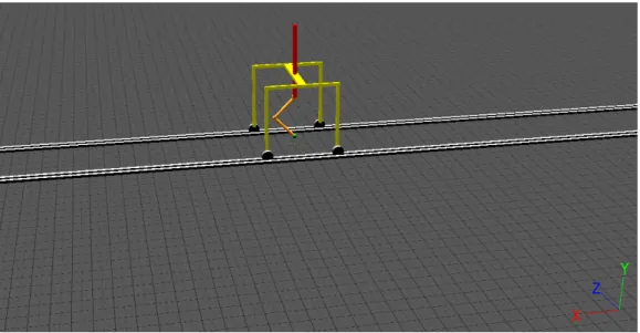
The system used for the simulation (figure 5.1) is comprised by a structure with the very basic structure of a leg intended for hopping, and a supporting sliding platform. The "leg", given this setup, produces a motion similar to a hopping motion, and shall be from now on referred to as the hopper. The hopper has three segments and two actuated joints. The two lower segments are akin to the thigh and foot of a vertebrate's leg, with the joints being comparable to the hip and the ankle. The upper segment keeps the hopper connected to the sliding platform.

With movement from the hopper, the sliding platform will move forward or backwards along the tracks that supports it. This helps the hopper's balance, as well as restraining the movement along a fixed axis.

The work was implemented on this system because of the facility to implement in it a central pattern generator inspired control, and because of the stability it normally offers. As the goal is to analyze the ability to finely tune the parameters of the network to achieve a desired speed, we considered aspects such as the robot's stability and direction control to be secondary, as well as, at least initially, the complexity of the system. The reasoning being that the applied algorithm should be easily expanded to higher dimensions, and capable of processing the extra quantity of information.

The system was simulated on a robot simulation environment called WEBOTS [24], which was developed as a research tool for investigating various control algorithms in mobile robotics.

4.2

Locomotion controller design

The CPG was implemented through the use of a nonlinear dynamical oscillator that presents a Hopf bifurcation [30]. The oscillator is presented as follows,

˙

25 4.2. Locomotion controller design

Figure 4.1: Simulated environment for the second stage testing.

˙

y =α(µ− r2)y +ω(x− O) (4.2)

where x and y are the state variables that present oscillatory harmonic solutions or a stable fixed point, and r = √(x− O)2_{+ y}2_{. The variable} ω _{represents the frequency of the}

oscillator, √_µ represents the amplitude of the oscillations, and_α is a positive constant that controls the speed of convergence to the limit cycle. The variable O is used to control the offset for the solution in the x state variable.

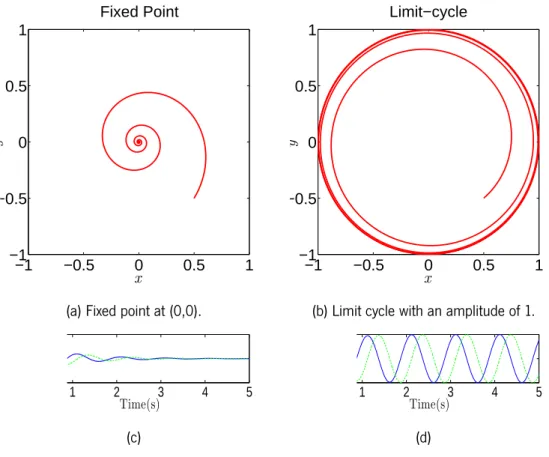
This oscillator relaxes to x = O,y = 0 for values of_µ < 0, and follows a stable orbit when

µ > 0 (Figure 4.2).

Using different speeds of convergence for x and y allows to have a faster convergence on the

−1 −0.5 0 0.5 1 −1 −0.5 0 0.5 1 Fixed Point x y

(a) Fixed point at (0,0).

−1 −0.5 0 0.5 1 −1 −0.5 0 0.5 1 Limit−cycle x y

(b) Limit cycle with an amplitude of 1.

1 2 3 4 5 Time(s) (c) 1 2 3 4 5 Time(s) (d)

Figure 4.2: Solutions for the oscillator when (a), (c) µ =−1 and (b), (d) µ = 1. Initial condition (x₀, y0) = (0.5,−0.5), O = 0,α =β = 1, ω = 6.3rad.s−1. In (c) and (d)

27 4.2. Locomotion controller design

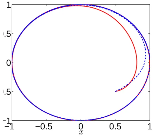
can see that the oscillator solution with the larger value for the parameterβ, which controls the speed of convergence of the y state variable, shows a faster convergence towards the

y axis.

The parameterω specifies the frequency of the oscillations in rad.s−1. The period of the oscillations, or duration of a cycle, T is given by T = 2π

ω, in seconds. Changing the signal

of ω changes the direction of the limit-cycle: for ω > 0 the limit-cycle rotates

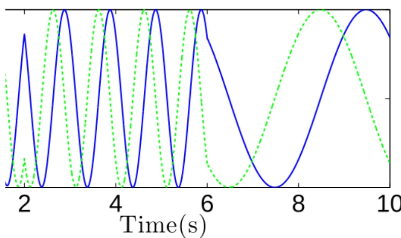
counter-clockwise, and forω< 0 it rotates clock-wise. In Figure 4.4 we can see the effect of both

changing the signal and the module ofω. Notice that when the parameter is altered the oscillator promptly changes the frequency of the generated solution, resulting in a smooth response. We can also verify that with the change in the direction the state variable that was previously trailing behind in time will get ahead (y was trailing behind initially, and then gets ahead after the reverse in direction at the 2 seconds mark).

The generated trajectories of this oscillator can be summarized as

 x(t) y(t)   =                      O 0    ,µ < 0    √_µ cosωt + O √_µ sinωt    ,µ > 0 (4.3)

−1

−0.5

0

0.5

1

−1

−0.5

0

0.5

1

x

Figure 4.3: Two different solutions for the oscillator withµ = 1, O = 0,ω = 6.3rad.s−1 for both solutions. The solid red line represents a solution withβ = 10 andα = 0.1 and the dashed blue line represents a solution withβ = 0.1 andα= 10.

29 4.2. Locomotion controller design

2

4

6

8

10

Time(s)

Figure 4.4: State variables of the Hopf oscillator, in function of time, for a specific solution withµ= 1, O = 0, andα=β = 1. The solid blue line represents x and the dashed green line y. The parameterω starts at 6.3rad.s−1, is changed to−6.3rad.s−1at t = 2s and to_−1.57rad.s−1at t = 6s.

4.2.1

Step phases frequency modulation

For_ω> 0, the oscillator will be performing the swing phase of the locomotion when y < 0

(with x in a ascending phase), and the stance phase when y > 0 (with x in a descending phase). The relation between the length of these two phases is the duty factor_λ, given by

λ = Tstance

Tstance+ Tswing

(4.4)

As it is defined, the oscillator generates trajectories with both phases in equal duration, which gives_λ = 0.5. To specify the overall step cycle,ω need to be changed, which will also change the duration of both step phases. This is an aggravating constrain, since there are advantages in having step phases with different duration, such as changing the speed

of locomotion, and obtain a different gait [12, 15]. Righetti [30] employed a mechanism that modulates the value of the frequency in each phase of the step

ω= ωstance

e−by+ 1+

ωswing

eby+ 1 (4.5)

This equation alternates between two values for the frequencyω, depending on the step phase identified by the value of the state variable y. The frequency of oscillation during these two phases is specified by the value ofωswing = _Tswingπ and ωstance= _Tstanceπ . The value b controls the alternation speed.

4.2.2

The CPG network

The basic outputs of the CPG state variables x and y are sinusoidal waves, which is stated in equation 4.3 and can be observed in Figure 4.2(d). The variable x was defined as the one that encodes the value of a joint's angle. The sinusoidal waves of the output of the x variable of the oscillators are translated into position commands for the actuated joints, resulting in a smooth locomotion. This translation is done internally by Webots, where the user specifies a desired position, and then a P-controller takes into account the desired position, computes the current velocity of the joint, and then calculates the necessary velocity to achieve that position.

The controlled system is composed of two joints, which means we will need a network of two simulated CPGs in order to have the desired control. If we apply a control system based on a network of CPG to a system with more than one limb, we will have to coordinate the

31 4.2. Locomotion controller design

1

2

3

4

5

Time(s)

1

2

3

4

5

Time(s)

(a) Limit cycle with an amplitude of 1.

Figure 4.5: Solutions for the oscillator with β = 0.75 (top) and β = 0.2 (bottom), for a

ωswing ≈ 7.85rad.s−1 (Tsw = 0.4s). The solid blue line represents x and the dashed green line represents y. The duration of the swing phase --- negative phase of y (the as-cending phase of x) is kept constant --- and only the the stance phase duration changes.

phases of the different units in order to achieve a certain gait --- this is called interlimb coordination [29].

In this case, the coordination of the CPG units is done in two ways. In first place, the frequency parameter of the oscillator that controls the "ankle" is set to the double of the frequency parameter of the oscillator that controls the "hip". Then, we have to modulate the output of the ankle, since there is a need for a slight flexion during the swing phase, in order to lower the height of the systems' center of gravity, providing a better support for its body. This was achieved by modulating the parameters Ok and µk according to whether the locomotion is on the stance or swing phase (the subscripts "k" and "h" refer to the CPG parameters and variables used in the ankle and hip oscillator, respectively.). This modulation is the same one presented in (4.5).

Ok= Ok,st e−byk+ 1+ Ok,sw ebyk+ 1 (4.6) µk= µk,st e−byk+ 1+ µk,sw ebyk+ 1 (4.7)

4.3

Problem formulation

The shortest term objective consists in finding the appropriate CPG parameters that result in a locomotion that exhibits certain characteristics. Specifically, the goal is to modify the parameters in order to reach a certain speed, but one of the main objectives also lies in finding a more global approach, so that other characteristics of the locomotion (e.g. the

33 4.3. Problem formulation

COM trajectory) can be optimized with easy modifications to the approach. This problem can be tackled as a learning control problem, in which we need to obtain a model that represents the task and the environment at hand, train this model, and decide how it should be used to control our system.

Our model will try to establish the relationship between a number of variables, which can be separated in three groups. The state vector s contains the variables that we can observe, but not choose. The system's center of mass (COM) or ground reaction force (GRF) are examples of variables that can belong to the state vector, in this specific case. The action vector u groups the variables that we can control directly, and ultimately pretend to be automatically chosen with the aid of our model, such as the CPG amplitude and gait period parameters. Finally, the output vector z will contain the locomotion defining quantities, that we wish to be able to control through a change of the action vector. The state and action vectors should be chosen according to the output vector [5].

4.3.1

Control using a forward model

In the first stage of the work, we used a forward model to control the parameters. A forward model uses states and actions to predict outcomes:

z = ˆf (s, u), (4.8)

This approach requires three steps. First, we need to collect training data for the model. This can be achieved by simulating the system in a variety of scenarios that present a variety of values for the variables chosen to form the action vector. If done correctly, this will provide enough information to approximate the forward model. The amount of time and computational cost put in the training, as well as the values chosen for the different variables depends on the accuracy desired for the control of the system on a specific range of values of the output, i. e., if we want to control the system for velocities between 0.1m.s−1 and 0.5m.s−1, we need to find the required values of the parameters of the network that results in values between, and around that range.

The second step is the approximation itself. Here, two decisions have to be made: what are we going to model the approximated function to, and what tool are we going to use do that approximation [35]. Choosing to use a specific, analytically well defined target function, is the easiest and most direct choice, but brings two problems. In the first place, choosing a function with limited knowledge of the relationship between the variables we want to obtain, which is the case, can prove to be a complete shot in the dark. If the function can't be modeled with a linear relationship, we need to decide on the correct term for each variable. The second problem is the fact that the function may be impossible to model with a specific, well defined function, in a context practical way. The response of the locomotion system in regards to the controlled parameters may change with time, which may render the previously approximated model less accurate, or even useless. This being said, we decided on such an approach when the problem was first tackled. A simple, and easy to approximate polynomial model is flexible enough in its terms to provide valuable information to better understand the problem faced and attain a more practical and correct approach to the control problem.

35 4.3. Problem formulation

The third step is to decide the way the control is ultimately done, i.e., the way actions are chosen to achieve the pretended output. To use a forward model for control, we need more than a single lookup. A numerical inversion of the model is needed to search for an action vector that is predicted to achieve the outcome. This is identical to numerical root finding over an empirical model, and we can apply the same approaches in both processes [5]. With a polynomial model, we can apply Newton's method with excepted success, providing a good initial approximation, as the function's derivative is easily obtained.

The initial approach using Multiple Linear Regression for the approximation and Newton's method to aid in the control policy is presented in chapter 5.

4.3.2

Control using an inverse model

In the second staged, we used an inverse model, which uses states and outcomes to predict the necessary action,

u = ˆf−1(s, z). (4.9)

An inverse model usually provides an easier way to chose an action to provide a desired outcome, as the action vector already is the output of the function, but it requires more sophisticated approaches to do the approximation. The choice of the model is a particularly sensitive one. Having an easier control policy, we should aim for a model that better suits this challenge. The algorithm Locally Weighted Projection Regression (LWPR) [41] achieves nonlinear function approximation, using various local linear models to model the function.

Each local model has a weight that is used to find its contribution to a specific output. This change in the approach to the way the function is modeled provides the ability to approximate a relationship that is not known beforehand, and that changes with time. This approach using LWPR for the approximation, and a more direct control policy is pre-sented in chapter 6.

Chapter 5

Velocity control using a forward

model

The purpose of this stage of the work was to get a better understanding of the velocity range limitations of the hopper, how that velocity behaves with different parameters and environment conditions, and what is the better approach to successfully control the system for a desired velocity.

5.1

Velocity characterization conditions

Nine experiments were conducted on a first stage, were the goal was to evaluate how the change in two of the network parameters (the hip oscillator's amplitude, _µ, and the 37

hip oscillator's swing phase duration, Tswing) would affect the mean velocity of the leg in different environments and mass values for the leg 's lift. The environments used were a floor without inclination or irregularities, a ramp, and a floor with bumps. The different mass values used were 1Kg, 5Kg and 10 Kg. The conditions used in each of the nine experiments, for the first stage, were as follows:

1. Normal floor, 1Kg lift; 2. Normal floor, 5Kg lift; 3. Normal floor, 10Kg lift; 4. Bumps, 1Kg lift; 5. Bumps, 5Kg lift; 6. Bumps, 10Kg lift; 7. Ramp, 1Kg lift; 8. Ramp, 5Kg lift; 9. Ramp, 10Kg lift.

In a second stage, the parameter Tswing was set to a constant value, and the objective was to maintain the hopper 's mean velocity on a single run, where the leg trespassed the different environments used on the first stage, and its lift mass values were also changed accordingly.

39 5.2. Velocity characterization

5.2

Velocity characterization

In all of the nine experiments, the system 's locomotion was controlled (through position control) for 25 seconds for each set of values for the evaluated parameters. These param-eters where the hip oscillator's amplitude,µ, and the hip oscillator's swing phase duration,

Tswing. The parameterµ was evaluated for values starting at 5, ending with 40, and a step interval of 1. The swing phase duration was evaluated for values starting at 0.3 seconds, ending at 1 second, and a step interval of 0.02 seconds.

The first, second and third experiments were conducted on the WEBOTS world shown in figure 5.1. In the fourth, fifth and sixth experiments, the floor was changed in order to con-tain some bumps, as shown in figure 5.2, and in the seventh, eighth and ninth experiments a ramp was added to the floor (figure 5.3).

Figure 5.1: Simulated world on WEBOTS, for the first, second, and third experiments of the first stage.

Figure 5.2: Simulated world on WEBOTS, for the fifth, sixth and seventh experiments of the first stage.

Figure 5.3: Simulated world on WEBOTS, for the seventh, eight and ninth experiments of the first stage.

41 5.2. Velocity characterization

The values of the mean velocity were calculated for each run. Afterwards, we set the value of Tswingat 0.9 seconds, which allowed us to plot the hip oscillator's amplitude against the mean velocity in a 2D plot.

5.2.1

Multiple linear regression approximation

In the next stage of this work, a forward model was used to control the parameters. A forward model uses states (s) and actions (u) to predict outcomes (z):

z = ˆf (s, u), (5.1)

where ˆf() is a approximation of f (), which is not known at the beginning of the task. The state vector will consist in a pair of variables identifying the current floor type the system is traversing and the system's lift mass. The system's output for this stage will be defined as the average velocity of a 25 seconds run on one of the scenarios, vavg. For each scenario,

the CPG network hip amplitude, µhip and swing phase period Tswing,hip, were evaluated

for a predefined set of values.

In practice, both the state variables were assumed as known, and treated as discrete quan-tities, and Tswing,hip was fixated before obtaining the approximated models, so we can

obtain one model for each of the nine evaluated scenario's,

vavg= ˆf (µhip). (5.2)

dimensional model, directly using the lift mass as a continuous parameter, keeping the floor type as a discrete parameter, and not fixating T_swing,hip. This multidimensional approach was used on the second stage of the work.

The approximation was made using multiple linear regression using least squares [7]. This type of regression makes use of p predictors and N observations, and returns a p_{× 1} vectorβ of regression coefficients to be estimated in the linear model Y = Xβ. X is a

N× p design matrix, Y is a N × 1 vector of response observations, which consists on

our previous experiments results. The predictor variables used for all experiments were 1,

µ, µ2_{, µ}3 _{and µ}4 _{. The plots of the experiments results, as well as the corresponding}

regression, are presented in figure 5.4.

5.3

Maintaining the mean velocity

After obtaining an approximation of the relation between mean velocity and the hip oscilla-tor's amplitude on the leg, on the form

vavg= b1+ b2×µ+ b3×µ2+ b4×µ3+ b5×µ4 (5.3)

where vavgdenotes de mean velocity, b1...b5are the regression coefficients, andµ is the

oscillator's amplitude, we isolate the variableµ in (5.3),

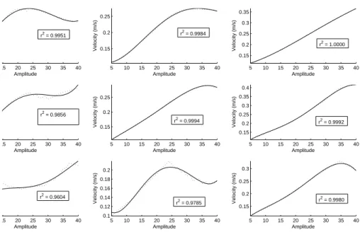
43 5.3. Maintaining the mean velocity 15 20 25 30 35 40 Amplitude 5 10 15 20 25 30 35 40 0.15 0.2 0.25 Amplitude Velocity (m/s) 5 10 15 20 25 30 35 40 0.15 0.2 0.25 0.3 0.35 Amplitude Velocity (m/s) 15 20 25 30 35 40 Amplitude 5 10 15 20 25 30 35 40 0.15 0.2 0.25 Amplitude Velocity (m/s) 5 10 15 20 25 30 35 40 0.15 0.2 0.25 0.3 0.35 0.4 Amplitude Velocity (m/s) 15 20 25 30 35 40 Amplitude 5 10 15 20 25 30 35 40 0.1 0.12 0.14 0.16 0.18 0.2 Amplitude Velocity (m/s) 5 10 15 20 25 30 35 40 0.15 0.2 0.25 0.3 Amplitude Velocity (m/s) r2 _{= 0.9951} r2 = 0.9984 r2 _{= 1.0000} r2 = 0.9856 r2 _{= 0.9994} r2 _{= 0.9992} r2 _{= 0.9604} r2 _{= 0.9785} r2 _{= 0.9980}

Figure 5.4: Speed characterization of the robot for different values ofω and Tswing= 0.9. The plots correspond to the experiments numbered from 1 to 9, in the order from left to right, and from top to bottom. The experiment observations are plotted in a dotted line, while the regression model is plotted in a solid line. The values of the r2_{statistic for each}

and then we can use Newton's method to find a solution for a specific mean velocity

b2×µ+ b3×µ2+ b4×µ3+ b5×µ4− vavg,d+ b1= 0. (5.5)

This is the equation we use to find the amplitude needed in order to maintain the desired velocity, v_avg,d.

The WEBOTS world used in this stage is shown in figure 5.5. The leg was set in motion for 120 seconds, and went through the three different floor types, with the weight of the lift changing in set points in time. The weight started at 1Kg and was changed to 10Kg at the 30s mark, 5Kg at 40s, 1Kg at 70s, 10Kg at 90s, and 5Kg at 110s. The oscillator's amplitude was changed every time the lift mass or the floor type changed, using (5.5), with the regression coefficients corresponding to the experiment which used the current lift mass/floor type combination, and a desired velocity of 0.15 m/s.

5.4

Results

The mean velocity achieved on this stage was of 0.1507 m/s, against the desired 0.15 m/s. Figure 5.6 shows the evolution of the mean velocity of the leg through the whole run. We can see that the mean velocity shows a more or less steady increase until it reaches a value of approximately 0.15 m/s (the desired value) at around 12 seconds of the experiment,and remains almost constant afterwards. The hip oscillator's amplitude changes with each lift mass/floor type change. The floor type changes twice in a short period of time at around 35s and 70s due to the nature of the leg's walking motion swing phase, which as a small

45 5.4. Results

Figure 5.5: Simulated world on WEBOTS, for the second stage. period where the leg first retracts, so it can propel forward afterwards.

20 40 60 80 100 120 t (s)

Chapter 6

Velocity control using an inverse

model

The inverse model approach, introduced in chapter 4, section 4.3, was used in the second stage of this work.

As stated before, and inverse model uses states (s) and outcomes (z) to predict the neces-sary action (u) [5]

u = ˆf−1(s, z), (6.1)

In this approach, the output is the average velocity of each stride of the system's locomotion. The state vector will contain the total displacement of the system's center of mass in the 47

last stride,∆x, and the mean ground reaction force of the system's lower end along the simulated world x axis direction of the last stride, GRFx. The action chosen on this stage is the CPG network hip's swing phase duration, Tswing,hip. The reason to evaluate the system at each stride as to pertain with the periodic nature of the control system. The position of the joints is controlled throughout each stride by the control network output, and while we don't control the position at each simulation time step, we can control the parameters that mold the sinusoidal that will control the system for each stride. As such, we focus on learning the correct parameters for the next stride, to reach the desired speed. This approach is possible, as opposed to the evaluation on a longer time scale that was done in the first stage, because the learning algorithm we used for the inverse model uses incremental and online learning.

The learning algorithm used in this stage was Locally Weighted Projection Regression [41]. This algorithm achieves nonlinear function approximation through the use of various local linear models, that have associated weighting kernels which are used to give each model the correct contribution to the output of a query point. Each model, called receptive field, projects the input vector on the most relevant dimensions to estimate the output vector. This small number of univariate regressions in selected directions is achieved using a mod-ified version of Partial Least Squares, while the receptive fields are learned through local regression. Both this learning steps are done incrementally, which allows the size and shape of the receptive fields to change both during training and during testing, this feature being the main reason this algorithm was chosen for the task.

The inverse model needed to control the system's traveling speed can be described as

49

Figure 6.1: Simulated environment used in the first training and first and second sets of tests for this stage of the work.

where vavgis redefined from the previous chapter. This model was obtained through the use

of LWPR by running the system in a single run, on the simulated environment of Figures 6.1 and 6.2 changing the T_swing,hipparameter at an interval of two strides. The obtained model was then tested on simulated environments with different floor conditions and different lift masses, compared to the training phase. This consists in a training phase with much less data used, compared to the first stage, was well as no training in different floor types and with different lift masses. This was done with the intention of showing the online adaptive capabilities of LWPR.

The simulated environments were the velocity control of the system was tested are showed on Figures 6.1 and 6.3.

Figure 6.2: Simulated environment used in the second training for this stage of the work.

51 6.1. Training in the simulated environment

6.1

Training in the simulated environment

The system was trained in two separate training phases. It was ran in the simulated environ-ments previously mentioned, controlled by a network of two CPGs, implemented through Hopf oscillators. The sinusoidal waves of the output of the x variable of the oscillators are translated into position commands for the actuated joints, resulting in a smooth locomotion. The oscillator's parameters, described in chapter 4, sections 4.2, used for both the training phases were as follows: αhip = ₄₅1 and αankle = ₄₅1, variables that control the speed of convergence for the limit cycle; _µhip = 15× 15 and µankle = 15× 15, where √µ represents the amplitude of the oscillations; the offsets where all set to 0; λ = 0.5, the duty factor, meaning the swing and the stance phases have the same duration; b = 500 controls the alternation speed of the frequency modulation.

The Tswingparameter for the hip's oscillator was the one chosen as the control variable of the learning control approach. The system's velocity is closely related to the period of both phases of the oscillator cycle, as stated on chapter 4. The Tswing of the ankle's oscillator was set as twice the value of that of the hip's oscillator. To evaluate the system's response to various values of Tswing, the system was ran during 135 seconds of experiment, with the first 5 not accounted for, to give time for the oscillator to reach a limit cycle and the system's general locomotion to stabilize. During those 135s, the Tswing was started at 1.085s, reduced to 0.455s at midpoint of the 130s, and again raised to 1.085s by the end of the simulation. The parameter was changed with 0.015s increments, with each change occurring at an interval of two strides of the locomotion.