Growth Accounting and Regressions

(1)

Growth Accounting and Regressions: a new

methodological approach to capital and

technology

VERSÃO DEFINITIVA APÓS DEFESA PÚBLICA

Hugo Miguel Fernandes Morão

Dissertação para a obtenção do Grau de Mestre

Economia

(2

o

_{Ciclo de estudos)}

Orientador: Prof. Doutor Tiago Miguel Guterres Neves Sequeira

(2)

Growth Accounting and Regressions: a new methodological approach to capital and technology

(3)

Dedication

“Truth is treason in the empire of lies.

— Ron Paul, U.S. Representative from Texas

“The best method for estimating the intelligence of a ruler is to look at the men he has around him.

— Niccolò Machiavelli, Italian - Writer | 1469 – 1527

“Gold Is Money, Everything Else Is Credit.

— J. P. Morgan, American - Banker | 1837 – 1913

“I would remind you that extremism in the defense of liberty is no vice! And let me remind you also that moderation in the pursuit of justice is no virtue!”

— Barry Goldwater, U.S. Senator from Arizona

“Speech was given to man to disguise his thoughts.

— Charles Maurice de Talleyrand, French - Diplomat | 1754 – 1838

“I have no trouble with my enemies. I can take care of my enemies in a fight. But my friends, my goddamned friends, they’re the ones who keep me walking the floor at nights!”

— Warren G. Harding, 29th President of the United States

“Never presume that I will not act on my worst instincts.

— Cesare Borgia, Italian - Philosopher | 1475 – 1507

“Should I change my style now? Hmpf... How stupid of me... I already know the answer I am not going to change at all... it would be a crowning achievement of the dumb moves to me to do something like that. A disciplined person knows when needs to control himself. I just gotta stick to the basics.

— Sudō Kyōichi, Team leader of Emperor

(4)

“You can rid yourself of many useless things among those that disturb you, for they lie entirely in your imagination; and you will then gain for yourself ample space by comprehending the whole universe in your mind, and by contemplating the eternity of time, and observing the rapid change of every part of everything, how short is the time from birth to dissolution, and the illimitable time before birth as well as the equally boundless time after dissolution.

— Marcus Aurelius, Roman - Soldier | 121 - 180

“Remember that all we have is ’on loan’ from Fortune, which can reclaim it without our permission—indeed, without even advance notice. Thus, we should love all our dear ones, but always with the thought that we have no promise that we may keep them forever—nay, no promise even that we may keep them for long.

— Seneca, Roman - Philosopher | 4 BC – 65

“But neither a bull nor a noble-spirited man comes to be what he is all at once; he must undertake hard winter training, and prepare himself, and not propel himself rashly into what is not appropriate to him.

— Epictetus, Greek - Philosopher | 55 – 135

(5)

Thanks

I am very grateful to my supervisor Professor Tiago Sequeira for the privilege of having his excel-lent guidance and constant support during this work which certainly without his expertise would not be possible to reach this high level of standards. I am enormously grateful to my friends Es-tefano, André, Zé, Fábio, João, Rúben, Alexandra, Paulo, Cátia, Filipa and my old friend Samuel for all friendship and support during this master’s, also thankful to all teachers that shared their knowledge during the courses. Especially warm thanks go to my parents Vítor and Ana and my brother and sister Marco and Neide for their constant support during this dissertation.

(6)

(7)

Resumo

Foi aplicado um método inédito da contabilidade de crescimento em que assume proporções de factores produtivos variáveis em vez de constantes como é comum. As contribuições da acumu-lação de factores de produção para o crescimento económico tem sido um assunto amplamente analisado e testado na literatura económica. No entanto, várias questões têm posto em causa a fiabilidade dos resultados provenientes das regressões do crescimento tais como a existência de outliers e a de potencial causalidade reversa. O estudo alberga um painel de dados de 101 países entre 1950 e 2015 em que associações entre países e períodos de tempo como choques comuns, características persistentes específicas a cada país e ciclos económicos são analisa-dos e corrigianalisa-dos. A metodologia aplicada contorna várias críticas apontadas ás regressões do crescimento que até ao momento ainda não tinham sido visadas pela literatura mais recente. A evidência mais importante aponta para que a despesa corrente do governo diminua as con-tribuições do capital e trabalho no crescimento mas não que não tenha efeito aparente sobre a produtividade total dos factores (PTF). O comércio externo afecta as contribuições da PTF e do progresso tecnológico enviesado (PTE), porém reduzindo as contribuições associadas á acumu-lação de factores. Além disso, o capital humano diminui a contribuição do PTF, mas aumenta a contribuição do PTE para o crescimento.

Palavras-chave

Crescimento Económico, Contabilidade do Crescimento, Dados em Painel, Contribuições Var-iáveis de Factores, Despesa Corrente, Capital Humano, Comércio Externo, Factores Historica-mente Enraízados, Bootstrapping, Multi-Clustering

(8)

(9)

Resumo alargado

A relação entre as contribuições dos factores produtivos para o crescimento económico é um tema que tem sido amplamente analisado na literatura. Desde Solow (1956) que a contabili-dade do crescimento ganhou lugar na ciência económica para acessar as fontes mais importantes de crescimento económico. Uma das questões mais importantes na explicação do crescimento económico é a importância da acumulação de factores de produção e tecnologia como impul-sionadores da taxa de crescimento económico. Em artigos influentes, Hall and Jones (1999) e Easterly and Levine (2001) concluíram que a fonte mais importante de crescimento é a produtivi-dade total dos factores (PTF) sendo que o primeiro apresentou como explicação as diferenças na PTF são baseadas essencialmente em diferenças institucionais entreas nações. A grande maioria dos artigos que implementam metodologia de contabilidade de crescimento baseiam-se no pressuposto que as contribuições dos factores são consideradas constantes, seguindo aquilo que se conhece como o facto estilizado de Kaldor. No entanto, estudos sobre as proporções de factores feitos como o de Zuleta (2008) concluem que elas variam consistentemente entre os países. Neste estudo, aplicamos a metodologia Zuleta (2012) para obter as proporções da acumulação de capital e tecnologia numa grande variedade de países ao longo de um grande horizonte temporal usando períodos gerados a partir de médias de 5 anos de modo a evitar choques não relacionados com o crescimento de longo prazo. Este trabalho também inova ao incluir o progresso técnico enviesado (PTE) que representa o viés no crescimento a favor dos factores com maior intensidade em capital humano logo mais produtivos. Métodos avançados de econometria em painel são usados para avaliar como a instabilidade, o peso do governo na economia, a abertura ao comércio e o capital humano os afectam. Neste sentido, estamos a ir além da questão central do crescimento económico ‘Por que é que alguns países crescem mais do que outros?’ Na verdade, desejamos perguntar ‘Por que alguns países dependem mais da acumulação de factores ou da tecnologia para crescer?’ Embora possam ser tiradas várias lições dos resultados mais robustos (e recentes) das regressões do crescimento, as razões pelas quais alguns países dependem mais da acumulação de factores ou do progresso tecnológico ainda não foram plenamente comprendidas. Esta é a primeira contribuição desta dissertação: obter uma primeira avaliação do motivo pelo qual os países dependem mais do acumulação de factores, do crescimento da PTF ou da PTE para apoiar o seu próprio processo de crescimento económico. Ao contrário do que acontece em microeconometria, em painéis macroeconómicos as distribuições e as correlações dos erros e das variáveis explicativas representam características especiais dos países e/ou dos períodos em causa. Em termos da forma com as observações estão distribuídas é evidente a presença de outliers dado que eles reflectem a existência de casos de sucesso e os fracassos de políticas económicas, desde sempre foieste um tema relevante para a temática do crescimento em que vários trabalhos referem que os outliers tendem conduzir as regressões levando a resultados significantes quando na realidade não o são bastando apenas pequenas al-terações na amostra para o resultados se modificarem completamente. Segundo, as observações entre si possuem dispersões díspares o que remete para uma natureza distinta da composição das taxas de crescimento de país para país. Fenómenos de correlação ao longo do tempo e de país para país estão presentes nas diferentes variáveis explicativas e nos erros o que reflecte que esses países compartilham certos padrões espaciais como choques comuns e características persistentes que são específicas a cada país, também se verificou que a existência de efeitos tipo ciclo económico em que choques comuns são persistentes no tempo. A adequação dos ix

(10)

estimadores ás especificidades é bem e discutida ao dados do painel. Para o factor capital e progresso técnico foi usado um estimador á la Thompson (2011). Para o factor trabalho foi usado estimador á lá Petersen (2009) e para o progresso técnico enviesado um mais tradicional que é o Arellano (1987). A evidência mais importante revela que o gasto corrente do governo reduz o crescimento dos factores porém não tem efeito sobre a PTF. O comércio externo, no entanto, afecta a PTF e a contribuição do PTE ao mesmo tempo também tende a diminuir a contribuição do capital. Além disso, o capital humano diminui a contribuição da PTF, mas aumenta a con-tribuição do BTC para o crescimento. Determinantes do desenvolvimento mais profundamente enraízados, como a diversidade étnica e a densidade populacional histórica, também afectam a acumulação dos factores, a PTF e a PTE de diferentes maneiras. Por exemplo, a densidade populacional histórica tende a diminuir a contribuição do trabalho, mas aumenta a contribuição do PTE para o crescimento. Além disso, a diversidade étnica tende a elevar as contribuições do trabalho e de PTE, mas diminui a contribuição do capital físico. Finalmente, a temperatura tende a aumentar a contribuição do trabalho no crescimento. Olhando para os resultados de uma perspectiva diferente, a participação de capital diminui devido ao comércio externo, despesa em consumo do governo e à diversidade étnica. A participação do trabalho diminui devido aos mesmos determinantes, mas aumenta com a temperatura e diversidade étnica. A contribuição da PTF aumenta devido ao comércio internacional, mas diminui devido ao capital humano. Fi-nalmente, a contribuição do progresso técnico enviesado aumenta devido ao comércio, capital humano, densidade populacional histórica e diversidade étnica. Entre os diferentes métodos de estimação, um dos resultados mais robustos é o efeito negativo do consumo do governo so-bre as contribuições da acumulação de factores. O nosso trabalho aso-bre vários caminhos para futura investigação. No lado metodológico, oferece uma nova abordagem baseada em méto-dos econométricos recentemente desenvolviméto-dos. Para lidar com aspectos críticos em regressões de crescimento. Do lado dos resultados, destaca-se que diferentes determinantes podem ex-plicar diferentes fontes de crescimento (factores de produção e tecnologia) e que as regressões de crescimento podem ser enganosas quando se tenta explicar o crescimento geral. Uma sug-estão directa para pesquisas futuras é considerar os diferentes determinantes do crescimento dos factores de produção e tecnologia. Essa sugestão inclui o estudo da influência de determi-nantes imediatos do crescimento, como o capital humano e determidetermi-nantes mais profundamente enraizados historicamente, como a temperatura ou a densidade populacional histórica.

(11)

Abstract

We apply a variable shares growth accounting method for 101 countries between 1950 and 2015. Then we estimate regressions for those factor shares and technology using a panel data esti-mator robust to temporary country-wide common shocks, persistent country characteristics, business cycles shocks, reverse causality and high influential observations outliers. This way our applied methodology takes into account the specific features of the data and overcomes most criticisms previously raised on growth regressions, which received only few attention in the economic literature yet. The most important evidence reveals that government current expenditure decreases the factor contribution and has no effect on total factor productivity (TFP). Trade, affects the TFP and the Biased Technical Change (BTC) contributions, decreasing the factor shares. Moreover, human capital decreases TFP and increases the BTC contribution to growth.

Keywords

Economic Growth, Growth Accounting, Cross-Country Data, Variable Factor Share, Total Factor Productivity, Skill-biased Technical Change, Government Expenditure, Human Capital, Trade, Deep-root factors, Multi-Way Clustering, Wild-cluster Bootstrap

(12)

(13)

List of Figures

3.1 Contributions by Income Level (averaged 1950-2015) . . . 7

3.2 Factor Contribution Australia 1950-2015 . . . 8

3.3 Factor Contribution New Zealand 1950-2015 . . . 8

3.4 Factor Contribution Portugal 1950-2000 . . . 8

3.5 Factor Contribution Singapore 1950-2015 . . . 8

3.6 Government Spending share 1950-2015 . . . 9

3.7 Country-specific effects . . . 9

3.8 Trade openness 1950-2015 . . . 10

3.10 Human capital per person 1950-2015 . . . 10

3.12 Guerrila Warfare 1950-2015 . . . 11

3.14 Population density in 1 CE (country region) . . . 11

3.15 Temperature (country region) . . . 12

3.16 Ethnic Diversity (country region) . . . 12

4.1 Diagnostic plot of standardized robust residuals versus robust Mahalanobis distance 18 A.1 Gaussian kernel density estimation. . . 43

A.2 Heteroskedasticity Visual Test . . . 43

A.3 Studentized (jackknifed) residuals. . . 43

A.4 Leverage against squared residual plot . . . 43

A.5 Factor Contribution Spain 1950-2000 . . . 43

A.6 Factor Contribution Denmark 1950-2015 . . . 43

A.7 Factor Contribution Brazil 1950-2015 . . . 44

A.8 Factor Contribution China 1950-2015 . . . 44

A.9 Factor Contribution France 1950-2015 . . . 44

A.10 Factor Contribution South Korea 1950-2015 . . . 44

A.11 Factor Contribution South Africa 1950-2015 . . . 44

A.12 Factor Contribution USA 1950-2015 . . . 44

A.13 Factor Contribution Argentina 1950-2015 . . . 45

A.14 Factor Contribution Canada 1950-2015 . . . 45

A.15 Factor Contribution Denmark 1950-2015 . . . 45

A.16 Factor Contribution Netherlands 1950-2015 . . . 45

A.17 Factor Contribution Africa countries 1950-2015 . . . 45

A.18 Factor Contribution Latin America countries 1950-2015 . . . 45

A.19 Factor Contribution Central,South and East Asia 1950-2015 . . . 46

A.20 Factor Contribution Middle East countries 1950-2015 . . . 46

A.21 Factor Contribution Oceania countries 1950-2015 . . . 46

A.22 Factor Contribution South Asia countries 1950-2015 . . . 46

A.23 Factor Contribution OECD countries 1950-2015 . . . 46

A.24 Factor Contribution Europe countries 1950-2015 . . . 46

(16)

(17)

List of Tables

3.1 List of regions . . . 7

3.2 Descriptive statistics . . . 13

4.1 Langragian multiplier test of independence . . . 16

4.2 Breusch-Pagan and Doornik-Hansen Tests . . . 16

4.3 Pesaran and Wooldridge Tests . . . 16

4.4 Ramsey and Pregibon Tests . . . 17

4.5 VIF and Condition Index . . . 17

4.6 Errors diagnosis sum up . . . 19

4.7 Error and regressors correlation assumptions . . . 19

4.8 Panel robust estimation results . . . 21

4.9 Estimation results with wild-cluster bootstraped SE’s . . . 23

4.10 Estimation results with dummy DK SE’s . . . 24

A.1 List of countries . . . 42

A.2 Variables, Label and Source . . . 42

(18)

(19)

List of Algorithms

1 R Code . . . 37 2 Stata code . . . 39

(20)

(21)

List of Acronyms

UBI Universidade da Beira Interior

OLS Ordinary Least Squares

TFP Total Factor Productivity

BTC Biased Technological Change

GDP Gross Domestic Product

PWT Penn World Tables

CNTS Cross-National Time-Series Data Archive

G-ECON Geographically based Economic data

EU European Union

EZ Euro Zone

WTO World Trade Organization

CE Century

OECD Organisation for Economic Co-operation and Development

AR(1) First Order Autoregression

MA Moving Average

VIF Variance Inflation Factor

RESET Regression Equation Specification Error Test

DK Driscoll-Kraay

VCE Variance-covariance Matrix

(22)

(23)

Chapter 1

Introduction

1 _{Production factor shares and economic growth have been extensively analyzed in the}

liter-ature. With Solow (1956), growth accounting entered into economics science in an effort to identify the most important sources of economic growth. One of the most important issues is the importance of factors of production and technology as contributors to the economic growth rate and income. In influential articles, Hall and Jones (1999) and Easterly and Levine (2001) concluded that the most important source of growth is total factor productivity (TFP). In par-ticular, Hall and Jones (1999) present evidence according to which differences in TFP are based on institutional differences among countries. However, in most of the articles implementing growth accounting methodology, factor shares are assumed constant, following the well-known Kaldor stylized fact for the US. However, factor shares studies made by Zuleta (2008), for ex-ample, conclude that they routinely vary across the countries.

In this study we apply Zuleta (2012) methodology to obtain the shares of capital accumulation and technology across a large cross-section of countries over several years. Then, we use econo-metrics to evaluate how instability, government weight in the economy, openness to trade and human capital affect them. In that sense we are going beyond the important question ‘why do some countries grow more than others?’ In fact, we wish to ask ‘why do some countries rely more on factor accumulation or on technology to grow?’ While several lessons can be taken from the most robust (and recent) results on growth regressions, the reasons why some countries rely more on factor accumulation or on technological change have not been assessed yet. This is the first contribution of this paper: to gain a first assessment of why countries rely more on factor accumulation, TFP growth or biased technical change (BTC) to support their own process of economic growth.

We also deal with common problems affecting the study of the relationship between growth and its determinants, namely the criticism in the literature on the growth regressions literature (e.g. Sala-i Martin (1997)). It is not rare to see cross-country studies tending to disregard heterogene-ity and some possible interdependence across countries (Eberhardt, 2011).2 In our econometric estimations, we deal with heterogeneity, endogeneity, and extreme observations following re-cent contributions for panel data estimations in small samples. First, Nakamura et al. (2017) show that when estimating growth regressions in panel datasets it is crucial to consider both country-specific shocks and worldwide shocks that have mid-term half-life, and serious biases

1

This dissertation was written in X E LA_{TEX using Paulo (2016) template following the principal order nº 49}

/ R / 2010.

2

Many studies simultaneously handle country and time-period effects employing dummies even though this procedure has serious limitations. Both fixed-effects have problems in dealing with complex error structures. Country-dummies do not model accurately the autoregressive process and time-period dummies do not capture some specific country dynamics. Second, the use of dummies restricts the number of covariates that can be used due to collinearity with other regressors and country-dummies inflate the standard errors when the covariates do not vary much across time-periods (see e.g. Thompson (2011)).

(24)

will emerge if we fail to take into account implying e.g. overrejection of the null, which will deceive the researcher by suggesting statistical significance where it does not exist. Second, Thompson (2011) makes a strong case for robust standard errors estimation in panel models where the errors and regressors have both time and country effects and persistent idiosyncratic shocks that affect different countries in different time periods. We use robust standard-error in line with the contributions of Millo (2017). Third, a common concern about growth regressions is the endogeneity bias which in our case is solved by including country-effects that wipe out individual heterogeneity potentially correlated to the regressors. Finally, another of the main criticisms of empirical works using cross-section growth regressions that is usually neglected is that the presence of extreme observations generates weak and dubious economic inference (Easterly, 2005; Kaffine and Davis, 2017). To tackle this problem we integrate in our covariance estimation the Cribari-Neto and da Silva (2011) weighting function, which surpasses the other methods in the presence of very influential observations.

In fact, we think that overcoming those main criticisms raised against the growth regressions methodology is our second contribution to the literature. In that sense, this paper is also re-lated to the contributions of Sala-i Martin (1997); Brock and Durlauf (2001); Durlauf (2005); Ley and Steel (2009). All these papers criticize traditional growth regressions questioning their use-fulness to obtain lessons for the understanding of economic growth or for design policy. Some of them also suggest some ways to improve their inference properties. In this paper we ap-ply alternative econometric approaches developed recently (Thompson, 2011; Cribari-Neto and da Silva, 2011; Yu, 2013; Millo, 2017) to address this issue.

The most important evidence from our empirical exercise reveals that government current ex-penditure (as a ratio to GDP) decreases the factor contribution and has no effect on total factor productivity (TFP), highlighting very important long-run crowding-out effects or Ricardian-like intertemporal effects. Trade, however, affects the TFP and the Biased Technical Change (BTC) contributions, tending to decrease the factor contribution. Moreover, human capital decreases the TFP contributions but increases the BTC contribution to growth. More deeply rooted deter-minants of development such as ethnic diversity and historical population density also affect factor accumulation, TFP, and BTC in different ways. Finally, temperature tends to raise the labor contribution and decrease the TFP contribution.

The structure of the paper is the following. In chapter 2 we review the relevant literature. In chapter 3 we show how we applied the growth accounting methodology and built the variables. In chapter 4 we explain and present the growth accounting methodoloy for the factors accumu-lation and technology obtained in the previous chapters and present our results. In chapter 5, we conclude.

(25)

Chapter 2

Literature Review

Although the doubt about the constancy of shares was already expressed by Keynes (1939) and Solow (1957), most of the field researchers continue to allege that factor shares are constant, as is the case of Brown and Weber (1953) and this evidence has been restated by Kaldor (1961), as a stylized fact of Macroeconomics. This stylized fact has been extensively used in both exogenous and endogenous growth theories, without much questioning of its empirical validity over years and countries, and especially in growth accounting aplications (Barro, 1999).

Kahn and Lim (1998) show evidence that the income shares of equipment, production workers and non-production workers have clear trends. In Blanchard (1997) it is observed that the share of labor decreases in Europe after the 1980’s and the reason for the decline is pointed out to be the technological bias. Some other authors calculate the income share of reproducible factors, like human and physical capital, and non-reproducible factors and contend that the latter is correlated positively with the income level (Krueger, 1999; Caselli and Feyrer, 2007).

Despite the interest in biased technological change raised by the seminal work of Acemoglu (2002), there have been few attempts to correct the standard measure of total factor of pro-ductivity (TFP) according to the existence of biased technological change. In the US there is some evidence that technology has favored skilled workers since the 1980s in manufacturing (Mallick and Sousa, 2017). Sturgill (2012) decomposed the labor’ share into reproducible and non-reproducible components with cross-country estimates, and finds that the labor’ share is negatively correlated with output per worker.

Some economists draw attention to the ratio between capital and labor measured in efficiency units, which have remained steady since the 1980s. Bental and Demougin (2009) propose a model that predicts a decreasing ratio between labor in efficiency units and capital, falling wages per efficiency units and increase in labor productivity.

Sturgill (2014) analyzes the development accounting differently from the standard baseline, incorporating natural capital and treating factor shares as variables instead of constant param-eters using translog multilateral indices of outputs, inputs and productivity. The results reveal that the correction for the mismatch between physical capital and its share, which is the weight assigned to physical capital input in development accounting, reduces the variation in output per worker.

Since the seminal article from Barro (1991), growth regressions have seen exponential applica-tions trying to assess the most important determinants of economic growth. The so-called Barro regressions highlighted positive factors associated with growth such as investment in physical and human capital, openness to trade and negative factors associated with growth such as the

(26)

government weight in the economy and distortions in the market (e.g. the black market ex-change rate premium). Additionally, Easterly and Rebelo (1993) positively associated public investment in transport and communication with growth. Corruption was found to deter invest-ment (e.g. Ades and Di Tella (1997)). Macroeconomic factors like inflation and budget deficits also have a role in growth by reducing both capital accumulation and TPF growth as in Fischer (1993). Financial markets development has been associated with growth (see Levine (1997) and Levine (2005) for important surveys). More institutional, historical and geographical factors as-sociated with growth have been highlighted by Easterly and Levine (2003). However, outliers are the main driver of many big policy effects exposed in growth regressions because they typ-ically represent very ‘bad’ policies (Easterly, 2005). As stated in Bertrand et al. (2002), only a small number of empirical studies using panel methods have employed clustered standard errors to deal with that problem.1

1_{Please see the technical problems pointed out to the growth regressions methodology discussed in the}

Introduction.

(27)

Chapter 3

Growth Accounting Methodology

In this section, we analysed the panel data collected from 1950 to 2015 for 101 countries A.1. The only selection criteria used was the data availability for the longest time span. All variables are quinquennial to avoid unrelated short run oscillations. The samples were collected from very well-known databases like PWT, G-Econ and CNTS. The econometric methods were executed using R Studio by R Development Core Team (2017) and Stata 14 by StataCorp (2015). 1

We also used Excel by Microsoft Corporation (2016) for some charts. The new Zuleta (2012) approach creates 4 growth shares assuming, contrary to the usual growth accounting method, variations in capital and labor shares. The outcome variables come in contributions which are Capital, Labor, Solow Residual and Biased Technological Change.

3.1 Applying the Growth Accounting Methodology

First, the central concept in the model is the production function with all the standard assump-tions,

Yt= AtF (θkKt, θlLt) (3.1)

where Ytis Output-side real GDP at current PPPs (in mil. 2011US$), Ktis Capital stock at current

PPPs (in mil. 2011US$), and Ltis Number of persons engaged (in millions). These raw variables

were extracted from PWT. The factor shares vary over time so the relative abundance of factors becomes extremely important and, therefore, it is required to have accurate measures of capital and labor, θkand θlare used as parameters for this reason. The economy is labor abundant when θlLt≥ θkKt.

The annual compound growth of output rate is gy=

( Yt Yt−1 )(1/5) − 1 Differentiating (3.1) we have, gy = [ ga+ αtgk+ (1− αt)gl+ ∆αtln ( θkKt θlLt )] (3.2)

The Ytelasticity with respect to capital is αtand (1− αt)is the elasticity of output with respect

1_{The Stata and R code are available in A.1 and A.2.}

(28)

Growth Accounting and Regressions: a new methodological approach to capital and technology to labor. gk= ( Kt K_t−1 )(1/5) − 1 gl= ( Lt L_t−1 )(1/5) − 1 St= gy− (αtgk+ (1− αt)gl) (3.3)

The Solow residual of Eq.(3.3) is the Stvariable. The Solow residual from (3.2) and (3.3) also

contains the skill-biased technological change (BTC).

St= ga+ ∆αtln ( θkKt θlLt ) (3.4)

Using this expression ˜St= St− ∆αtln

(

Kt Lt

)

we can rewrite (3.4) this way,

˜ S = ga+ ∆αtln ( θK θL ) (3.5)

The subsequent equation can be estimated ˜ S = C0+ C1∆αt+ τt (3.6) where ga = C0+ τtand C1= ln ( θK θL ) .

3.2 Graphical Analysis

3.2.1 By Country Region

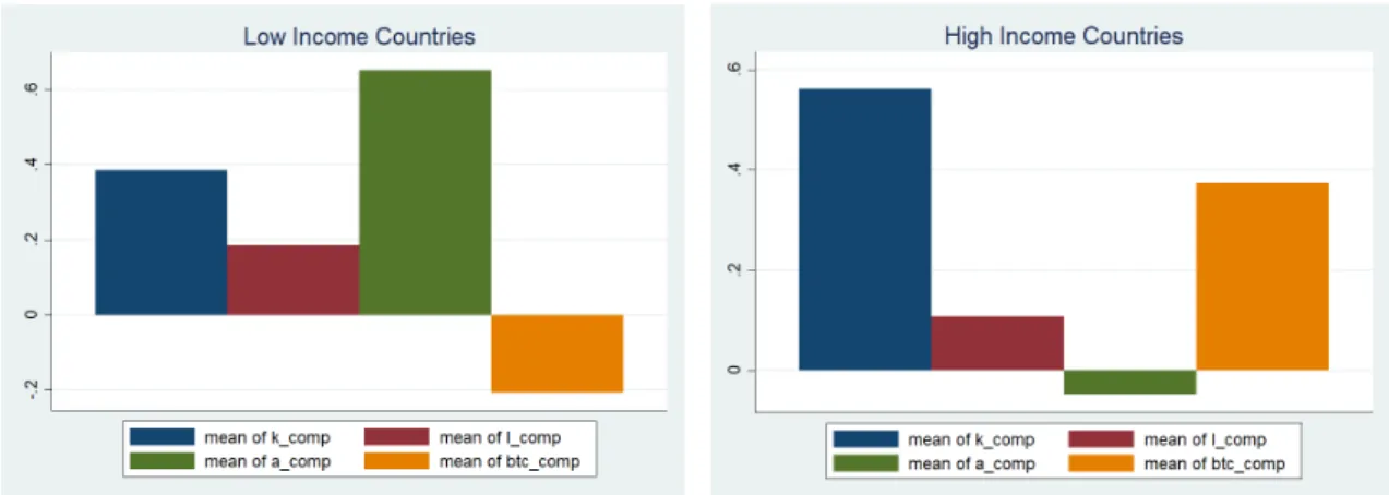
In this section, we are going to analyse the contributions for the growth decomposition: • K_comp - Capital Contribution

• L_comp - Labor Contribution • A_comp - Productivity Contribution

• BTC_comp - Biased Technological Change Contribution

As an example of the data obtained we show a figure 3.1 for low and high income countries.2

2

Figures for other groups of countries are available on appendix Additional Figures A.4.

(29)

Table 3.1: List of regions

label Region

h/l high/low countries africa africa countries lat latin america countries

casia central, south and east asia countries meast middle east countries

oceania oceania countries

sasia southeast and asian tigers countries oecd oecd countries

europe non-oecd european countries

Figure 3.1: Contributions by Income Level (averaged 1950-2015)

Note: Bar charts created using Stata. Note: Bar charts created using Stata.

Lower income countries obtained their growth most gains from productivity growth and capital accumulation. The negative biased tech may be explained by a brain drain effect that moved high productive workers to rich countries.

In rich countries, we can check on of the main problems of nowadays which is a stagnation of productivity and the improvements occurring from the labor and capital contributions as well as a positive biased technical change contribution.

3.2.2 By Individual Countries

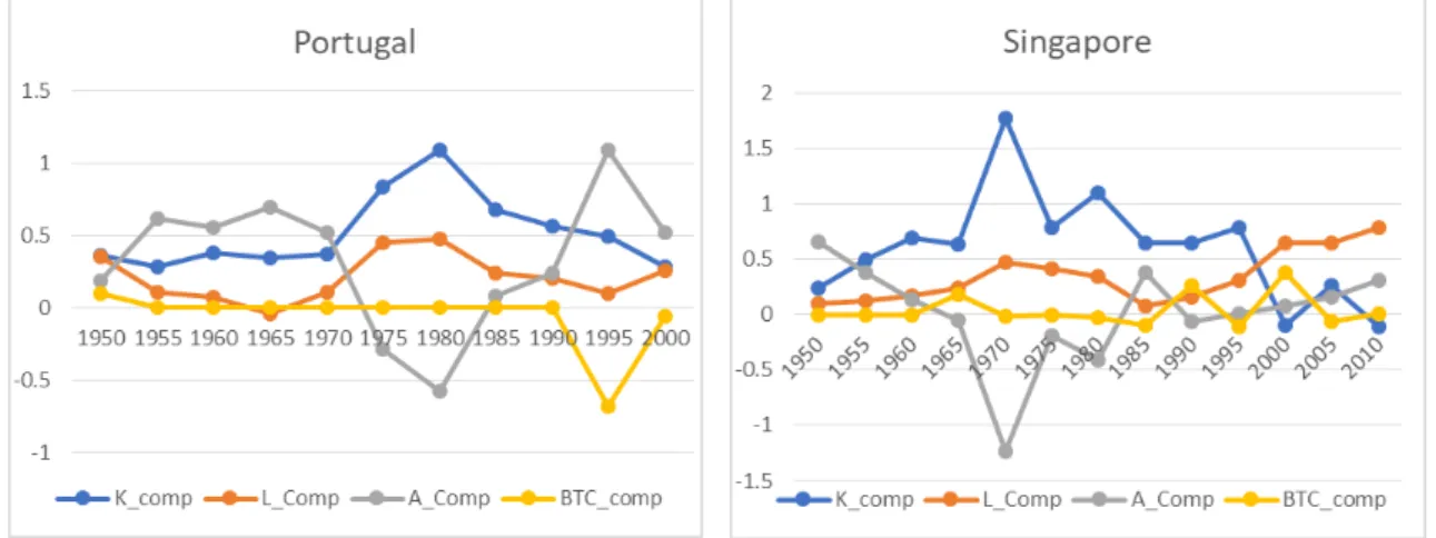
We took 4 from the sample countries (Australia, New Zealand, Portugal and Singapore).

(30)

Note: Line charts created using Excel.

Figure 3.2: Factor Contribution Australia 1950-2015

Figure 3.3: Factor Contribution New Zealand 1950-2015

Australia is a vibrant free-market economy with an impressive performance without a recession for more than 25 years. After the internationalization of the economy in 1980s the capital converged with labor with a good TPF growth. New Zealand largely liberated the economy in 1980s and 1990s which we can see on build-up of capital and labor and after a high productivity labor rise.

Figure 3.4: Factor Contribution Portugal 1950-2000

Figure 3.5: Factor Contribution Singapore 1950-2015

Portugal is an EU country that needs an urgent economic policy adjustment. 1950s and 1960s were a great period of expansion of the Portuguese economy with greater productivity improve-ment. Singapore is one of the world’s most well-off nations that is characterized by a highly educated workforce and solid legal environment. Singapore shows a very interesting trend while financialization expands his labor contribution grows as well. As expected each country expe-rienced different contributions of each factors, biased technical change and TFP depending on different each historical period. For example, capital accumulation tend to be more important in Australia, New Zealand and Singapore and TFP is more important in Portugal namely until the 1970s.

(31)

3.3 Variables and Data

3.3.1 Regressors

3.3.1.1 Government current expenditure

Economic growth is inversely related to the government current expenditure (as a ratio to

GDP) (csh_g) meaning that lower government consumption enhances growth Barro (1997). This

relationship is strong specially in developing countries which goes in line with Pritchett and Ai-yar (2015) because only the richer countries tend to be able to afford for large governments. The contribution of the government expenditures or debts to growth has been particularly con-troversial after the now famous contribution of Reinhart and Rogoff (2010). However in most growth regressions, the government current expenditure (as a ratio to GDP) appear with a neg-ative and significant sign. With our results we will be able to tell which contribution of growth this (an the other) variables is affecting more. In this case, from where comes the negative sign if it exists. The panel data for this variable was extracted from PWT. We can see a rising trend until mid-eighties coinciding with big deficits and inflation period and afterwards a declining since then specially on the top values.

Note: Scatterplot drawn using Stata.

Figure 3.6: Government Spending share 1950-2015

Note: Scatter created using Stata command twoway scatter.

Figure 3.7: Country-specific effects

We can see a rising trend until mid-eighties coinciding with big deficits and inflation period and afterwards a declining since then specially on the top values.

3.3.2 Trade openness

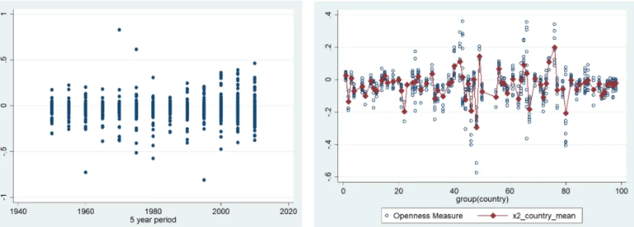
Trade openness (trade) is a openness measure which is obtained by summing exports and

im-ports shares. The relationship between openness and economic growth has been regarded as positive by the literature (Dollar (1992), Frankel and Romer (1999) and Yanikkaya (2003)). In developing countries increased trade openness will not increase wage rates directly and may

(32)

produce declines in real wages as increase distribution across wages, while in developed coun-tries, wage earner will in general gain in medium run with increased trade, with wage dispersions not increasing and probably decline as result openness Majid (2004). The worldwide openness was stagnant until the early nineties when then started to grow caused by expansion of WTO deals.

Figure 3.8: Trade openness 1950-2015

3.3.3 Human capital

In general, and despite some initial controversy (Benhabib (1994)), the most recent empirical literature confirms that Human capital (hc) is positively related to growth (Cohen and Soto (2007); Sunde and Vischer (2015); Teixeira and Queirós (2016)). Human capital in regions with high physical capital tend to have higher incomes for all workers (see e.g Mulligan and Sala-i Martin (1997)). The educational attainment rose from 9 years to 12 years and that explains why human capital is steadily growing.

Figure 3.10: Human capital per person 1950-2015

(33)

3.3.4 Guerrila warfare

Guerrila warfare (gwar) is used as a proxy for political and social instability as higher degrees of

instability are correlated with lower growth rates (Alesina et al., 1996), because it also affects in lowering the rates of overall productivity growth as pointed out by Aisen and Veiga (2013). We have seen an increase of violence till the 70’s and a significative lowering but in the last period we have explosive growth occurred provoked by recent events in Iraq, Nigeria and Ukraine.

Figure 3.12: Guerrila Warfare 1950-2015

3.3.5 Deeply rooted variables

Additionally, we have included 3 time-invariant regressors that improve the explanatory power by adding some geographical factors into account. Ashraf and Galor (2012) show that Population

density in 1 CE (pd1) embody some and significant economic development effects for countries

that have long expanse of time. The Middle East and Central Asia were the regions with higher density because the first big civilizations started there.

Note: Bar chart created using Excel. Y -axis measured in pop/km2

Figure 3.14: Population density in 1 CE (country region)

(34)

Some literature examined the association between average Temperature (temp) and aggregate economic variables using panel data. The main relationship found was a reduced economic growth rates and a lower level of output but the effects are only relevant in poor countries. Dell et al. (2012) Regions near Tropics have naturally higher temperatures average.

Note: Bar chart created using Excel. Y -axis measured in ºC.

Figure 3.15: Temperature (country region)

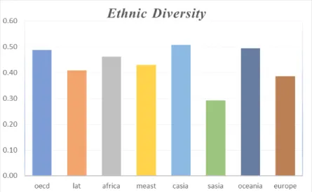
Ethnic Diversity (ethnic) tend to lower a country’s economic growth rate because higher levels

of ethnic fractionalization are related with unstable democracies Easterly and Levine (1997) and Alesina et al. (2003).

Central Asia and OECD are the economic regions with higher ethnic fractionalization.

Note: Bar chart created using Excel. Y -axis measured in %.

Figure 3.16: Ethnic Diversity (country region)

(35)

3.4 Descriptive Analysis

The raw variables were transformed using a cubic root transformation that fits better for data with zeros and negative numbers, and the share data we consider as dependent variables – see e.g. Cox (2011). The descriptive statistics (see Table 3.2) show that we have a very diversified unbalanced panel of countries. More than 70 countries with thirteen 5-years period make this a very good sample. The panel data for csh_g, trade and hc was extracted from Penn World Tables 9.0 (PWT) from Feenstra et al. (2015), gwar from databanks database (cross-national time-series data archive – CNTS, Wilson (2017)) and temp, pd1 and ethnic from Geographically based Economic data (G-Econ) from Nordhaus and Chen (2006). 3

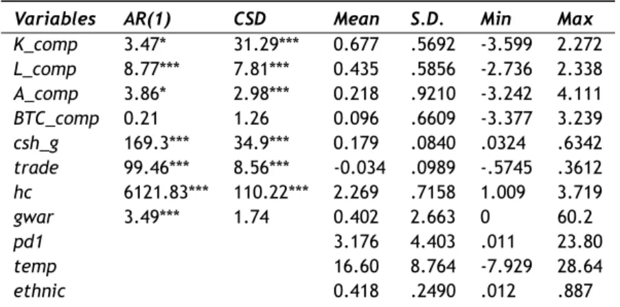
Table 3.2: Descriptive statistics

Variables AR(1) CSD Mean S.D. Min Max K_comp 3.47* 31.29*** 0.677 .5692 -3.599 2.272 L_comp 8.77*** 7.81*** 0.435 .5856 -2.736 2.338 A_comp 3.86* 2.98*** 0.218 .9210 -3.242 4.111 BTC_comp 0.21 1.26 0.096 .6609 -3.377 3.239 csh_g 169.3*** 34.9*** 0.179 .0840 .0324 .6342 trade 99.46*** 8.56*** -0.034 .0989 -.5745 .3612 hc 6121.83*** 110.22*** 2.269 .7158 1.009 3.719 gwar 3.49*** 1.74 0.402 2.663 0 60.2 pd1 3.176 4.403 .011 23.80 temp 16.60 8.764 -7.929 28.64 ethnic 0.418 .2490 .012 .887

Note: K_comp , L_comp , A_comp and BTC_comp are in cubic roots. H0of Pesaran (2015)

Test: Variable is cross sectional independent. H0 of Wooldridge (2002) Test: Variable

follows an AR(1) process. *** p < 0.01, * p < 0.1. The Stata commands xtsum, xtcd2 and xtserial were used to reach the table. There are 719 observations in the sample, covering 71 countries, with a T-bar of 10.127.

3_{For a better view on variables, sources and reference see the appendix Additional Tables A.2.}

(36)

(37)

Chapter 4

Econometric Methodology

4.1 Model Specification

A panel regression is the main method used to analyse two dimensions (country, period). Con-sider the following panel regression

yit≡ σ + vtγ + zitψ + εit≡ X′β + ε (4.1) with, βK,1=    σ γ ψ    (4.2)

yit is the dependent variable, the production factor component or tecnology, X is a vector of

covariates, β is an unknown coefficient vector. εit is a vector of errors terms which can be

heteroskedastic but with zero conditional mean, thus E(εit|xit) = 0. Index i refers to

country-level observations and t to periods where i=1, ... ,N countries observed over t=1, ... ,T periods. The equation (4.2) error term εit and the regressand yit contain three components: εi and xi

represent country-specific effects. ftand gtare both vectors of autocorrelated common factors

that follow an AR(1) process. ϕi and δi represent vectors of idiosyncratic factor sensitivities

that follow N (0, 1). ωitand ξitare the idiosyncratic errors.

εit= εi+ ϕift+ ωit and xit= xi+ δigt+ ξit (4.3)

If ft is uncorrelated across time periods we are in presence of time effects but when ft is

persistent we have both time-period effects and persistent common shocks.

4.2 Assessing assumptions

The error term will probably include unobserved components like country-specific effects and business-cycle shocks that are common and persistent that affect all countries. Checking for eventual violations on assumptions is vital for a good estimation in a heterogeneous panel given their sensibility of usual panel estimator if some of the assumptions are violated a robust stan-dard errors estimator will be required. To that end, we performed a set of tests on stanstan-dardized residuals.

(38)

4.2.1 Specification Tests

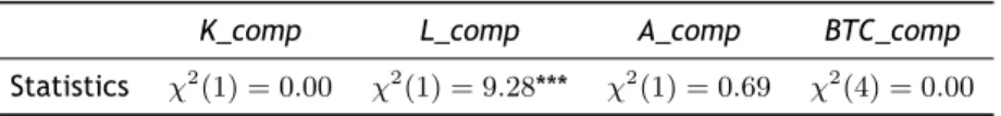
Table 4.1: Langragian multiplier test of independence

K_comp L_comp A_comp BTC_comp

Statistics χ2_{(1) = 0.00} _χ2_{(1) = 9.28***} _χ2_{(1) = 0.69} _χ2_{(4) = 0.00}

Note: *** p < 0.01. H0of Breusch and Pagan (1980) Test: V ar(u) = 0. The Stata command

used was xttest0.

The Langragian multiplier test of independence was performed to verify if the variance across countries is 0. H0 is rejected for L_comp which means that a random effects estimation is the

correct approach for all the others a pooled estimation is the best option.

4.2.2 Distribution of model errors

Table 4.2: Breusch-Pagan and Doornik-Hansen Tests

Homoskedasticity Normality Statistics F (1, 717) = 892.932*** χ2(2) = 1021.003***

Note: *** p < 0.01. Tests executed for K as Dependent variable.H0of

Breusch and Pagan (1979) Test: Constant variance. H0of Doornik and

Hansen (2008) Test: Normality of residual term. The Stata commands used were hettest and mvtest.

We assess the violation of one of main assumptions of OLS estimation that is the normality of the residuals non-normal errors distorts p-values and confidence intervals. The Gaussian kernel and other normality tests also show the same problem. 1

The existence of heteroskedasticity was checked using BP test enhanced by a Wooldridge (2013) F-statistic version that drops the normality assumption. Using the rejection of H0and a visual

assessment2_{we can conclude that the residuals suffer from heteroskedasticity. Heteroskedastic}

residuals require robust standard errors estimation.

4.2.3 Correlation of model

Table 4.3: Pesaran and Wooldridge Tests XXXXX

XXXXX

Equation

Test Spatial Correlation

N (0, 1) Serial Correlation F (1, 70) K_comp 11.347*** 2.915* L_comp 1.237 8.746*** A_comp 3.592*** 3.843* BTC_comp -0.553 0.217

Note: *** p < 0.01, * p < 0.1. H0of Pesaran (2015) Test: Errors are cross

sectional independent. H0of Wooldridge (2002) Test: Errors do not follow an

AR(1) process. The Stata commands used were xtcd2 and xtserial.

1_{see appendix Additional Figures A.1 for visual confirmation.} 2

see appendix Additional Figures A.2 for visual confirmation.

(39)

The Cross-Dependence test detected cross-sectional dependence which originating some com-plications derived from omitted-variables bias when the regressors are correlated with the un-observed common factors Pesaran (2006). This type of correlation may appear when countries or regions share common shocks Eberhardt (2011). The literature identifies two types of depen-dence when there is global wide interdependepen-dence in the panel – see e.g. Moscone and Tosetti (2010) and spatial dependence – see e.g. Anselin (2001). Goverment consumption, Human cap-ital and Trade have relevant correlated common shocks between cross sections. To check the existence of a AR(1) process in the errors terms a Wooldridge (2002) Test was performed and confirmed the existence of autocorrelation.

4.2.4 Assessing model structure

First, we test the proposed model for omitted and redundant variable bias.

4.2.4.1 Omitted and Redundant Variable Bias

Table 4.4: Ramsey and Pregibon Tests

Omitted Variables Redundant Variables Statistics F (3, 708) = 1.42 N (0, 1) =−0.39

Note: Tests only executed for K as Dependent variable. H0 of

Ramsey (1969) RESET test: model has no omitted variables. Pregi-bon (1980) Test: Hatsq p > 0.10. The Stata commands used were

ovtestand linktest.

The RESET Test check if we omitted some relevant variable in the specification process, which was not the case. Linktest is a specification test that verify the existence of redundant variables that can warm the quality of the estimation by biasing the regressors, which also validate our specification.

4.2.4.2 Multicollinearity

Table 4.5: VIF and Condition Index

Mean VIF Condition Number

Value 1.35 2.62

Note: Tests only executed for K as Dependent variable. The Stata command used was collin.

Second, Multicollinearity might be problematic when the VIF and condition number are bigger than 10 because it means that some regressors are closely correlated to one another’s biasing the standard errors, distorting confidence intervals and providing less reliable probability values. The absence of multicollinearity is supported with very low conditions numbers and VIF.

(40)

4.2.5 Important group of observations

In literature, the first concerns about the unreliableness of the method of ordinary least squares (OLS) in presence of outliers came from Edgeworth (1887). The OLS estimation intends to min-imize the squares of the error terms (εi).

min J = n

∑

i=1

ε2_i (4.4)

Rousseeuw and Leroy (2003) explain that some of them the vertical outliers and bad leverage points are particularly problematic. Vertical outliers aff ect the estimated intercept since the observations have outlying values for the residuals whereas bad leverage points are observations that equally have outlying values but are also far away from the regression line.

We used a graphical tool made by Rousseeuw and van Zomeren (1990) to check them, which is created by plotting, on the Y -axis, the robust standardized residuals, de ned as ri/ˆσS, with ˆθS

being a measure of dispersion robust against extreme values making the residuals less sensitive to these values, proposed by Rousseeuw (1984) for measuring the outlyingness in the fitted regression. On the X-axis is plotted the Mahalanobis (1936) distance that measures outlyingness of the explanatory variables. There are some ways to measuring robust Mahalanobis distance but the most robust that we used is the algorithm proposed by Rousseeuw and Van Driessen (1999) using a minimum covariance determinant. We set the limits proposed by Verardi and Croux (2009), where outside the observations are measured as outliers.

• y dimension, between−2.25 and +2.25. • x dimension,√χ2

p, 0.975.

Figure 4.1: Diagnostic plot of standardized robust residuals versus robust Mahalanobis distance

Note: The outliers are flagged with red numbers. Scatterplot drawn using Stata commands mcd and sregress.

(41)

This plot shows that we have some outliers in our dataset, which means that leverage points need to be accounted. Another two visual test using Studentized residuals A.3 and the leverage statistic A.4 reach out to similar conclusions. Table 4.6 summarizes for each of the dependent variable the diagnostic summary and consequently the necessary care to take in each of the regressions presented below.

Table 4.6: Errors diagnosis sum up

Panel SEs need to be robust against

K_comp overleverage, arbitrary heteroskedasticity, within-panel autocorrelation and

cross-panel autocorrelated disturbances.

L_comp overleverage, arbitrary heteroskedasticity and contemporaneous cross-panel correlation.

A_comp overleverage, arbitrary heteroskedasticity, within-panel autocorrelation and

cross-panel autocorrelated disturbances.

BTC_comp overleverage and arbitrary heteroskedasticity.

Note: Arbitrary heteroskedasticity is tested in 4.2, overleverage and outliers were checked in 4.1, within-panel autocorrelation and cross-panel autocorrelation is tested in 4.3.

4.3 Robust Estimation

As a result of the last section results we need to address the violation of distribution and cor-relation of errors assumptions to assure the validity of statistical inference. In the presence of assumptions violated, we use some alternative ways to compute covariances matrix estima-tors in order to obtain robust standard errors. We made three error correlation assumptions. First, εit have country-effects when εit is correlated across time periods for a specific country E(εitεik|xit, xik) ̸= 0. Second, time-period effects are present at some moment in time there

is correlation beetween countries, E(εitεjt|xit, xjt) ̸= 0. Lastly when, E(εitεjk|xit, xjk) = 0if i̸= j and |t − k| > L, we are in presence of persistent common shocks that disappear after L

lags.

Table 4.7: Error and regressors correlation assumptions

Errors Regressors

K L A BTC z1 z2 z3 z4 Country-Effects X X X X X X X X

Time-Effects X X X X X X X

Persistent common shocks X X X X X

S.E. type ϑ ϱ ϑ ϖ – – – –

Notes: ϑ stands for Thompson (2011) standard-errors; ϱ stands for Petersen (2009) standard-errors and ϖ for Arellano (1987) standard errors which is consistent with the information summarized in Table 4.6.

Multi-way clustering was firstly described by Petersen (2009) and generalized after in Cameron et al. (2011) Using the formula with the assumptions defined above

ˆ

VDouble= ˆVCountry+ ˆVP eriod− ˆVW hite (4.5)

where, VˆCountry= ˆH−1 ∑N i=1(ˆciˆc′i)H−1 VˆP eriod,l = ˆH−1 ∑T t=l+1(ˆstsˆt−1)H−1 19

(42)

Growth Accounting and Regressions: a new methodological approach to capital and technology ˆ VW hite,l= ˆH−1 ∑N t=l+1 ∑T l=1(ˆuitˆu′i,t₋₁)H−1 ˆ

VP eriod,0is the traditional formula for clustered SE’s by Period. ˆVW hite is the common OLS SE’s

robust to arbitrary heteroskedasticity. ˆVW hite,land ˆVP eriod,lcorrect for persistent common shock

across panels.

Based on previous works Thompson (2011) upgraded the double-clustering with kernel-robust inference to manage business cycles shocks that disappear after some L periods.

ˆ

VDouble,L_|w= ˆVCountry+ ˆVP eriod+ L

∑

l=1

( ˆVP eriod,l+ ˆVP eriod,l′ )− ˆVW hite− L

∑

l=1

( ˆVW hite,l+ ˆVW hite,l′ ) (4.6)

K_comp and A_comp panels errors and regressors display similar time and country effects which

is when the double clustering matters the most. By clustering on country we produce SE’s and statistics robust to autocorrelated within-panel disturbances and combining a kernel-based HAC with period clustering we correct for autocorrelated across-panel disturbances. L_comp common correlated disturbances are corrected by clustering period and by country – we use the Petersen (2009) standard-errors. For BTC_comp panel double clustering is not required, so we can get the right β by clustering on country – we use the Arellano (1987) standard-errors. Additionally, we tune the variance-covariance matrix to account for the presence of overlever-age points. Also some specifications related with HAC inference are done for K_comp and

A_comp . This affects all the dependent variables and is explained in the following sub-sections.

4.3.1 Overleverage and Heteroskedasticity-Robust inference

A weighting function is used to control the effects of high leveraged observations on the calcu-lation of the covariance

ωt= (1− hi) −δi

2 , δ_i = min(4, h_i/h) (4.7)

where hi = Xt′(X′X)−1Xi are the diagonal components of the H = X′(X′X)−1X′, h is their

mean and δiis exponential discounting factor that is truncated. Cribari-Neto and da Silva (2011)

discuss in detail the effects of these choices and why the HC4 method is better than the bias-correcting HC2 or pseudo-jackknife HC3 proposed in MacKinnon and White (1985) to cope with the presence of influential observations.

4.3.2 Kernel-robust inference

The optimum number of lags is 2 which was calculated Newey and West (1994) lag selection for-mula the number of lags is reasonable taking into account the fact that we use 5-year averages.

m(T ) = f loor[4(T /100)2/9] (4.8)

(43)

The Newey and West (1987) kernel smoother function with linearly decaying weights based on HAC inference was employed.

ωℓ= ℓ

1 + L (4.9)

4.3.3 Panel robust estimation results

Using the specifications mentioned in the previous sections the output came as follows. 3

Table 4.8: Panel robust estimation results hhhhhhh

hhhhhhhhh

Regressors

Dependent Variable

K_comp (1) L_comp (2) A_comp (3) BTC_comp (4)

csh_g -0.841*** -0.799** -0.26 0.321 (0.211) (0.248) (0.366) (0.283) trade -0.45*** -0.225 0.413* 0.51*** (0.061) (0.151) (0.245) (0.181) hc 0.05 0.008 -0.224** 0.116*** (0.067) (0.054) (0.102) (0.042) gwar -0.002 -0.004 0.024 -0.011 (0.074) (0.028) (0.137) (0.108) pd1 -0.001 0.01 -0.002 0.017*** (0.003) (0.006) (0.006) (0.005) temp 0.001 0.005 -0.016*** 0.0017 (0.005) (0.003) (0.006) (0.003) ethnic -0.201*** 0.296** -0.182 0.124 (0.071) (0.091) (0.11) (0.112) Constant 0.765*** 0.296* 1.127*** -0.337** (0.241) (0.179) (0.397) (0.157) Wald F (7, 711) 3.349*** 2.028** 2.68*** 3.097***

Method Pooled Random Pooled Pooled

Note: Regressors are defined in the first column of the Table. Dependent Variables are defined in the first row of the Table. Values in parentheses below the observed coefficients are the Thompson (2011) two-way cluster and kernel-robust SE’s (1 and 3), Petersen (2009) two-way clustered-robust SE’s (2) and Arellano (1987) one-way cluster-robust SE’s (4). Level of significance: *** for p-value > 0.01, ** for > 0.05, * for > 0.1. To reach the results we used R package plm created by Croissant et al. (2017). For (1) and (3) equations we applying a block building process which was built using the commands vcovSCC and vcovHC. Equation (2) used the command vcovDC and (4) the vcovHC. All 4 equations use Cribari-Neto and da Silva (2011) HC4 weighting function. (1 and 3) and Newey and West (1987) kernel-smother with 2lags.

From the analysis of Table 4.8 we can note that the physical capital contribution is strongly in-fluenced by the government share in the economy as well as by trade and ethnic diversification. This indicates a potentially strong crowding-out effect in the long run that can be associated with intertemporal Ricardian effects on the decision of investments when agents expect higher taxes in the future. This also indicates that the usually negative and significant sign of govern-ment expenditures on growth regressions come from the physical capital source of growth. The fact that trade is negatively influencing the physical capital contribution may be explained by an infant industry argument and an explanation why openness is not always significant in growth regressions. This also has some support in the literature. For example Madsen (2009) showed that openness is independent of economic growth in much of history but is clearly positively

3

The algorithm used to reach the results is on appendix R code A.1.

(44)

associated with growth when technology is taken into account. This is exactly what our results seem to support, as trade has a positive and highly significant influence on both total factor productivity and biased technical change contribution of growth. Moreover, economic theory also has shown that in some conditions protectionism may increase welfare (see e.g. Tuinstra et al. (2014)). Finally, ethnic diversity has a highly negative effect on the physical capital con-tribution of growth, which is very much consistent with the empirical literature as in Easterly and Levine (1997) and Alesina et al. (2003).

Interestingly, the government share in income also has a negative effect on the labor share which reinforces our argument toward an intertemporal Ricardian effect in this case on the labor/leisure decisions. Additionally, ethnic diversity appears with a positive effect on the labor contribution, which highlights its potential positive effect on human capital and labor adaptability on the labor market, which also has some support in recent empirical contributions from Hoogendoorn and van Praag (2012) and Maestri (2016). This also indicates that the negative effect that ethnic diversity can have on overall economic growth may come from the investment in physical capital and not in the labor market. The remaining most important results are the significantly negative effect of human capital in the TFP contribution and positive effect in the BTC contribution and a positive effect of historical population density in the BTC contribution. On the one hand, negative effects of human capital in TFP are somewhat unexpected and can be obtained through high duplication effects (see e.g. Jones and Williams (2000)), or complex-ity effects which may lead to negative scale effects (see e.g. Sequeira et al. (2016)). On the other hand, positive effects of human capital on the biased technical change contribution is an expected result, as human capital is more adapted to work with new investments and thus con-tribute to a bias toward capital. Additionally this can be a direct consequence of the positive effect of human capital in wages of the more qualified which may lead to an increase in the capital-labor ratio (Acemoglu (2002); Violante (2012)). The positive effect of historical popu-lation density in the biased technical change contribution is an interesting effect in line with recent evidence that historically determined investments have influence in today’s economic activity (e.g. Dalgaard et al. (2018)). In particular this means that historically more developed regions or countries tend to favor physical capital nowadays, suggesting a channel through which historical persistence of development can occur, i.e., through biased technical change. Finally higher temperatures seem to decrease TFP, suggesting a channel through which temperature (and climate change in general) may affect growth (as shown by e.g. Dell et al. (2012)).

4.3.4 Robustness

Thompson (2011) makes a strong case for double clustering in multivariate regression in which some regressors vary by time and some vary by country but sometimes the most robust method may not be the best option. Cameron et al. (2008) propose a wild-cluster bootstrap low asymp-totic requirement that comes is an easy and very robust check even when the cluster number is midsized. Wild bootstrap as first described in Wu (1986) and further in studies Liu (1988) and Mammen (1993) improved the robustness of bootstrap in presence of heteroskedastic errors. Another popular option is pairs bootstrap that resamples the regressand and regressors from the original data (Freedman (1981)). Cameron and Miller (2015) offers a good overview for cluster-robust methods. Hagemann (2017) and Kayhan and Titman (2007) endorse wild bootstrap as 22

(45)

viable option to deal with very heterogeneous data and break patterns of dependence, respec-tively. Cameron and Miller (2015) offers a good overview for cluster-robust methods. Webb (2014) states that wild cluster bootstrap outperforms pairs bootstrap in loss of power derived from asymptotic tests and high leverage observations.

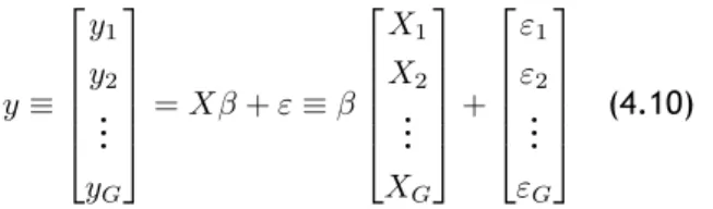
y≡       y1 y2 .. . yG      = Xβ + ε≡ β       X1 X2 .. . XG      +       ε1 ε2 .. . εG       (4.10)

We have G clusters, index by j, stacked into a vector y and a matrix X.β is a vector of unknown parameters. ε designate the OLS residuals for jth_{cluster that are robust to heteroskedasticity}

and cluster-correlations. The procedure for a wild cluster bootstrap a la Cameron et al. (2008) comes

y_ji= X_jiβ + f (ˆˆ εji)vj (4.11)

where j indexes clusters, i indexes observations, and the v derive from the Rademacher distri-bution. Davidson et al. (2007); Davidson and Flachaire (2008) recommend the usage of built-in Rademacher distribution weights vj{−1, 1} since they outperform Mammen (1993) two-point

distribution. The robustness check using wild-cluster bootstraped SE’s gave us the following output results. 4

Table 4.9: Estimation results with wild-cluster bootstraped SE’s

hhhhhhh_hhhhhhh

hh

Regressors

Dependent Variable

K_comp (1) L_comp (2) A_comp (3) BTC_comp (4)

csh_g -0.841*** -0.799** -0.263 0.321*** (0.224) (0.341) (0.458) (0.121) trade -0.45** -0.224 0.413 0.512*** (0.035) (0.169) (0.302) (0.05) hc 0.05 0.008 -0.224*** 0.116*** (0.042) (0.054) (0.068) (0.028) gwar -0.002 -0.004 0.024* -0.011 (0.01) (0.005) (0.013) (0.021) pd1 -0.001 -0.011** -0.002 0.017*** (0.007) (0.005) (0.007) (0.006) temp 0.001 0.004 -0.016*** 0.0017 (0.003) (0.005) (0.004) (0.002) ethnic -0.201 0.279** -0.182 0.124* (0.123) (0.127) (0.138) (0.086) Constant 0.765*** 0.396 1.127*** -0.337*** (0.147) (0.238) (0.208) (0.086)

Note: Regressors are defined in the first column of the Table. Dependent Variables are defined in the first row of the Table. Values in parentheses below the observed coefficients are the Cameron et al. (2008) wild bootstrapped multi-way clustered SE’s.Level of significance: *** for p-value > 0.01, ** for > 0.05, * for > 0.1. The number of replications used was 999. To reach the results we used the R package plm created by Graham et al. (2016) applying cluster.boot command.

Monte Carlos simulations done in Yu (2013) proved that Driscoll-Kraay’s SE’s perform very well

4_{The algorithm used to reach the results is on appendix R code A.1.}

Growth Accounting and Regressions