W O R K I N G PA P E R S E R I E S

W O R K I N G PA P E R S E R I E S

N O 9 7 1 / N O V E M B E R 2 0 0 8

INTERACTIONS BETWEEN

PRIVATE AND PUBLIC

SECTOR WAGES

W O R K I N G P A P E R S E R I E S

N O 9 71 / N O V E M B E R 2 0 0 8

In 2008 all ECB publications feature a motif taken from the 10 banknote.

INTERACTIONS BETWEEN PRIVATE

AND PUBLIC SECTOR WAGES

by António Afonso

and Pedro Gomes

This paper can be downloaded without charge from http://www.ecb.europa.eu or from the Social Science Research Network electronic library at http://ssrn.com/abstract_id=1302785.

1 We are grateful to Ad van Riet, Jürgen von Hagen, an anonymous referee, and participants at the 40th Money, Macro and Finance Research Group annual conference for helpful comments. The opinions expressed herein are those of the authors and do not necessarily reflect those of the European Central Bank or the Eurosystem. 2 European Central Bank, Directorate General Economics, Kaiserstrasse 29, D-60311 Frankfurt am Main, Germany. ISEG/TULisbon - Technical University of Lisbon, Department of Economics; UECE – Research Unit on

© European Central Bank, 2008

Address

Kaiserstrasse 29

60311 Frankfurt am Main, Germany

Postal address

Postfach 16 03 19

60066 Frankfurt am Main, Germany

Telephone

+49 69 1344 0

Website

http://www.ecb.europa.eu

Fax

+49 69 1344 6000

All rights reserved.

Any reproduction, publication and reprint in the form of a different publication, whether printed or produced electronically, in whole or in part, is permitted only with the explicit written authorisation of the ECB or the author(s).

The views expressed in this paper do not necessarily refl ect those of the European Central Bank.

Abstract 4

Non-technical summary 5

1 Introduction 7

2 Analytical framework 9

2.1 The model 9

2.2 Calibration and simulation 12

3 Empirical framework 15

3.1 Empirical specifi cation for private

sector wages 16

3.2 Empirical specifi cation for public

sector wages 18

3.3 Econometric issues 20

4 Estimation results and discussion 21

4.1 Data and stylised facts 21

4.2 Private wage determinants 22

4.3 Public wage determinants 24

4.4 Robustness, including further dynamics 26

5 Conclusion 27

References 27

Tables and fi gures 29

Appendices 37

European Central Bank Working Paper Series 53

Abstract

We analyse the interactions between public and private sector wages per employee in OECD countries. We motivate the analysis with a dynamic labour market equilibrium model with search and matching frictions to study the effects of public sector employment and wages on the labour market, particularly on private sector wages. Our empirical evidence shows that the growth of public sector wages and of public sector employment positively affects the growth of private sector wages. Moreover, total factor productivity, the unemployment rate, hours per worker, and inflation, are also important determinants of private sector wage growth. With respect to public sector wage growth, we find that, in addition to some market related variables, it is also influenced by fiscal conditions.

Keywords: public wages, private wages, employment.

Non-technical summary

The relevance of public wages for total public spending has gradually increased in

the past decades in several European countries. Apart from the importance that such

budgetary item has for the development of public finances and for attaining budgetary

objectives, public sector employment and wages play a key role on the labour market.

Therefore, the main objective of this paper is to understand the interactions between private

and public sector wages.

First, we motivate the analysis with a dynamic labour market equilibrium model with

search and matching frictions to study the effects of public sector employment and wages on

the labour market. As in other models that address this issue, we find that public sector wages

and employment have some impact on private sector wages. In essence, public sector wages

and employment impinge on private sector wage, via two channels. On one hand, they affect

the outside option of the unemployed, either by increasing the value of being employed in the

public sector (public sector wage) or by increasing the probability of being hired by the public

sector (public sector employment). Therefore, they put pressure on the wage bargaining. On

the other hand, both public wages and employment have to be financed by an increase in

taxes, which will reduce the overall gain from the match and increase the wage paid by the

firm. In the model, an increase of 1% in public sector wages induces an increase of 0.1% in

private sector wage. An increase in public employment of 1 percentage point of the labour

force increases private sector wages by 0.45%.

Second, we go on assessing the determinants of private sector wage growth. We

develop our analysis for the OECD and European Union countries for the period between

1970 and 1998/2006 (depending on data availability). We carefully discuss the econometric

An additional purpose of the paper is to analyse as well what are the main

determinants of public sector wages. For instance, public wages can also depend on the fiscal

position. Moreover, public wages might be used as an instrument in terms of income policies,

so they can depend on political factors such as the political alignment of the ruling party or

election cycles.

In a nutshell, we empirically find that a number of variables affect private sector

wage growth, for instance: changes in the unemployment rate (negative relationship),

inflation rate, total factor productivity growth and hours per worker. Moreover, public sector

wages and employment growth also affect private sector wage growth, which has important

policy implications. In addition, regarding the public sector wages, statistically significant

determinants are private sector wage growth, inflation, and changes in the unemployment rate

(positive relationship). Public sector wages also react positively to the budget balance and

negatively to government indebtedness, that is, to higher debt-to-GDP ratios.

1. Introduction

The relevance of public wages for total public spending has gradually increased in

the past decades in several European countries. Apart from the importance that such

budgetary item has for the development of public finances and for attaining budgetary

objectives,1 public sector employment and wages play a key role on the labour market.

Therefore, the main objective of this paper is to understand the interactions between private

and public sector wages.

First, we motivate the analysis with a dynamic labour market equilibrium model with

search and matching frictions to study the effects of public sector employment and wages on

the labour market. As in other models that address this issue,2 we find that public sector

wages and employment have some impact on private sector wages. In essence, public sector

wages and employment impinge on private sector wage, via two channels. On the one hand,

they affect the outside option of the unemployed, either by increasing the value of being

employed in the public sector (public sector wage) or by increasing the probability of being

hired by the public sector (public sector employment). Therefore, they put pressure on the

wage bargaining. On the other hand, both public wages and employment have to be financed

by an increase in taxes, which will reduce the overall gain from the match and increase the

wage paid by the firm. In the model, an increase of 1% in public sector wages induces an

increase of 0.1% in private sector wage. An increase in public employment of 1 percentage

point of the labour force increases private sector wages by 0.45%.

Second, we go on assessing the determinants of private sector wage growth. We

develop our analysis for the OECD and European Union countries for the period between

1

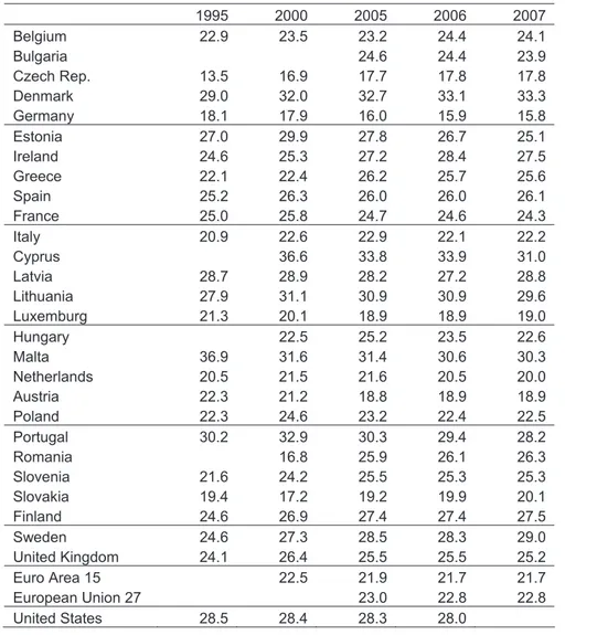
According to the European Commission, the average share of public wages (compensation of employees) in general government total spending was around 23 per cent in 2007 for the European Union, that is, around 11 percent of GDP. Interestingly, the public wages-to-total government spending ratio was 28 per cent in 2006 in the US. See the Appendix for some illustrative country data.

2

1970 and 1998/2006 (depending on data availability). We carefully discuss the econometric

issues involved, and how we deal with them, particularly the problem of endogeneity.

An additional purpose of the paper is to analyse as well, what are the main

determinants of public sector wages. Although there is evidence of some pro-cyclicality of

public wages (Lamo et al., 2007), their developments may be less aligned with those of

private wages. For instance, public wages can also depend on the fiscal position. In fact,

Poterba and Ruben (1995) and Gyourko and Tracy (1989) find that fiscal conditions affect

wages of public employees at a local level. Moreover, public wages might be used as an

instrument in terms of income policies, so they can depend on political factors such as the

political alignment of the ruling party or election cycles. For instance, Matschke (2003) finds

evidence of systematic public wage increases prior to a federal election in Germany.

In a nutshell, we empirically find that a number of variables affect private sector

wage growth, for instance: changes in the unemployment rate (negative relationship),

inflation rate, total factor productivity growth and hours per worker. Moreover, public sector

wages and employment growth also affect private sector wage growth, which has important

policy implications. In addition, regarding the public sector wages, statistically significant

determinants are private sector wage growth, inflation, and changes in the unemployment rate

(positive relationship). Public sector wages also react positively to the budget balance and

negatively to government indebtedness, that is, to higher debt-to-GDP ratios.

The paper is organised as follows. In section two we present an analytical

framework, relevant for the subsequent empirical analysis. In section three we present the

empirical setting and in section four we report and discuss the results. Section five

2. Analytical framework

2.1. The model

We set up a dynamic labour market equilibrium model, with public and private sectors

and search and matching frictions, along the lines of Pissarides (1988). The general setting

shares some features with Quadrini and Trigari (2007). Public variables are denoted with

superscript {g} while private sector variables are denoted by {p}. Households’ utility takes

the form

( ,_{t t}) _{t t}

u c g c Fg

, (1)

where c_t is private consumption and g_t is the flow of services derived from public

employment.

Part of the labour force is unemployed (u_t), while the remaining is either working in

the public sector (Lg_t ) or in the private sector (L_tp),

1 u_t Lg_t L_tp. (2)

Workers supply one unit of labour. If they are unemployed they search for jobs in

both public and private sectors. s_t gives the share of time devoted searching for a public

sector job. Firms post vacancies p t

v . The number of matches is determined by two matching

functions, one for each sector, and we allow for different matching coefficients Kp and

g

K _:

(1 )

((1 ) ) p p

p p p

t t t t

M m s u K v K , (3)

(1 )

( ) g g

g g g

t t t t

M m s u K v K . (4)

From the matching functions we can calculate the job finding rates (p_tgandp_tp) and

the probabilities of vacancies being filled (q_tpandq_tg):

, , ,

p g p g

p t g t p t g t

t p t g t t

t t t t

M M M M

q q p p

Government

The government hires workers to provide some public services, following a simple

linear functiong_t Lg_t . As in Quadrini and Trigari (2007), we assume that both public sector

employment and wages are set exogenously. It is not our purpose to identify the optimal level

of public employment and wages, but simply to understand the transmission mechanism of

public sector wages and employment shocks.

,

g g g g

t t

L L w w . (6)

Although the government targets the level of public employment, it has to post a

number of vacancies consistent with the following law of motion.

1 (1 )

g g g g g

t t t t

L O L q v . (7)

Every period a fraction Og

of public jobs are destroyed so the government posts the

number of public sector vacancies (v_tg) needed to maintain the level of employment, given

the current market conditions.

Finally, the government sets a labour income tax (W_t) necessary to finance the

government wage bill, the payment of unemployment benefits (z) and the cost of posting the

vacancies (cg),

(1p p ) g g g g

tL wt t t L wt t zut c vt

W W . (8)

Firms

Firms produce a good with a production function that only depends on labour.

(1 )

p

t t

Y AL D . (9)

The private sector labour follows the following law of motion

1 (1 )

p p p p p

t t t t

where Op

is the private sector job separation rate. At any point in time the level of

employment is predetermined and the firm can only control the number of vacancies it posts.

The objective of the firms is therefore to maximize the present discounted value of profits

subject to the law of motion of private employment,

(1 )

0

[ ]

k p p p p p

t t k t k t k t k

k

Max E E AL D L w c v

f

¦

where cpis the cost of posting a vacancy. The solution to this problem is given by the

following first order condition:

1 1

1

[ (1 ) (1 ) ]

p p

p p p

t t t

p p

t t

c c

E A L w

q q

D

E D O

. (12)

The optimality condition of the firm states that the expected cost of hiring a worker

must equal its expected return. The benefits of hiring an extra worker is the discounted value

of the expected difference between its marginal productivity and its wage and the

continuation value, knowing that with some probability Op the match can be destroyed.

Workers

The value to the household of each member depends on their current state: employed

in the public or in the private sector or unemployed. The value of being in each state is given

by the following expressions:

1 1

(1 ) [(1 ) ]

p p p p p

t t t t t t

W W w EE O W O U , (13)

1 1

(1 ) [(1 ) ]

g g g g g

t t t t t t

W W w EE O W O U , (14)

1 1 1

[ (1 ) ]

p p p g g p g

t t t t t t t t t

U z EE p W p W p p U . (15)

The value of unemployment depends on the level of unemployment benefits and on

the probabilities of finding a job in the two sectors. As the unemployed control the search

split their search optimally, by maximizing the value of unemployment. The optimal search of

public jobs is given implicitly by:

1 1 1 1

[ ] [ ]

1

g g g p p p

t t t t t t t t

t t

M E W U M E W U

s s

K K

. (16)

The optimal search of public sector jobs increases with the number of vacancies in the

public sector and the value of a public job, which depends positively on the public sector

wage and negatively on the separation probability. It is increasing in the importance of

unemployment and in the government matching function, and decreasing in the same

coefficient of the private sector matching function.

Wage bargaining

We consider that the private sector wage is the outcome of a Nash bargaining between

workers and firms. The solution is given by

(1b W)( _tpU_t) bJ_t, (17)

where b is the bargaining power of the worker and J_t is the value of an average job for the

firm, given by the following expression

1

(1 )

p p

t

t p t t

t

Y

J w J

L E O . (18)

2.2. Calibration and simulation

We calibrate the model to be, in general, representative on an OECD economy. Table

1 shows the baseline calibration. We consider public employment to be 15% of total labour

force, which, given an average unemployment rate of 8% is equivalent to, roughly, 16% of

wage premium is equal to 5%. This value is in line with several empirical estimates (see

Gregory and Borland, 1999, for an overview of the literature.

[Table 1]

The separation rate in the public sector is set to 3%, half the separation rate in the

private sector (6%). This follows Gomes (2008) that finds evidence of this for UK. We also

calibrate the two matching functions differently. As it is usual in the literature, we set Kp

equal to 0.5. In contrast, Kg is set equal to 0.3, which implies that vacancies are relatively

more important than the pool of unemployed in the public sector. We believe that this is a less

extreme assumption than the one used by Quadrini & Trigari (2007). They consider that the

unemployed queue for a public sector job which means that all public vacancies are filled.3

The other frictions parameters (ciand mi) are set equal in both sectors. Overall, the

calibration implies an unemployment rate of 8%, a job finding rate of 0.63 between the two

sectors, and a probability of filling a vacancy in the private sector of 0.5 and of 0.8 in the

public sector.

Following also the search and matching literature, the coefficient of the private wage

bargaining is set to 0.5. Finally, the unemployment benefit is set to 0.3, which implies a

replacement rate around 0.4, the discount factor is set to 0.99 and Įto 0.3.

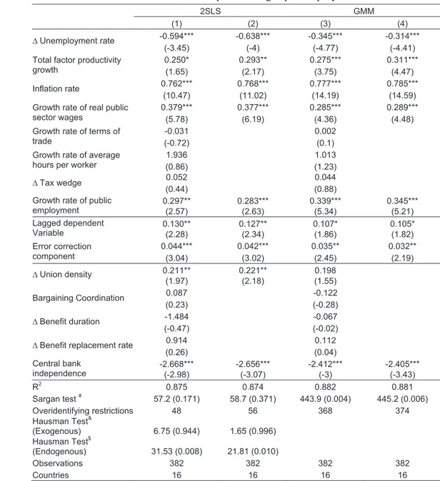
We can see in Figure 1 that the steady state level of private sector wages is positively

affected by the level of public sector wages and public sector employment.4

[Figure 1]

In essence, public sector wages and employment impinge on private sector wage, via

two channels. First, they affect the outside option of the unemployed, either by increasing the

3

In practice, the way that we calibrate the matching function is not important. The government decision variable is the level of public employment and vacancies adjust to guarantee that the new hires compensate the separations.

4

value of being employed in the public sector (public sector wage) or by increasing the

probability of being hired by the public sector (public sector employment). Therefore, they

put pressure on the wage bargaining. Second, both public wages and employment have to be

financed by an increase in taxes, which will reduce the overall gain from the match and

increase the wage paid by the firm. On average, an increase of 1% in public sector wages

induces an increase of 0.1% in private sector wage. An increase in public employment of 1%

of the labour force increases private sector wage by 0.45%.

Effects of temporary shocks in public sector employment and wages

We will now consider shocks to the level of public sector wages and employment of

the following type:

ln(w_tg) ln(wg)H H_t, ~_t AR(1), (19)

ln( g) ln( g) , ~ (1)

t t t

L L P P AR , (20)

with an autoregressive coefficient of the error of 0.8.

Figure 2 shows the response of public and private sector wages to a public sector

wage shock. We consider three cases with different levels of steady state public employment

(Lg 0.10,Lg 0.15 andLg 0.20). A temporary increase in public sector wage raises the

level of the private sector wage, but the magnitude of the response is, however, lower than if

the shock was permanent. A 1% increase in public sector wages increase private sector wages

by between 0.03% and 0.05%, depending on the size of the public sector. The bigger the size

of the government, the higher the effect of public sector wages on the labour market.

[Figure 2]

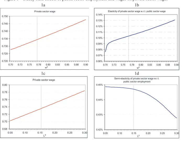
Figure 3 shows the response of private sector wages to a temporary increase of public

consider three alternative scenarios for the level of public sector wages (with low public

sector wages ( g/ p 1.00

w w ), the baseline case ( g / p 1.05

w w ) and one with higher public

sector wages (wg/wp 1.10). The impact on private sector wage occurs at the time of hiring,

and that is why the impact on the private sector wage is not very persistent. After two periods

it is close to zero. Nevertheless the contemporaneous effect is quite strong. Private sector

wages go up between 3% and 7%.

[Figure 3]

3. Empirical framework

In this section, we estimate the determinants of both private sector and public sector

wages. Our underlying idea is to estimate two different wage functions which link private and

public wages together, carefully addressing the problem of the endogeneity between the two.

Most papers that study the relation between the two wage variables usually focus on

wages per employee in levels (see, for instance, Nunziata, 2005, Jacobson and Ohlsson, 1994

and Friberg, 2007). However, we prefer to model growth rates, to assess the behaviour of the

two variables in the short-run. Since we have annual data, using growth rates eliminates the

low frequency movements but preserves the movements at business cycle frequency, which

we are more interested in uncovering (see Abraham and Haltiwanger, 1995).

In the long-run it is natural that the two variables are cointegrated with a slope

coefficient of one, otherwise, one would observe a constant divergence of the wages of the

two sectors. Notice that this does not exclude that there are differences in the levels of the

wages, but essentially that these differences do not have a trend. In fact, we observe and we

should expect either a public sector wage premium or a gap to exist, due to different skill

We study this issue in a panel framework for OECD and European Union country

groups, covering essentially the period between 1970 and 2007, depending also on data

availability.

3.1. Empirical specification for private sector wages

Our general baseline wage function for the developments in private sector salaries can

be given by

1 1

p p

it i p it it it p it it

w p

E

G

J

P

In (21) the index i (i=1,…,N) denotes the country, the index t (t=1,…,T) indicates the

period, Ei stands for the individual effects to be estimated for each country i, and it is assumed

that the disturbances P_it are independent across countries. wpit is the growth rate of the

nominal compensation per employee in the private sector.X_itpis a vector of macroeconomic

variables that might be endogenous to the private sector wage growth:

1 2 3 4 5 6 7 8

p

it it it it it it it it it

X

T

T

T

T

T

T

T

T

This vectorX_itpincludes the growth rate of real compensation per employee in the

public sector, wgit, the growth rate of the consumer price index, p, the growth rate of labour

productivity, l (or total factor productivity), the change in the unemployment rate, u, the

growth rate of the per worker average hours worked, h, tot denotes the growth rate of the

countries terms of trade, tw is the change in the tax wedge, while the growth rate of public

employment, eg, which can also positively impinge on the growth rate of private sector

wages, if higher labour demand in the public sector pressures private sector wages upward.

On the other hand, Z_itp is a vector of institutional exogenous variables

1 2 3 4 5

g

it it it it it it

which includes the change in union density, ud, an index of bargaining coordination, bc,the

change in benefit duration, bd, the change in the benefit replacement ratio, brr and previous

work by Nunziata (2005) concluded that these institutional variables were important

determinants of the level of wages. While union density should contribute to increase wages,

the benefit replacement rate and duration all affect the outside option of the worker, and

therefore may also influence their wage. Additionally if the bargaining process is centrally

coordinated it is likely to restrain private sector wage growth. We also include an index of

central bank independence, cbi, to capture potential inflation expectations.

Finally,E_it1 in (21) is defined as the percentage difference between public and

private sector wages – the public wage premium or gap:

1 ln( 1/ 1) 100

it t t

E Wg Wp u , (24)

where Wg and Wp are respectively the nominal public and private wage levels per employee.

This term can be interpreted as an error correction mechanism. In this sense, if private and

public sector wages start diverging,J_p, in equation (21), measures whether part of the

re-balancing is done via the private sector wages.

There are two ways via which public sector wages can affect private sector wages.

There is the direct effect,T₁, and there is the indirect effect through the error correction

mechanism of magnitudeJ_p. If the ratio of public-to-private wages increases, private sector

wages may raise in order to correct the wage differential downwards. This can be seen both as

a demonstration effect stemming from the public sector, followed by the private sector, and as

well as a catching up effect in salaries demanded (implemented) by (in) the private sector.

Therefore, J_p is expected to be positive.

Additionally, in a specification such as (21)-(22), and according to the estimated value

imply a pro-cyclical behaviour of private wages towards unemployment, and a positive T₆

implies a counter-cyclical response of wages to unemployment. While the idea of wage

counter-cyclicality was already put forward notably by Keynes (1939), empirical results

actually produce evidence of both cyclical and counter cyclical private sector behaviour.

Abraham and Haltiwanger (1995) offer several arguments for the possibility of both

outcomes.

This specification for the private sector wage growth is inspired by the theoretical

model, but with a few differences. First, given that there is long-run growth, which was

absent from the model, we estimate the equation in growth rates and include the error

correction term. Second, we include several variables that were absent from the model.

3.2. Empirical specification for public sector wages

We also estimate an equation for the public sector wage growth. This equation has

somewhat less motivation from the theoretical part, given that we consider public sector

wages as exogenous. The baseline wage function for the developments of public sector

salaries can be assessed with the following specification

1 1

g g

it i g it it it g it it it it

w g D G w g X Z J E F P P , (25)

with

1 2 3 4 5 6

g

it it it it it it it

X

G

G

G

G

G

G

1 2 3 4

g

it it it it it

Z

K

K

K

K

1 2

it it it

F ZBudBal Z Debt , (28)

1 2

it it it

P OElection O Left . (29)

We consider that the government wage can respond to the same variables as the

growth rate of public employment. Indeed, the hours worked in the public sector are more

standardized than in the private sector, and the variable average hours per worker is likely to

be also more relevant for the private sector. Additionally, F_it includes fiscal variables such as

the general government budget balance as a percentage of GDP and the general government

debt-to-GDP ratio. P_it contains the political variables, which consist of the percentage of

votes for left wing parties and a dummy variable for parliamentary election years. While the

variables in F_it are endogenous, we consider the variables inP_it as exogenous. Di stands for

the individual effects to be estimated for each country i.

Similarly to the specification for the private sector wages, J_gnow measures to what

extent public wages correct the imbalances of the long-term relation between public sector

and private sector wages. In this case, increases in the public wages-to-private wages ratio

can produce afterwards a reduction in public sector wages, implying an expected negative

value forJ_g.

While one would expect that recent fiscal developments may impinge on the

development of the public sector wages per employee, this hypothesis is seen as less relevant

for the development of private sector wages. On the other hand, if one expects the

unemployment rate to impinge negatively on the development of private sector wages, this

effect may essentially be more mitigated or even absent in the case of public sector wages,

given the higher rigidity of the labour force in the government sector (and a possible higher

degree of unionisation). Finally, one should be aware that this aggregate analysis does not

directly take into account such issues as labour flows between the two sectors or within the

private sector, while different wage scales also co-exist inside the private sector, with

3.3. Econometric issues

There are two main econometric issues when estimating the wage functions (21) and

(25). The first issue is the presence of endogenous variables, particularly the simultaneous

determination of public and private sector wage growth. To deal with this, we estimate each

equation separately and instrument all the endogenous variables by the remaining

pre-determined variables and three lags of all variables. We compute the Sargan over-identifying

test to access the validity of the instruments. As we are using the lagged variables as

instruments, essentially what we are doing is predicting the value of the regressors based on

past information, so the interpretation of the coefficients should be, for instance, the effect of

expected public sector wage growth on the growth rate of private sector wages.

Although our distinction between endogenous and exogenous variables might seem

arbitrary, we also run a Hausman test in some of the estimations to examine the exogeneity of

each block of variables.

The second issue is that, as we allow for a country specific error and include a lagged

dependent variable, our specification has a correlation between a regressor and the error term.

Although we also use the Arellano and Bond GMM estimator, our preferred methodology is a

simple panel 2SLS estimation. First, the Arellano and Bond methodology implies estimating

the equation in first differences (of growth rates) which inserts a lot of noise in the estimates.

Furthermore, as Nickell et al. (2005) point out, the bias created by the presence of a lagged

dependent variable in panel data, tends to zero if we have a long time series component. As

we have close to 30 average time observations per country, we proceed with the estimation

with a panel 2SLS. We also include country fixed effects, and we estimate the equations for

4. Estimation results and discussion

4.1. Data and stylised facts

Our main data source is the OECD Economic Outlook database, essentially for the

employment and wages data, the European Commission database AMECO and the Labour

Market Institutions Database used in Nickell et al. (2005) and expanded by Baker et al.

(2003).5 Private sector wages are defined as total compensation of employees minus

compensation of government employees. Private sector wages per employee are defined as

private compensation of employees divided by private sector employees (total employment

minus government employees minus self-employed persons).6 We compute the real wage per

employee using the consumption price deflator. Although we think it is useful to use

aggregate data to study the issues at hand, we should be aware of its limitations. The main

problem is that it ignores the composition of public and private employment, in particular

with respect to the skill level of the employment.

A cursory look at the main data series provides a first useful insight regarding past

trends. The charts that we report in Appendix 3, regarding salaries and employment shares,

show that while the share of government employment in total employment increased for most

countries in the 1980s, there was an even more generalised decline after the beginning of the

1990s.

Regarding real wage per employee an upward trend can be observed for most

countries, both for private and for government salaries. Nevertheless, a decline in real private

wages per employee was visible for Italy and Spain since the middle of the 1990s, which also

needs to be seen against the increase in female labour participation. Interestingly, real public

wages per employee were rather stable for Japan, Germany and Austria since the beginning of

5

Given data availability, the countries used in the empirical analysis are Australia, Belgium, Canada, Denmark, Finland, France, Germany, Ireland, Italy, Japan, Netherlands, Norway, Spain, Sweden, United Kingdom and United States. See Appendix 1 for further details and sources.

6

the 1990s. The mean and the volatility of private wage growth, reported in Appendix 2, were

rather similar to the ones of public wage growth

A further stylised fact is given by the development of the ratio of public-to-private

wages per employee, which broadly followed an upward path since the beginning of the

1990s for most European countries. However, such ratio was more stable in the Netherlands,

and to some extent in Sweden, while developments were more mixed for the US and Norway.

On the other hand, the ratio of public-to-private wages per employee decreased in Canada and

in Australia.

4.2. Private wage determinants

Table 2 reports the results for the growth rate of the nominal private sector wages per

employee, for the OECD countries. The estimated coefficients are quite similar across the

estimation method. In the case of nominal private sector wages we should focus more on the

results from 2SLS as the GMM estimators does not pass the Sargan test.

One can observe that both the direct effect and the indirect effect – via the ratio

between public wages and private wages – of public sector wages are statistically significant

and positive, as expected. A 1% increase in real public sector wage growth increases private

sector nominal wage growth by 0.3%.

[Table 2]

The growth rate of public employment also has a positive and significant effect on the

growth rate of nominal private sector wages. A 1 percent in public sector employment

increases private sector wage growth by close to 0.3%.

The change in the unemployment rate exerts a negative effect on private sector wage

unemployment rate reduces the growth rate of nominal private sector wages by around

0.3-0.6 percentage points. On the other hand, private sector wages increase with total factor

productivity growth (labour productivity was not statistically significant). Moreover, an

increase in the inflation rate of 1 percentage point translates into an increase in the growth

rate of nominal private sector wages of around 0.8 percentage points. Some wage stickiness is

captured by the statistically significant lagged dependent variable. There are no statistically

significant effects reported for the terms of trade, for the hours worked per worker or for the

tax wedge.

Regarding the set of pre-determined explanatory variables (in vector Z), it is

interesting to see that the growth rate of nominal private sector wages is positively affected by

the degree of union density, implying that an increase in unionisation may translate into

higher private wage growth. Higher central bank independence has an opposite effect,

therefore contributing to reduce the growth rate of nominal private sector wages. Benefit

duration, and the benefit replacement rate do not statistically affect the growth rate of nominal

private sector wages.

To further assess our results, we also report the estimations for the specification

regarding the growth rate of real private sector wages per employee in Table 3. Both

estimations pass the Sargan test, although the GMM estimations have a slightly higher

R-square.

[Table 3]

We can see that in this case, the lagged value of the dependent variable is still

statistically significant, while the growth rate of average hours per worker now contributes to

increase the growth rate of real private sector wage per employee. Another difference that

wages per employee.7 The statistical significance and the estimated coefficients of the

remaining explanatory variables are rather similar to the specification for the growth rate of

nominal private sector wages, notably the indirect effect of public wages via the error

correction component.

In the estimations, for both nominal and real private sector wage growth, the Hausman

test clearly supports that the institutional variables block is exogenous and that the variables

in the macroeconomic block are endogenous.

4.3. Public wage determinants

We now turn to the analysis of the determinants of public sector wages, and the

corresponding estimation results for nominal wages are presented in Table 4. All the

estimations pass the Sargan test.

[Table 4]

The lagged dependent variable is statistically significant, denoting some degree of

public sector wage stickiness. The growth rate of nominal public sector wages per employee

also reacts positively to real private sector wages, with a coefficient between 0.5 and 0.9. It

also responds negatively to an increase in the ratio between public and private sector wages.

Therefore, this correction mechanism adjusts public wages downward when the differential

vis-à-vis private wages rises. Note that the absolute value of the coefficient is roughly three

times higher than the one from the similar error correction component’s coefficient estimated

in the private sector model. This means that three quarters of the adjustment is done via

public sector wages.

An increase in the inflation rate also increases the growth rate of nominal public

sector wages and the magnitude of this effect is around 0.6 percentage points. Total factor

productivity is negatively related to the growth rate of nominal public sector wages, and this

can be explained by the fact that the productivity measure pertains essentially to the private

sector. The terms of trade do not statistically affect the growth rate of nominal public sector

wages.

Regarding the two explanatory fiscal variables, improvements in the budget balance

increase the growth rate of nominal public sector wages, while a higher government

debt-to-GDP ratio reduces it. An increase in the budget balance ratio of 1 percentage point translates

into an increase of the growth rate of nominal public sector wages of around 0.1 percentage

points. Interestingly, in the GMM estimations, higher government indebtedness is related

with decreases in the growth rate of nominal public sector wages. In terms of the

pre-determined exogenous variables it is not possible to observe any statistically significant

negative effect associated either with bargaining coordination or with benefits duration, and

the same is true for the political dummy variables.

When using the growth rate of real public sector wages per employee as dependent

variable (Table 5), the inflation rate has a negative impact. This suggests that, unlike the

private sector, the public sector wages are more able to contain the repercussion of expected

inflation on the public sector wage growth. On the other hand, real public wages react

positively to increases in the unemployment rate. The effects of the other explanatory

variables still hold, and improvements in the budget balance notably contribute to increase

real public wages per employee.

We also considered only the subset of European Union and euro area countries in our

empirical analysis (see Appendix 2). The results are rather similar to the ones for the OECD

country sample. Nevertheless, the magnitude of the effect of the budget balance on public

wages is now slightly higher.

4.4. Robustness, including further dynamics

In our baseline estimations, the only dynamic element is the inclusion of the lagged

dependent variable. Even if that coefficient is small one could argue that there might be direct

effects of past explanatory variables on the regressors. Therefore, we included in the

regressions one lag of all explanatory variables. Most lags of the variables are not significant.

As we are interested on the overall effect of a variable on the wage growth, in Table 6 we

only report the sum of the two coefficients (contemporaneous and lagged) and the p-value of

the test that the sum of the two coefficients is different from zero. Basically, the main results

from the baseline specification remain: notably, there is a spillover of both private and public

wages, through the direct effect and via the error correction mechanism, as well as the effect

of public employment on private wages.

[Table 6]

In addition, it seems that the inclusion of lags do not carry much explanatory power in

this case. Indeed, the R-square changes very little, and the test that all coefficients of the

lagged explanatory variables are jointly equal to zero is accepted for the 2SLS case of public

sector wages. Consequently, there isn’t much gain from the inclusion of the above mentioned

lags, which just increases the standard deviations and reduces the significance of some

5. Conclusion

The purpose of this paper was to uncover the determinants of public and private sector

wage growth. We also find that a number of variables affect private sector wage growth, for

instance: unemployment rate (negative relationship), inflation rate, total factor productivity,

and hours per worker. More important, public sector wages and employment also affect

private sector wage growth. In terms of magnitude, the estimated values are higher than the

values suggested by the model. The empirical estimates show a contemporaneous effect of

around 0.3% private sector wages with respect to public sector wages. Higher public sector

wages might translate into higher demand, increasing the pressure on the private sector labour

market. Similarly, public sector wage growth may also carry a signal to the private sector on

what the government expects for inflation.

This finding has important policy implications. It gives strength to the “wage twist”

policy discussed by Pedersen et al. (1990). Therefore, the governments could use their role as

an employer to reduce relative public sector wages. This policy, besides reducing the tax

burden necessary to finance government spending, would have a downward impact on

private sector wages and, most likely, on inflation and unemployment.

Regarding the public sector wages, statistically significant determinants are private

sector wages, inflation, and the unemployment rate (positive relationship). Moreover, public

sector wages react positively to the budget balance and negatively to government

indebtedness. Political variables, however, do not seem to play an important role

References

Abraham, K. and Haltiwanger, J. (1995). “Real Wages and the Business Cycle”, Journal of

Algan, Y.; Cahuc, P. and Zylberberg, A. (2002). "Public employment and labour market

performance", Economic Policy, 17 (34), 7-66.

Ardagna, S. (2007). “Fiscal policy in unionized labor markets”, Journal of Economic

Dynamics and Control, 21 (5), 1498-1534.

Baker, D.; Glyn, A.; Howell, D. and Schmitt, J. (2003). “Labor Market Institutions and

Unemployment: A Critical Assessment of the Cross-Country Evidence”, Economics Series

Working Papers 168, University of Oxford, Department of Economics.

Forni, L. and Giordano, R. (2003). “Employment in the public sector”, CESifo WP 1085.

Friberg, K. (2007). “Intersectoral wage linkages: the case of Sweden”, Empirical Economics,

32 (1), 161-184.

Gomes, P. (2008) “Labour market flows: facts from UK”, Bank of England Working Papers,

forthcoming.

Gregory, R. and Borland, J. (1999). “Recent developments in public sector labor markets”, in

Ashenfelter, O. and Card, D. (eds), Handbook of Labor Economics, vol III. Amsterdam,

Elsevier Science Publishers.

Gyourko, J. and Tracy, J. (1989). “The Importance of Local Fiscal Conditions in Analyzing

Local Labor Markets”, Journal of Political Economy, 97 (5), 1208-31.

Holmlund, B. and Linden, J. (1993). “Job matching, temporary public employment, and

equilibrium unemployment”, Journal of Public Economics, Elsevier, 51 (3), 329-343.

Jacobson, T. and Ohlsson, H. (1994). “Long-Run Relations between Private and Public Sector

Wages in Sweden”, Empirical Economics, 19 (3), 343-60.

Keynes, J. (1939). “Relative Movements of Real Wages and Output”, Economic Journal,

(193), 34-51.

Lamo, A.; Pérez, J. and Schuknecht, L. (2007). “The cyclicality of consumption, wages and

Matschke, X. (2003). “Are There Election Cycles in Wage Agreements? An Analysis of

German Public Employees”, Public Choice, 114 (1-2), 103-35.

Nickell, S.; Nunziata, L. and Ochel, W. (2005). "Unemployment in the OECD since the

1960s. What Do We Know?" Economic Journal, 115, 1-27.

Nunziata, L. (2005). "Institutions and Wage Determination: a Multi-country Approach",

Oxford Bulletin of Economics and Statistics, 67 (4), 435-466.

Pedersen, P.; Schmidt-Sorensen, J.; Smith, N. and Westergard-Nielsen, N. (1990). “Wage

differentials between the public and private sectors”, Journal of Public Economics, 41 (1),

125-145.

Pissarides, C. (1988). “The search equilibrium approach to fluctuations in employment”,

American Economic Review, 78 (2), 363-68.

Poterba, J. and Ruben, K. (1995). “The Effect of Property-Tax Limits on Wages and

Employment in the Local Public Sector”, American Economic Review, 85 (2), 384-89.

Quadrini, V. and Trigari, A. (2007). “Public employment and the business cycle”,

Scandinavian Journal of Economics, 109 (4), 723-742.

Tables and Figures

Table 1 – Baseline calibration

1

A D 0.3 b 0.5 E 0.99 z 0.3

0.6

p

m cp 0.17 Kp 0.5 Op 0.06 wg 0.77

0.6

g

m cg 0.17 Kg 0.3 Og 0.03 Lg 0.15

0.08

u p _0.52

q pp 0.57 s 0.19

/ 1.05

g p

Table 2 – Nominal private wages per employee

2SLS GMM

(1) (2) (3) (4)

-0.594*** -0.638*** -0.345*** -0.314***

¨Unemployment rate

(-3.45) (-4) (-4.77) (-4.41)

0.250* 0.293** 0.275*** 0.311***

Total factor productivity

growth _{(1.65) (2.17) (3.75) (4.47)}

0.762*** 0.768*** 0.777*** 0.785*** Inflation rate

(10.47) (11.02) (14.19) (14.59) 0.379*** 0.377*** 0.285*** 0.289*** Growth rate of real public

sector wages _{(5.78) (6.19) (4.36) (4.48)}

-0.031 0.002 Growth rate of terms of

trade _{(-0.72) (0.1)}

1.936 1.013 Growth rate of average

hours per worker (0.86) (1.23)

0.052 0.044

¨Tax wedge

(0.44) (0.88) 0.297** 0.283*** 0.339*** 0.345*** Growth rate of public

employment (2.57) (2.63) (5.34) (5.21)

0.130** 0.127** 0.107* 0.105* Lagged dependent

Variable (2.28) (2.34) (1.86) (1.82)

0.044*** 0.042*** 0.035** 0.032** Error correction

component (3.04) (3.02) (2.45) (2.19)

0.211** 0.221** 0.198

¨Union density

(1.97) (2.18) (1.55)

0.087 -0.122

Bargaining Coordination

(0.23) (-0.28)

-1.484 -0.067

¨Benefit duration

(-0.47) (-0.02) 0.914 0.112

¨Benefit replacement rate

(0.26) (0.04) -2.668*** -2.656*** -2.412*** -2.405*** Central bank

independence (-2.98) (-3.07) (-3) (-3.43)

R2

0.875 0.874 0.882 0.881

Sargan test # 57.2 (0.171) 58.7 (0.371) 443.9 (0.004) 445.2 (0.006) Overidentifying restrictions 48 56 368 374 Hausman Test&

(Exogenous) 6.75 (0.944) 1.65 (0.996) Hausman Test$

(Endogenous) 31.53 (0.008) 21.81 (0.010)

Observations 382 382 382 382

Countries 16 16 16 16

Notes: The following variables are considered endogenous: change in unemployment rate, growth rate of total factor productivity, inflation rate, growth rate of real per worker public sector wages, growth rate of terms of trade, growth rate of hours per worker, change in tax wedge and the growth rate of public employment. These endogenous variables are instrumented by the remaining pre-determined variables and three lags of all explanatory variables. The t statistics are in parentheses. For the 2SLS estimation, the conventional standard errors were used. For the Arellano and Bond GMM estimator robust standard errors were used.. *, **, *** - statistically significant at the 10, 5, and 1 percent.. _{White diagonal standard errors & covariance (d.f. corrected).} #

The null hypothesis of the Sargan overidentification test is that the instruments are uncorrelated with the error term and that the excluded instruments are correctly excluded from the estimated equation. Under the null, the test statistic is distributed as chi-squared in the number of overidentifying restrictions. The p-value is in brackets. & The null hypothesis is that the block of institutional variables is exogenous. Under the null, the estimator used is efficient but is is inconsistent under the alternative hypothesis. The consistent estimator would be to consider all variables as endogenous and instrument them with lags. The p-value is in brackets. $ The null hypothesis is that the block of macroeconomic variables is exogenous. Under the null, the most efficient estimator is fixed effects estimation taking all variables as exogenous. Under the alternative hypothesis the estimates are consistent estimates. The p-value is in brackets.

Table 3 – Real private wages per employee

2SLS GMM

(1) (2) (3) (4)

-0.430** -0.344** -0.228** -0.233***

¨Unemployment rate

(-2.46) (-2.48) (-2.48) (-2.61)

0.15 0.251*** 0.263***

Total factor productivity

growth _{(1.02) (3.51) (4.04)}

0.013 -0.034

Inflation rate

(0.3) (-1.53)

0.357*** 0.346*** 0.308*** 0.321*** Growth rate of real public

sector wages _{(5.43) (5.78) (4.96) (5.17)}

0.007 0.025 Growth rate of terms of

trade _{(0.14) (1.13)}

3.939* 4.884*** 1.739** 1.978**

Growth rate of average

hours per worker (1.72) (2.6) (2.19) (2.28)

-0.013 0.036

¨Tax wedge

(-0.11) (0.65) 0.249** 0.257*** 0.334*** 0.308*** Growth rate of public

employment (2.2) (3.29) (5.83) (5.3)

0.130** 0.137*** 0.163*** 0.152*** Lagged dependent

Variable (2.34) (2.82) (3.14) (3.31)

0.042*** 0.044*** 0.030* 0.031** Error correction

component (2.95) (3.39) (1.91) (2.07)

0.170 0.174* 0.147

¨Union density

(1.62) (1.74) (1.27)

-0.084 -0.217 Bargaining Coordination

(-0.23) (-0.46) -1.088 -0.897

¨Benefit duration

(-0.35) (-0.27)

1.384 -0.173

¨Benefit replacement rate

(0.4) (-0.06)

-2.378*** -2.550*** -2.058*** -1.937*** Central bank

independence (-2.72) (-3.07) (-2.86) (-2.71)

R2

0.355 0.338 0.381 0.368

Sargan test # 51.9 (0.290) 52.2 (0.543) 387.2 (0.223) 401.1 (0.161) Overidentifying restrictions 47 56 367 374 Hausman Test&

(Exogenous) 5.65 (0.975) 0.38 (1.000) Hausman Test$

(Endogenous) 22.27 (0.101) 17.50 (0.025)

Observations 382 382 382 382

Countries 16 16 16 16

Notes: The following variables are considered endogenous: change in unemployment rate, growth rate of total factor productivity, inflation rate, growth rate of real per worker public sector wages, growth rate of terms of trade, growth rate of hours per worker, change in tax wedge and the growth rate of public employment. These endogenous variables are instrumented by the remaining pre-determined variables and three lags of all explanatory variables. The t statistics are in parentheses. For the 2SLS estimation, the conventional standard errors were used. For the Arellano and Bond GMM estimator robust standard errors were used.. *, **, *** - statistically significant at the 10, 5, and 1 percent.. _{White diagonal standard errors & covariance (d.f. corrected).} #

The null hypothesis of the Sargan overidentification test is that the instruments are uncorrelated with the error term and that the excluded instruments are correctly excluded from the estimated equation. Under the null, the test statistic is distributed as chi-squared in the number of overidentifying restrictions. The p-value is in brackets. . & The null hypothesis is that the block of institutional variables is exogenous. Under the null, the estimator used is efficient but it is inconsistent under the alternative hypothesis. The consistent estimator would be to consider all variables as endogenous and instrument them with lags. The p-value is in brackets. $ The null hypothesis is that the block of macroeconomic variables is exogenous. Under the null, the most efficient estimator is fixed effects estimation taking all variables as exogenous. Under the alternative hypothesis the estimates are consistent estimates. The p-value is in brackets.

Table 4 – Nominal public wages per employee

2SLS GMM

(1) (2) (3) (4)

0.485** 0.472** 0.009

¨Unemployment rate

(1.96) (2.13) (0.06) -0.394** -0.388** -0.124 Total factor productivity

growth (-2.02) (-2.04) (-1.09)

0.569*** 0.570*** 0.574*** 0.576*** Inflation rate

(7.43) (8.03) (12.51) (11.46)

0.826*** 0.880*** 0.480*** 0.475*** Growth rate of real private

sector wages _{(5.64) (6.64) (7.12) (6.85)}

-0.055 0.011 Growth rate of terms of

trade (-0.88) (0.51)

-0.093 -0.048

¨Tax wedge

(-0.53) (-0.6) 0.135** 0.123* 0.123* 0.125** Budget Balance

(2.06) (1.95) (1.7) (2.01)

-0.016 -0.021 -0.029* -0.030**

Government debt

(-1.09) (-1.49) (-1.76) (-2.02) 0.214*** 0.222*** 0.250*** 0.253*** Lagged dependent

Variable (4.28) (4.57) (3.52) (3.68)

-0.108*** -0.114*** -0.106*** -0.113*** Error correction

component (-5.47) (-5.95) (-6.82) (-6.56)

0.077 0.239 0.201

¨Union density

(0.49) (1.57) (1.29)

-0.331 -0.447 0.000

Bargaining Coordination

(-0.65) (-0.69) -5.211 -4.633

¨Benefit duration

(-1.12) (-1.39) 0.964 2.346

¨Benefit replacement rate

(0.2) (0.53)

-0.141 -0.139 Election year

(-0.47) (-0.49) 0.049 0.041 % Left wing votes

(1.17) (0.84)

R2 0.778 0.773 0.800 0.796

Sargan test p-value #

52.02 (0.285) 54.7 (0.487) 393.5 (0.155) 406.6 (0.126) Overidentifying restrictions 47 55 366 375 Hausman Test&

(Exogenous) 5.13 (0.995) - Hausman Test$

(Endogenous) 42.62 (0.000) 87.75 (0.000)

Observations 382 382 382 382

Countries 16 16 16 16

Notes: The following variables are considered endogenous: change in unemployment rate, growth rate of total factor productivity, inflation rate, growth rate of real per worker private sector wages, growth rate of terms of trade, growth rate of hours per worker, budget balance, government debt and tax wedge. These endogenous variables are instrumented by the remaining pre-determined variables and three lags of all explanatory variables. The t statistics are in parentheses. For the 2SLS estimation, the conventional standard errors were used. For the Arellano and Bond GMM estimator robust standard errors were used.. *, **, *** - statistically significant at the 10, 5, and 1 percent.. _White diagonal standard errors & covariance (d.f. corrected). # The null hypothesis of the Sargan overidentification test is that the instruments are uncorrelated with the error term and that the excluded instruments are correctly excluded from the estimated equation. Under the null, the test statistic is distributed as chi-squared in the number of overidentifying restrictions. The p-value is in brackets. . & The null hypothesis is that the block of institutional variables is exogenous. Under the null, the estimator used is efficient but it is inconsistent under the alternative hypothesis. The consistent estimator would be to consider all variables as endogenous and instrument them with lags. The p-value is in brackets. $ The null hypothesis is that the block of macroeconomic variables is exogenous. Under the null, the most efficient estimator is fixed effects estimation taking all variables as exogenous. Under the alternative hypothesis the estimates are consistent estimates. The p-value is in brackets.

Table 5 – Real public wages per employee

2SLS GMM

(1) (2) (3) (4)

0.658*** 0.655*** 0.166 0.202*

¨Unemployment rate

(2.74) (3.05) (1.51) (1.76) -0.377* -0.361* -0.113

Total factor productivity

growth (-1.94) (-1.92) (-1.07)

-0.104 -0.130** -0.126** -0.119*** Inflation rate

(-1.6) (-2.26) (-2.57) (-2.66)

0.765*** 0.793*** 0.514*** 0.515*** Growth rate of real private

sector wages _{(5.26) (6.03) (8.36) (8.25)}

0.015 0.048 0.052

Growth rate of terms of

trade (0.23) (1.64) (1.63)

-0.175 -0.069

¨Tax wedge

(-0.96) (-0.94) 0.139** 0.136** 0.104 0.102 Budget Balance

(2.14) (2.22) (1.45) (1.63)

-0.012 -0.018 -0.029* -0.030**

Government debt

(-0.79) (-1.3) (-1.93) (-2.12) 0.209*** 0.211*** 0.241*** 0.248*** Lagged dependent

Variable (4.29) (4.65) (4.03) (3.91)

-0.111*** -0.119*** -0.115*** -0.119*** Error correction

component (-5.68) (-6.35) (-7.33) (-6.26)

0.019 0.18

¨Union density

(0.12) (1.06) -0.614 -0.572 Bargaining Coordination

(-1.22) (-1)

-4.316 -4.889** -5.217**

¨Benefit duration

(-0.93) (-2.13) (-2.25)

0.853 1.708

¨Benefit replacement rate

(0.17) (0.44) -0.327 -0.255 Election year

(-1.1) (-0.87)

0.034 0.025 % Left wing votes

(0.81) (0.55)

R2 0.388 0.381 0.427 0.415

Sargan test p-value #

49.8 (0.325) 54.1 (0.471) 372.6 (0.395) 377.1 (0.431) Overidentifying restrictions 46 56 366 373 Hausman Test&

(Exogenous) 4.57 (0.998) - Hausman Test$

(Endogenous) 50.60 (0.000) 44.2 (0.000)

Observations 382 382 382 382

Countries 16 16 16 16

Notes: The following variables are considered endogenous: unemployment rate, growth rate of total factor productivity, inflation rate, growth rate of real per worker private sector wages, terms of trade, hours per worker, budget balance, government debt and tax wedge. These endogenous variables are instrumented by the remaining pre-determined variables and three lags of all explanatory variables. The t statistics are in parentheses. For the 2SLS estimation, the conventional standard errors were used. For the Arellano and Bond GMM estimator robust standard errors were used. *, **, *** - statistically significant at the 10, 5, and 1 percent.. _{White diagonal standard errors & covariance (d.f.} corrected). # The null hypothesis of the Sargan overidentification test is that the instruments are uncorrelated with the error term and that the excluded instruments are correctly excluded from the estimated equation. Under the null, the test statistic is distributed as chi-squared in the number of overidentifying restrictions. The p-value is in brackets. & The null hypothesis is that the block of institutional variables is exogenous. Under the null, the estimator used is efficient but it is inconsistent under the alternative hypothesis. The consistent estimator would be to consider all variables as endogenous and instrument them with lags. The p-value is in brackets. $ The null hypothesis is that the block of macroeconomic variables is exogenous. Under the null, the most efficient estimator is fixed effects estimation taking all variables as exogenous. Under the alternative hypothesis the estimates are consistent estimates. The p-value is in brackets.