www.rbgf.org.br
DOI: 10.22564/rbgf.v37i4.2027
COMPARING TWO MULTIVARIATE GEOSTATISTICS TOOLS
FOR PORE PRESSURE PREDICTIVE MODELLING
Flávia Braz Ponte
1, Francisco Fábio de Araújo Ponte
2, Adalberto Silva
2and Alberto Garcia Figueiredo Jr
2ABSTRACT.Pore pressure prediction has been an increasing concern during well designing due to the numerous accidents recorded because of mistaken estimations of high pressure fields. This paper depicts a predictive modelling of pore pressure using multivariate geostatistics tools called LVM and collocated cokriging. The resulting maps of LVM and collocated cokriging were compared. Geostatistics were used to estimate pore pressure distribution in unsampled places considering the two different scales and spatial variation from well measurements (pore pressure) and 3D seismic velocity data. When pore pressure gradients recorded in the wells have been defined and the seismic interval velocity analyzed, pore pressure estimation can be done by using the geostatistics approaches. This is a method for estimating the geopressure field distribution at basin or reservoir level that offers the advantage of the possibility of extracting pore pressure information at any place within the modeled area.
Keywords: geostatistics approaches, LVM, collocated cokriging, high pressure fields.
RESUMO.Devido aos numerosos acidentes registrados por estimativas equivocadas de campos de alta pressão, a preocupação com a previsão de pressão de poros tem aumentado durante projetos de poços. Este artigo descreve uma modelagem para previsão de pressão de poros usando duas ferramentas da geoestatística multivariada, a LVM e a cokrigagem colocada. Neste estudo, essas duas metodologias foram comparadas. A geoestatística foi utilizada para estimar a distribuição de pressão de poros em locais não amostrados, permitindo a integração dos dados das duas variáveis, velocidade sísmica e dados de poço, em diferentes escalas e variação espacial. Quando os gradientes de pressão de poros, registrados em poços, são definidos e a velocidade intervalar da sísmica é analisada, existindo correlação entre eles, a previsão de pressão de poros pode ser feita utilizando a abordagem geoestatística. A vantagem de uma modelagem geoestatística 3D de gradiente pressão de poros é a possibilidade de extração de informação de pressão em qualquer local dentro da área modelada.
Palavras-chave: abordagem geoestatística, LVM, cokrigagem colocada, campos de alta pressão.
Corresponding author: Flávia Braz Ponte
1ENAUTA – Av. Almirante Barroso, 52, sala 1301, Centro, 20031-918, Rio de Janeiro, RJ, Brazil – E-mail: [email protected]
2UFF - Universidade Federal Fluminense, Programa de Pós-Graduação em Dinâmica dos Oceanos e da Terra, Av. Gen. Milton Tavares de Souza s/n, Gragoatá, Campus da Praia Vermelha, 24210-346, Niterói, RJ, Brazil – E-mails: [email protected], [email protected], [email protected]
INTRODUCTION
Pore pressure modelling has been fundamental on several applications and stages of hydrocarbon exploration, evaluation, development and production. Previous studies have shown that there are significant changes in the P-wave velocities at overpressured zones. Wells data and velocity seismic data were used to estimate pore pressure using multivariate geostatistics that allow the integration of data at different scales. This integration results in a more consistent pore pressure model attracting the attention of geoscientists and engineers as a framework to attain more accurate estimates and predictions of geopressured fields.
Multivariate geostatistical techniques are promising tools for generation of high-quality maps of pore pressure distribution and are fast, robust and easy to implement. Its primary objective is to estimate the values and the prediction uncertainty of a sampled variable over an area of interest. Its main tool is the variogram, a function directly extracted from the sampled data that describes the spatial structure of the phenomenon. This results in an image of the phenomenon that honors sampled data and provides an estimate uncertainty map associated with the model. During oil exploration and exploitation operations, the acquisition of direct or primary data, such as well data, is scarce due to the elevated costs, which makes the estimates of the numeric model and the characterization of the reservoir less realistic. Thus, to increase the accuracy of the final models, indirect or secondary data such as sampled seismic data are used, which results in a better pore pressure model.
In this study, multivariate methods have been applied with a view to estimate the distribution of geopressures in subsurface at basin in reservoir levels using the software Petrel (2020). The results of two multivariate geostatistical methods are compared as:
(1) LVM (locally varying mean) kriging; and (2) collocated cokriging.
These methods are used for estimating pore pressure (primary variable), supported by seismic velocity data (secondary variable). The integration of these data resulted in more coherent pore pressure models.
METHODOLOGY Data description
This study is based on exploration data from an exploration block in the Brazilian equatorial margin. Direct pore pressure
measurements from five wells were used as predicted variable. This dataset is a compilation of information from: formation tests, mud weight, pore pressure estimations from drilling parameters and leak off tests (LOT). In relation to a second variable, a 3D cube of seismic interval velocity was used. This cube was estimated based on data from the seventeen 2D Pre-Stack Depth Migration (PSDM) seismic lines.
Multivariate geostatistical approach
The geostatistical technique is an important tool for quantifying the uncertainties of a given oil reservoir from the elaboration of a numerical model that allows representing the reservoir attribute as a continuous function in the whole of the 3D space.
In short, the generation of the geostatistical models estimated in this study consists in four main stages:
(1) Data preparation: this stage must be planned and executed by the interpreter. During the modelling of an interval, seismic attributes must correlate with the geological property under investigation;
(2) Exploratory analysis: primary data are evaluated through frequency histograms and crossplot dispersion graphics to evaluate the correlation between them and the form of data distribution;
(3) Variography: study of spatial continuity through structural functions in various directions;
(4) Estimate: application of cokriging algorithms, resulting in an image with minimal variance.
The estimation workflow is summarized below.
Variogram analysis
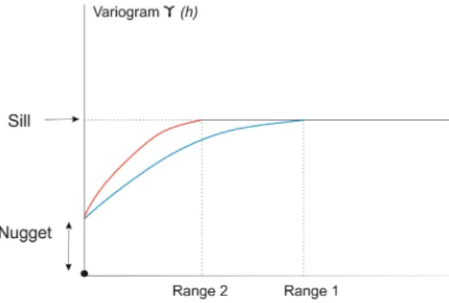
A variogram consists in the study of spatial continuity. It is a mathematical function defined to represent the level of linear dependence between random variables as a function of the distance and direction between the sampled points (Verfaillie et al., 2006). Figure 1 shows the main parameters explained by the experimental semivariogram:
• Range, distance in the variogram in which samples
become independent;
• Sill, semivariogram value corresponding to its range. It reflects the proper dispersion (variance) of the variable for distances superior to the range;
• Nugget effect, quota of the point in which the semivariogram intersects the vertical axis. It reflects microstructures and small-scale variability that are not detected by the sampling. It also reflects sampling errors.
Figure 1 – A hypothetical semivariogram in two directions and the corresponding
parameters.
The extent of the correlation between samples decreases as the distance between them increases. This stage of spatial continuity analysis is one of the most important in geostatistical studies, since it is used for calculating the final estimates map, directly influencing the kriging results.
Interpolation with kriging and cokriging
Kriging is a technique for estimating values in non-sampled locations, through the linear combination of known values, utilizing weights. The result is the construction of an image of the phenomenon that honors the sampling points and guarantees a minimal variance of estimation error in non-sampled locations. It is classified in two forms:
(1) Kriging: the values have the same attribute; (2) Cokriging: values with different attributes are used.
LVM and collocated cokriging methods, are techniques used in multivariate geostatistics applications for the integration of data from different attribute types, described below, were used in this study.
Simple Kriging with LVM
This technique is applied when the secondary variable is exhaustive and is sampled in the whole region. LVM is a simple
kriging in which the average value of the system is replaced by a value contained in the place to be estimated. Thus, the secondary variable must be in the same unit of the primary data. Otherwise, it is necessary to unify the measures through the calibration process, which consists in applying a regression function for converting the secondary data to the unit of the primary data.
Figure 2 presents the parameters of a given place for the LVM system in profile. According to Doyen (2007).
Figure 2 – LVM kriging scheme (Doyen, 2007).
where,
• x(u), defines the primary variable, given by: x(u) = m(u) + R(u)
• m(u), is the local average value, being: E{x(u)}
• R(u), residue between the primary and secondary variables, given by: E{R(u)}
R(u) is stationary and characterized by the covariance CRR(h).
The local estimate in LVM Cokriging consists of mapping the residuals by the linear kriging system and adding the mean given by the secondary variable.
For example, considering primary information sampled in n number of uαlocals:
{z(uα), α= 1, ..., n} (1)
In LVM, secondary information is present in each u local for which it is necessary to have an estimate. Then, the stationary average of the simple kriging system in the u position can be replaced by non-stationary local averages given by the secondary variable m*: Zlvm∗ (u) − m ∗(u) = n(u)
∑
α=1 λα· [Z(uα) − m ∗(u α)] (2)The estimated value of the Z variable in the u position follows the stages below:
(1) the average of the primary variable is determined as a function of the y secondary variable:
m∗(u) = f (y(u)) (3) (2) the kriging weights are determined by solving the system:
n(u)
∑
β=1 λβ·CR(uα− uβ) = CR(uα− u), α= 1, ..., n(u), (4)where, CR(h) is the covariance function of the R(u) random residual variable;
(3) the experimental residues are determined: r(uα) = z(uα) − m
∗
(uα) (5)
(4) the variogram of the residues is calculated; (5) the variogram of the residues is modeled; (6) the residues are estimated by means of kriging;
(7) the result is obtained by adding the average of the secondary variable to the residue estimates.
Collocated Simple Cokriging (CKCS)
The cokriging technique is the extension of the kriging method that adds auxiliary variables in the resolution of the linear system. For instance, if a seismic variable (Z2) with n2points distributed in uα2locals is spatially added to the set of the primary variable (Z1), in the uα1 positions, then the equation of the simple cokriging system (CKS) for estimating the primary variable in any location is given by: ZCKS∗ (u) − m1= n1(u) ∑ α 1=1 λα1· [Z1(uα 1) − m1] + n2(u) ∑ α 2=1 λα2· [Z2(uα 2) − m2] (6)
The weights of simple cokriging are calculated by the system of equations: n1(u) ∑ β 1=1 λβ 1·hC11(uα 1− uβ 1) i + n2(u) ∑ β 2=1 λβ 2·hC12(uα 1− uβ 2) i = C11(uα 1− u) n1(u) ∑ β 1=1 λβ 1· h C21(uα 2− uβ 1) i +n2(u)∑ β 2=1 λβ 2· h C22(uα 2− uβ 2) i = C21(uα 2− u) (7) In matrix form: C11(uα1− uβ1) C12(uα1− uβ2) C21(uα2− uβ 1) C22(uα2− uβ2) · λβ 1 λ β 2 = C11(uα 1− u) C21(uα 2− u) (8)
A practical problem in the use of cokriging is the need to model the covariance matrix for each variable and the cross-covariance between variables. Another problem is how exhaustively sampled the secondary variable is, with much more data than the primary variable, including in places where primary data is available. This makes the cokriging system matrix unstable for greater covariances between secondary values, due to the proximity between them, and lesser covariances between primary data, that are farther apart. The solution for the instability problems caused by highly redundant secondary information consists in retaining in each place of the estimate only secondary data. Thus, the primary variable estimate is given by the collocated cokriging equation, given as:
Z∗ CKCS(u) − m1= n1(u)
∑
α1=1 λα1· [Z1(uα1) − m1] + +λα2· [Z2(u) − m2] (9)Weights are obtained through the following system of equations: C11(uα1− u) = n1(u)
∑
β1=1 λβ1· [C11(uα1− uβ1)]+ +λβ2· [C12(uα1− u)] C21(0) = n1(u)∑
β1=1 λβ1· [C21(u − uβ1)]+ +λβ2· [C22(0)] . (10) In matrix form: C11(uα1− uβ1) C12(uα1− u) C21(u − uβ 1) C22(0) · λβ 1 λβ 2 = C11(uα 1− u) C21(0) (11)The variance of simple collocated kriging being given by: σCKCS2 (u) = C11(0) −
n1
∑
α1=1
λα1·C11(uα1− u) −λα2·C21(0) (12) The CKCS estimating process is very similar to full cokriging system, using only secondary samples located in the point of the estimation. Therefore, the CKCS system needs a covariance between secondary data in estimation points, which decreases the inference and modelling efforts, simplified through Markov models (Goovaerts, 1997).
In Markov models, spatial continuity between primary and secondary variables is approximated by the linear relation of its covariances, given by:
C12(h) =C12(0)
C11(0)C11(h)
In terms of correlation coefficients, it is as follows:
ρ12(h) =ρ12(0) ·ρ11(h) (14) The primary variable estimate is given by the linear regression:
Z1(u) =ρ12(0) · Z2(u) + R(u) (15)
When the variographic models relate to the primary variable, the MM1 model is obtained. When they are a function of the secondary variable, the Markov MM2 model is obtained. For example, the MM2 model is applied in the oil exploration scenario in which primary data is scarce, located in few fields, and secondary data is densely sampled, for instance a seismic cube.
RESULTS AND DISCUSSIONS Exploratory analysis
The first step for exploratory analysis was the elaboration of 1D models of pore pressure gradients for each of the studied wells. For that purpose, pore pressure information from the wells under examination has been compiled. Currently, a well-known approach consists in estimating pore pressure from well logs. However, the thick carbonate platform rocks overlaying
the anomalously pressurized siliciclastic interval makes quite challenging the pore pressure estimation based mainly on well logging data. For that reason, only the pore pressure information recorded at the wells during drilling was taken into account.
As a second step, the top of the abnormal pressure zone (APZ) and the stratigraphic interval of interest were defined. The study emphasized pore pressure anomalies and zones prone to operational risks.
The interval of interest, interpreted as an abnormal pressure zone (APZ), is shown in Figure 3. In this figure, it is possible to observe the abnormal pore pressure behavior in three wells in the area. The abnormal pressure zone is highlighted in green and was interpreted as a predominantly clayey interval, situated below the carbonate platform and reaching about 12,000 psi, 17 lb/gal on well A, 19 lb/gal on well C and 16 lb/gal on well D of equivalent mud weight.
The interval velocity data extracted from the 2D seismic sections was used as a second variable to increase the accuracy of the stochastic model in places lacking well information. The comparison between the interval velocity from well data (projected on seismic sections) and the interval velocity from seismic data can be seen in Figure 4. The curves below show a satisfactory correlation between these parameters in the interval of interest, starting around 3,300 meters (MD) for A and 3,900 meters (MD) for D. The information above these tops, which
Figure 4 – Velocity analysis from wells and 2D seismic lines.
corresponds to a carbonate zone, was not considered in this study.
Considering that there is a relation between the predicted variable (e.g. pore pressure and interval velocity from wells) and a secondary variable (e.g. interval velocity from seismic), it is possible to use multivariate geostatistical tools by including this secondary information into the interpolation. Currently, 3D seismic data are used to increase map resolution, being used to improve the reservoir characterization (Xu et al., 1992). Due to this, a 3D interval velocity cube was estimated from the 2D seismic sections, by means of simple kriging. The advantage of the densely sampled velocity cube is the possibility of extracting pore pressure information at any place on the cube. After that, the histogram analysis of velocity data from seismic and velocity data from wells shows a similar distribution, interpreted as close to a Gaussian one, as can be seen in Figures 5 and 6.
The scatter plot Vp versus pore pressure as recorded in the wells A, C, D and E (Fig. 6) shows two different trends in the same stratigraphic interval: one associated with low velocities varying from 2,000 m/s to 4,000 m/s and higher pore pressures from ~4,3x10³psi to ~13x103psi in the wells A, C and D, and other one associated with higher velocities (around 4,000 m/s) and lower pore pressures (typically below 4,000 psi), the normal pore pressures expected for this area as recorded in well E. It is expected that, according to depth, elastic wave velocities in rocks increase and transit time decreases due to porosity
reduction. In other words, both vary predictably according to depth. However, if there are significant changes in the behavior of these variables, such as a decrease in velocity, it possibly marks a geopressured zone occurrence, once by Sayers et al. (2006). Due to an increase in pore pressure, the amount of compaction can be reduced, allowing the use of elastic wave velocities to predict pore pressure.
Variogram analysis
The theoretical variogram of the 3D velocity cube has been best modeled at azimuthal directions 0° and 90°. This variogram surface shows a clear gaussian type in both directions, reach of 1,000 m and 700 m, nugget effect of 10,000 and 100 and sill with 150,000 and 80,000, respectively at azimuthal directions 0° and 90° (Fig. 7).
This variogram shows that the spatial variation is zonal, the main and secondary directions do not reach the same level. The direction with greater continuity is azimuthal 90°, which corresponds to the direction of faults, probably indicating an influence of the faults in the special variability of the pore pressure data.
Multivariate Interpolation with LVM and Collocated Cokriging
The resulting pore pressure map used pore pressure information from the wells as a predicted variable and a pore pressure
Figure 5 – Histogram of the data set of interval velocity from estimated seismic cube and velocities from wells. Sonic velocity
data were not edited and some spurious values (above ~7,000 m/s) should be disregarded.
Figure 6 – Scatter plot of Vp X pore pressure into the siliciclastic interval (interest interval) from wells data.
cube estimated from the interval velocity cube from seismic data as secondary information. For the calculation of the final pore pressure map and data integration for cokriging, the variogram parameters were used.
Multivariate geostatistical interpolation techniques allowed data integration in spite of the different scales and produced a high-quality pore pressure map, predicting values at unsampled places. There are uncertainties associated with the interpolated
values, but these techniques provide the possibility of extracting pore pressure information at any location in the area, even in places that lack samples.
The results of two multivariate geostatistical tools have been compared in this study: LVM (non-stationary) and collocated cokriging. The LVM technique was able to generate a detailed estimation of the final geopressure cube, with 3,600 km² (Figure 8).
Figure 7 – Horizontal semivariograms at the main and secondary directions.
Figure 8 – Pore pressure estimated using LVM techniques. Figure 9 – Pore pressure estimated using collocated cokriging.
Comparing and validating the final model, as shown in Figure 9, it is possible observe the estimated pore pressure behavior by using collocated cokriging.
For spatial distribution analysis and a better view of pore pressure occurrence, 2D sections within the interval of interest were made. Figure 10 shows two W-E sections, in which the abnormal pressure zones estimated using LVM and collocated cokriging are presented.
The interpolation made through the LVM (non-stationary) approach shows a more detailed estimative of the geopressured cube, while cokriging results leads to a smoother model due to
the applied weights on the primary and secondary variables. For this reason, collocated cokriging conceals relevant information that is otherwise relevant with other estimation techniques. On the other hand, LVM estimative are an important tool in cases where little information is available and detailed information of any variable is necessary, honoring the values of the primary variable. For the same interval, LVM shows a higher pressure in the platform region, as expected from well data analysis. Compared to traditional kriging methodologies, which consider a unique variable, these tools present considerable advantages and more accurate estimations due to the use of secondary variables,
Figure 10 – Pore pressure analysis along the section generated using: (1) LVM estimation and (2) collocated estimation.
especially when only sparse observations are available as is common ground in exploration settings with just a few drilled wells.
CONCLUSIONS
A case study is presented of this being applied on the equatorial margin of Brazil. For the geostatistical analysis the software Petrel (2020) was used and proved satisfactory for all estimates performed in this study.
Multivariate geostatistical techniques are promising tools for obtaining high-quality maps of pore pressure distribution and are fast and robust. The estimations can only be calculated
through well information but merging them with seismic data provide a more accurate geopressured fields model, increasing their resolution.
Due to the satisfactory correlation between the predictive and secondary variables, it was possible to make the LVM and collocated estimation. Comparing the resulting maps, it becomes clear that the LVM estimate showed the best interpolation, presenting more detailed and realistic maps with better resolution. On the other hand, collocated cokriging showed smoother map with lesser resolution. In both cases, the resulting map showed high pore pressure in the interval of interest. This interval is embedded in a Upper Cretaceous thick clay section
in an exploration area on the equatorial margin of Brazil. On the platform region, there are known intervals with anomalous pore pressure fields. The complex tectonic environment of this equatorial margin can be the triggering mechanism for these pore pressure anomalies. The wells used in this work are positioned close to a complex structural distensive/compressive system thus this mechanism was interpreted as the main cause for the high pore pressure anomalies in the area.
ACKNOWLEDGEMENTS
The authors would like to thank WesternGeco for supplying the seismic data, ENAUTA and ANP for allowing the publication of this paper and UFF for all contributions for this study.
REFERENCES
DOYEN PM. 2007. Seismic Reservoir Characterization Geostatistics: An Earth Modelling Perspective. European Association of Geoscientists & Engineers, The Netherlands. 253 pp.
GOOVAERTS P. 1997. Geostatistics for Natural Resources Evaluation. Oxford University Press, New York. 483 pp.
PETREL. 2020. Petrel E&P software platform. Schlumberger. Available on: <https://www.software.slb.com/products/petrel>. Access on: Jan. 2, 2020.
SAYERS CM, DEN BOER LD, NAGY ZR & HOOYMAN PJ. 2006. Well-constrained seismic estimation of pore pressure with uncertainty. The Leading Edge, 25(12): 1524–1526.
VERFAILLIE E, LANCKER VV & MEIRVENNE MV. 2006. Multivariate geostatistic for the predictive modelling of the surficial sand distribution in shelf seas. Continental Shelf Research, 26: 2454-2468.
XU W, TRAN TT, SRIVASTAVA RM & JOURNEL AG. 1992. Integrating seismic data in reservoir modeling: The collocated cokriging alternative. In: Annual Technical Conference of The Society of Petroleum Engineers. 67., SPE-24742-MS, Washington, 1992. p. 833-842.
Recebido em 21 de outubro de 2019 / Aceito em 3 de janeiro de 2020 Received on October 21, 2019 / Accepted on January 3, 2020