Mission Planning Application Software for Solar Powered UAVs

(1)

UNIVERSIDADE DA BEIRA INTERIOR

Engenharia

Mission Planning Application Software for Solar

Powered UAVs

(Versão corrigida após defesa de dissertação)

Pedro Rodrigues Nunes

Dissertação para obtenção do Grau de Mestre em

Engenharia Aeronáutica

(Ciclo de Estudos Integrado)

Orientador: Prof. Doutor Pedro Vieira Gamboa

(2)

(3)

Aos meus pais, Fernando e Assunção. À minha irmã, Inês, e a todos os que permaneceram.

(4)

(5)

Acknowledgments

This thesis is the culmination of five wonderful years at University of Beira Interior, and the product of eight months of research and work. Good and bad times, I experienced them always with the support and company of my family, friends and teachers, and I am forever grateful for them, not only for this period of my life, but for the last five years.

I would like to thank my PhD advisor professor Pedro Vieira Gamboa, from the Department of Aerospace Sciences at UBI, for his readiness in supporting me whenever I had problems, and steering me in the right direction, all the while always letting me do my own work.

I would also like to thank my friends, old and new, for giving me comfort, fun and happiness throughout this time, while also motivating me to keep up the hard work.

Lastly, I would not have the chance to be at this stage without my parents, sister and rest of my family. They get the credit and respect, for my education, for my growth, and for letting me be the person I am now. A big thank you.

(6)

(7)

Resumo

A crescente procura por veículos aéreos não tripulados (UAV) para uso civil na última década tem atraído a atenção de investigadores e engenheiros um pouco por todo o mundo. É importante realçar que a sua desnecessidade de pilotagem manual é idealmente adequada à realização de missões “sujas”, perigosas, monótonas (longa autonomia) ou de grande escala (uso de “enxames” de UAVs) [1], contudo exige uma maior atenção ao desenvolvimento de tecnologias que permitam e facilitem o planeamento, operação e gestão destes veículos. Bastantes avanços têm sido feitos em UAVs movidos a energia solar, que prometem uma operação de baixo custo energético, silenciosa e limpa. Contudo, por mais que a energia solar seja livre e abundante, o presente custo, complexidade, eficiência dos sistemas de captação solar, do armazenamento e da tração usando energia elétrica, bem como a consequente necessidade de veículos de grande tamanho, restringe muito a aplicação extensiva destes veículos [2], para além das dificuldades acrescidas pela ausência de um piloto humano. Não obstante, esta dissertação abrange o desenvolvimento de um interface gráfico de utilizador (GUI) associado ao aperfeiçoamento de um software de planeamento de missões criado a partir de projetos passados, aliando a flexibilidade e rapidez à eficiência de planeamento da operação de UAVs solares. Para além de facilitar a introdução de dados necessários à otimização de uma rota predefinida, este interface permite exportar a rota otimizada para o programa open-source de estação de controlo de solo (GCS) “MissionPlanner” (MP) [3]. Para além disso, o software conjunto final foi também executado como parte de um teste exaustivo, provando as suas capacidades e limitações numa situação real de operação.

Palavras-chave

Veículos Aéreos Não-Tripulados, Planeamento de missões, Operação de UAVs solares, ArduPlane, ArduPilot, Autopiloto

(8)

(9)

Abstract

The growing demand for unmanned aerial vehicles (UAV) for dedicated civilian use over the last decade has attracted the attention of investigators and engineers all over the world. It is important to note that the non-necessity of manual piloting is ideally suited to the operation of dirty, dangerous, dull (long autonomy) or large scale missions (use of swarms of UAVs) [1], however it demands a greater level of attention to the development of technologies that allow and ease the planning, operation and management of such vehicles. A lot of improvement has been made in the development of solar-powered UAVs, which promise a low-energy cost, silent and clean operation. However, despite solar energy being free and abundant, among many the present cost, complexity, solar energy capture systems’ efficiency, electric storage and traction efficiency, as well as the consequent requirement for large-size vehicles, greatly restricts the extensive use of these UAVs [2], besides the added difficulties from the absence of a human pilot. Nevertheless, the present work covers the development of a graphical user interface (GUI) associated to the improvement of a mission planning software created by past work, allying flexibility and quickness to the planning efficiency of solar UAV operations. Beyond facilitating the input of necessary data to the optimization of a pre-set route, this interface allows to export the optimized route to the open-source ground control station (GCS) program “MissionPlanner” (MP) [3]. In addition, as part of an exhaustive testing process, the final ensembled software was run several times, proving its capabilities and limitations in a real operational situation.

Keywords

Unmanned Aerial Vehicles, Mission Planning, Operation of solar UAVs, ArduPlane, ArduPilot, Autopilot

(10)

(11)

List of Figures

Figure 1 – First LEEUAV prototype [4] ... 1

Figure 2 – Sousa’s Solar module attached to the LEEUAV wing prototype [5] ... 2

Figure 3 – Improved LEEUAV fuselage, tail boom and tail control surfaces made by Duarte [6] 2 Figure 4 – Parada’s new V-tail LEEUAV design [7] ... 2

Figure 5 – Sunrise I (1974) and Sunrise II (1975) ... 6

Figure 6 – Solar One (1978) and Solar Riser (1979) ... 6

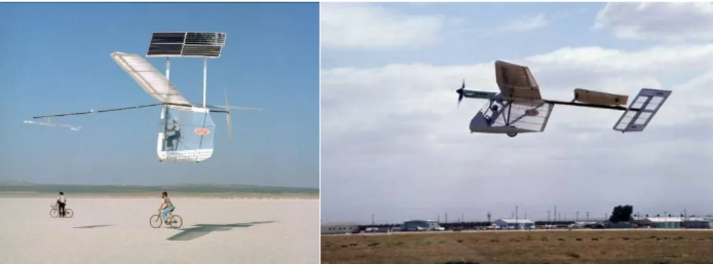
Figure 7 – Gossamer Penguin (1980) and Solar Challenger (1981) ... 7

Figure 8 – Solar Impulse 1 (2011) and Solar Impulse 2 (2014) ... 7

Figure 9 – NASA Pathfinder (1997), Centurion (1998) and Helios (2001) ... 8

Figure 10 – Solong and Zephyr (2005) ... 9

Figure 11 – Sky-Sailor prototype in flight (2008) ... 9

Figure 12 – Solara 50 (concept design) and Aquila (prototype, 2016) ... 10

Figure 13 – Zephyr S prototype before launch (2018) ... 10

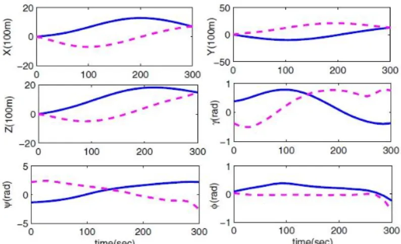
Figure 14 – Dai et al. simulation result example - time history of 3D flight state and control variables from BNB (solid line) and NLP (dash line) [39]... 11

Figure 15 – Example of a 2D path energy-optimization for a mission of ground target tracking [40] ... 12

Figure 16 – Test result of fixed target tracking path of UAV in 3D space [41] ... 12

Figure 17 – Cloud coverage map containing mission areas (MA) and locations of interest (LOI) where the UAV will perform surveillance within a time frame, in the MMS application test [42] ... 13

Figure 18 – The AtlantikSolar prototype (2015) ... 13

Figure 19 – GUI window of the Atlantiksolar path planning and analysis software MetPASS [45] ... 14

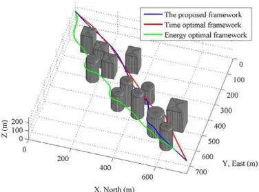
Figure 20 – 3D path planning example of a solar UAV in an urban environment. The “proposed framework” consists of a faster-converging optimization process [47]... 15

(16)

Figure 21 – An example of a QBase 3D route planning ... 16

Figure 22 – QGroundControl mission planning example ... 16

Figure 23 – Example of MissionPlanner route planning ... 16

Figure 24 – The basic structure of the Mission Planner Program [11] ... 19

Figure 25 – Example of a point P (centre) obtained by the interpolation of four coordinates (“Q” dots) [11] ... 21

Figure 26 – Flowchart of the iterative process [11] ... 24

Figure 27 – Flowchart of the iterative process of the FFSQP algorithm [11] ... 26

Figure 28 – Breakdown of the directory structure of the Mission Planner Program ... 29

Figure 29 – Areas of the GUI main window: menu bar (top, red), tab widget (centre, green) and bottom section (bottom, blue) ... 32

Figure 30 – Interface File menu ... 32

Figure 31 – Interface Edit menu ... 33

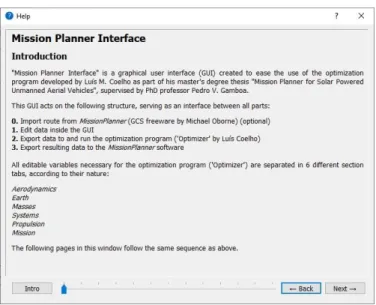
Figure 32 – Introduction page of the “Help” window ... 34

Figure 33 – Bottom section of the interface ... 34

Figure 34 – GUI’s Aerodynamics section tab ... 35

Figure 35 - Aerodynamics/Geometry export operation flowchart ... 36

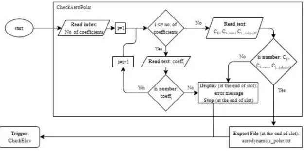
Figure 36 – Aerodynamics/Drag Polar export operation flowchart ... 37

Figure 37 – Design of the Earth tab in the interface ... 37

Figure 38 – Earth/Elevation export operation flowchart ... 38

Figure 39 – Closeup of the lower part of the GUI’s Weather Data section ... 39

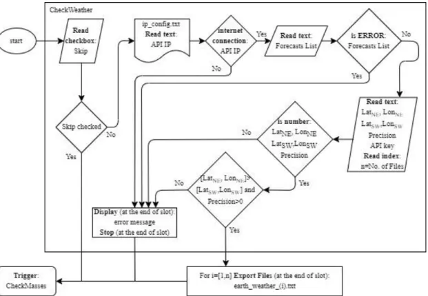
Figure 40 - Earth/Weather export operation flowchart ... 41

Figure 41 – Design of the Masses tab in the interface... 41

Figure 42 - Masses export operation flowchart ... 42

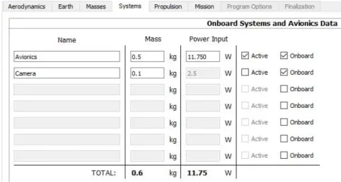
Figure 43 - Design of the Systems tab in the interface ... 43

Figure 44 – Systems export operation flowchart ... 43

(17)

Figure 47 – Propulsion/Battery export operation flowchart ... 46

Figure 48 – Closeup of the Engine/Motor upper part ... 46

Figure 49 – Closeup of the Engine/motor lower part. The left section shows combustion piston engine data, while the right section shows electric motor data ... 47

Figure 50 - Propulsion/Engine export operation flowchart ... 48

Figure 51 - Closeup of the Propulsion/Propeller section ... 48

Figure 52 – Linear interpolation of data points, in the Propulsion/Propeller section ... 49

Figure 53 – Least squares polynomial approximation of data points, in the Propulsion/Propeller section ... 49

Figure 54 – Polynomial representation from user coefficients, in the Propulsion/Propeller section ... 50

Figure 55 – User polynomial curves representation, in the Propulsion/Propeller section ... 50

Figure 56 - Propulsion/Propeller export operation flowchart ... 51

Figure 57 - Design of the Mission tab in the interface ... 51

Figure 58 - Closeup of the Mission/Route and Waypoints upper section ... 52

Figure 59 – Example of a route in the GEO coordinates waypoints table ... 53

Figure 60 – Same route as in figure 59, ENU coordinates waypoints table ... 53

Figure 61 – Closeup of the loiters table ... 54

Figure 62 – Mission/Route and Waypoints export operation flowchart #1 ... 55

Figure 63 - Mission/Route and Waypoints export operation flowchart #2 ... 56

Figure 64 – Expanded view of the Mission/Optimization section. Outlined are the optimization options (pink), design parameters stack widget (green), objective function (red), equality constraints (blue) and inequality constraints (yellow) ... 57

Figure 65 – Expanded view of Latitude design parameter table (similar to longitude, altitude and airspeed tables) (upper) and mission initial hour design parameter table (lower) ... 58

Figure 66 – Mission/Optimization export operation flowchart ... 59

Figure 67 – Closeup of the Mission/FFSQP section ... 60

(18)

Figure 69 – Example of an error box showing the affected section ... 62

Figure 70 – “Export Files” slot operation flowchart ... 63

Figure 71 - GUI’s Program Options tab ... 64

Figure 72 – GUI’s Finalization tab ... 65

Figure 73 – Example of a 5-waypoint route in MissionPlanner ready to be exported to the GUI ... 67

Figure 74 – Example of a converted route in MissionPlanner. Highlighted are the DO_SET_HOME command (red), the TAKEOFF and LAND commands (green), and the example of a waypoint (blue) with loiter commands (yellow) ... 68

Figure 75 – List of commands of the input route in the MissionPlanner ... 70

Figure 77 – Top-down map view of the route in MissionPlanner ... 71

Figure 76 – View of input route data in the GUI’s Mission tab ... 71

Figure 78 – 3D view of the terrain map and input route ... 72

Figure 79 – Side view of the terrain map and input route. Departing point is on the right side ... 72

Figure 80 - Tests’ daily cloud and wind analysis at 9 o’clock. North is to the right side ... 73

Figure 81 - Tests’ daily cloud and wind analysis at 12 o’clock. North is to the right side ... 73

Figure 82 – Running time comparison between different CPUs for the ME optimization tests . 81 Figure 83 – Running time comparison between ME and MT optimization tests for engine-propeller data 1 ... 82

Figure 84 - Theoretical example of a route with 5 waypoints. δj represent the segment flight performance calculated between consecutive waypoints [11] ... 94

(19)

List of Tables

Table 1 – Variables for GEO and ENU waypoint tables ... 54

Table 2 – Modes of Optimization values table ... 60

Table 3 – Waypoints table of the input route ... 70

Table 4 – Loiters table of the input route ... 70

Table 5 – LEEUAV Motor Data ... 74

Table 6 – LEEUAV Propeller Data ... 75

Table 7 – LEEUAV Aerodynamics-Geometry Data ... 75

Table 8 - LEEUAV Aerodynamics-Drag Polar Data ... 75

Table 9 – LEEUAV Aerodynamics-Aircraft Representation data ... 75

Table 10 – LEEUAV Masses Data... 75

Table 11 – LEEUAV Systems Data ... 76

Table 12 – LEEUAV Battery Data ... 76

Table 13 – Inequality constraint functions used during the optimization tests ... 76

Table 14 – Lower and Upper bounds used during the optimization tests for the design parameters ... 77

Table 15 – Codes to organize the tests ... 77

Table 16 – Engine-propeller type 1, Minimize Energy (E1-ME) test results ... 78

Table 17 – Engine-propeller type 2, Minimize Energy (E2-ME) test results ... 78

Table 18 - Engine-propeller type 1, Minimize Time (E1-MT) test results ... 80

(20)

(21)

List of Acronyms

AEROG Aeronautics and Astronautics Research Centre (UBI)

API Application Programming Interface

CCTAE Centro de Ciências e Tecnologias Aeronáuticas e Espaciais (IST)

CPU Central Processing Unit

DLR German Aerospace Centre

EADS European Aeronautic Defence and Space Company (Astrium)

ENU East-North-Up coordinates system

ERAST Environmental Research Aircraft and Sensor Technology (NASA)

ESC Electronic Speed Controller

ETHZ Swiss Federal Institute of Technology Zurich

FAI Fédération Aéronautique Internationale

FFSQP Fortran Feasible Sequential Quadratic Programming

GCS Ground Control Station

GEO Geodetic coordinates system

GPL General Public License

GUI Graphical User Interface

HALE High Altitude Long Endurance

HALSOL High Altitude Solar

IDMEC Instituto de Engenharia Mecânica (IST)

INEGI Instituto de Ciência e Inovação em Engenharia Mecânica e Industrial

ISA International Standard Atmosphere

IST Instituto Superior Técnico

LAETA Laboratório Associado de Energia, Transportes e Aeronáutica LEEUAV Long Endurance Electric Unmanned Aerial Vehicle

MDP Markov Decision Process

MetPASS Meteorology-aware Path Planning and Analysis software for Solar-

powered UAVs (Atlantiksolar)

MMS Mission Management System

MP MissionPlanner (open-source software by Michael Oborne)

MPP Mission Planner Program

MSL Mean Sea Level

NASA National Aeronautics and Space Administration (USA)

PV Photovoltaic

RC Radio-controlled

R&D Research and Development

(22)

SQP Sequential Quadratic Programming

UAS Unmanned Aerial System

UAV Unmanned Aerial Vehicle

UBI Universidade da Beira Interior

URL Uniform Resource Locator (web address)

(23)

Nomenclature

ROMAN SYMBOLS 𝐴̅,𝐵̅ ,𝐶 ̅,𝐷̅ ,𝐸̅ Coefficient vectors 𝐶_{𝑏𝑎𝑡𝑡} Battery capacity [𝐴ℎ] 𝐶_{𝑐𝑒𝑙𝑙} Cell capacity [𝐴ℎ] 𝐶_𝐷 Drag coefficient

𝐶𝐹 Fuselage skin friction coefficient

𝐶𝐿 Lift coefficient

𝐶𝐿_𝑚𝑎𝑥 Maximum lift coefficient

𝐶_𝐿

𝑡𝑎𝑘𝑒𝑜𝑓𝑓 Take-off lift coefficient

𝐶𝑝 Power coefficient

𝐶𝑝,0 Power coefficient at null advance ratio

𝑑 Propeller diameter [𝑚]

𝑑𝑛 Day of the year

𝐸 Mission consumed energy [𝐽]

𝐸_{𝑙𝑒𝑓𝑡} Battery energy left [𝐽]

𝐸_𝑟𝑒𝑓 Battery energy left constraint reference value

𝐸_{𝑠𝑜𝑙𝑎𝑟|𝑡𝑜𝑡𝑎𝑙} Total solar energy harvested by photovoltaic panels [𝐽] 𝑓𝑜𝑟𝑒𝑓𝑖𝑛𝑎𝑙 Mission final weather forecast hour [ℎ]

𝑓𝑜𝑟𝑒𝑖𝑛𝑖𝑡 Mission initial weather forecast hour [ℎ]

𝑓𝑜𝑟𝑒𝑛𝑜𝑤 Current weather forecast hour [ℎ]

𝐻 Hour of the day [ℎ]

ℎ Altitude [𝑚]

ℎ𝑟𝑒𝑓 Reference altitude [𝑚]

𝐼 Input current [𝐴]

𝐼0 No load current [𝐴]

𝐼𝑏𝑎𝑡𝑡_𝑚𝑎𝑥 Maximum battery current [𝐴]

𝐼_{𝑐𝑒𝑙𝑙}

𝑚𝑎𝑥 Maximum cell current [𝐴]

𝐼𝑒𝑓𝑓 Effective input current [𝐴]

𝐼𝑚𝑎𝑥 Maximum input current [𝐴]

𝐼𝑟𝑒𝑓 Reference input current [𝐴]

𝐽 Solar irradiation [𝑊 /𝑚2_]

(24)

𝐾_𝐶 Clear sky index [%]

𝐾_𝑡 Motor torque constant

𝐾_𝑣 Motor speed constant

𝐿𝑎𝑡 Latitude coordinate [𝑑𝑒𝑔]

𝐿𝑜𝑛 Longitude coordinate [𝑑𝑒𝑔]

𝑚𝑏𝑎𝑡𝑡 Battery mass [𝑘𝑔]

𝑚𝑐𝑒𝑙𝑙 Single cell mass [𝑘𝑔]

𝑚𝑒𝑛𝑔 Mass of engine/motor [𝑘𝑔]

𝑚𝑝𝑟𝑜𝑝 Mass of propeller [𝑘𝑔]

𝑁 Propeller/Engine speed [𝑟𝑝𝑚]

𝑁₀ Minimum engine speed at idle throttle [𝑟𝑝𝑚]

𝑁_𝑚𝑎𝑥 Maximum engine speed [𝑟𝑝𝑚]

𝑛 Propeller/Engine speed [𝑟𝑝𝑠]

𝑛_{𝑏𝑙𝑎𝑑𝑒𝑠} Number of propeller blades 𝑛_{𝑐𝑒𝑙𝑙𝑠,𝑝𝑎𝑟𝑎𝑙𝑙𝑒𝑙} Number of battery cells in parallel 𝑛𝑐𝑒𝑙𝑙𝑠,𝑠𝑒𝑟𝑖𝑒𝑠 Number of battery cells in series

𝑛𝑒𝑛𝑔 Number of engines/motors

𝑛𝑤𝑒𝑎𝑡ℎ𝑒𝑟 Number of weather files

𝑝 Propeller pitch [𝑚]

𝑃_𝑒𝑓𝑓 Effective power [𝑊 ]

𝑃_𝑒𝑙𝑒 Electric power [𝑊 ]

𝑃_𝑚𝑎𝑥 Maximum engine power [𝑊 ]

𝑃𝑟𝑒𝑓 Required power reference value [𝑊 ]

𝑃_𝑟𝑒𝑞 Required power [𝑊 ]

𝑃𝑠ℎ𝑎𝑓𝑡 Motor power at the shaft [𝑊 ]

𝑃𝑠𝑦𝑠 Systems power [𝑊 ]

𝑃𝑠𝑦𝑠,𝑒𝑛𝑔 Engine systems power [𝑊 ]

𝑃𝑇 Total electric power [𝑊 ]

𝑄𝐶𝑙𝑜𝑢𝑑𝑠_𝑖 Cloud index [%]

𝑄𝑒𝑙𝑒_𝑖 Elevation value [𝑚]

𝑄𝐸𝑙𝑒𝑣𝑎𝑡𝑖𝑜𝑛 Elevation data

𝑄𝑙𝑎𝑡_𝑖 Latitude coordinates of the elevation/weather map [𝑑𝑒𝑔]

𝑄𝑙𝑜𝑛_𝑖 Longitude coordinates of the elevation/weather map [𝑑𝑒𝑔]

𝑄_{𝑚𝑜𝑡𝑜𝑟} Motor torque at the shaft [𝑁𝑚] 𝑄_{𝑇𝑒𝑚𝑝}

(25)

𝑄_{𝑤𝑖𝑛𝑑𝑑𝑖𝑟𝑒𝑐𝑡𝑖𝑜𝑛}

𝑖 Wind direction [𝑑𝑒𝑔]

𝑄𝑤𝑖𝑛𝑑𝑠𝑝𝑒𝑒𝑑_𝑖 Wind speed [𝑚/𝑠]

𝑅 Electric resistance [Ω]

𝑅_{𝑐𝑒𝑙𝑙} Cell internal resistance [Ω]

𝑅_𝐸𝑆𝐶 Electronic speed controller resistance [Ω]

𝑅_{𝑚𝑜𝑡𝑜𝑟} Motor internal resistance [Ω]

𝑟_{𝑔𝑒𝑎𝑟} Gearbox ratio

𝑅𝑈 Battery resistance [Ω]

𝑆 Wing reference area [𝑚2_]

𝑆𝐹 Fuselage cross-section area [𝑚2]

𝑠𝑓𝑐 Specific fuel consumption [𝑘𝑔/𝑊𝑠]

𝑆𝑃𝑉 Photovoltaic panels area [𝑚2]

𝑆𝑊𝑒𝑡 Fuselage wetted area [𝑚2]

𝑡 Time [𝑠]

𝑡_{𝑓𝑖𝑛𝑎𝑙}

ℎ Mission final hour [ℎ]

𝑡𝑖𝑛𝑖𝑡 Internal mission initial hour [ℎ]

𝑡𝑖𝑛𝑖𝑡_𝑑𝑎𝑦 Mission date day

𝑡𝑖𝑛𝑖𝑡_ℎ Mission date initial hour [ℎ]

𝑡_{𝑖𝑛𝑖𝑡}

𝑦𝑒𝑎𝑟 Mission date year

𝑈 Input voltage [𝑉 ]

𝑈0 No load voltage [𝑉 ]

𝑢𝑏𝑎𝑡𝑡 Battery specific energy [𝑊ℎ/𝑘𝑔]

𝑈𝑏𝑎𝑡𝑡 Nominal battery voltage [𝑉 ]

𝑈𝑏𝑎𝑡𝑡_𝑚𝑎𝑥 Maximum battery voltage [𝑉 ]

𝑈_{𝑏𝑎𝑡𝑡}

𝑚𝑖𝑛 Minimum battery voltage [𝑉 ]

𝑈𝑐𝑒𝑙𝑙 Nominal cell voltage [𝑉 ]

𝑈𝑐𝑒𝑙𝑙_𝑚𝑎𝑥 Maximum cell voltage [𝑉 ]

𝑈_{𝑐𝑒𝑙𝑙}

𝑚𝑖𝑛 Minimum cell voltage [𝑉 ]

𝑈𝑒𝑓𝑓 Effective input voltage [𝑉 ]

𝑈_𝑚𝑎𝑥 Maximum input voltage [𝑉 ]

𝑉 Aircraft linear velocity [𝑚/𝑠]

GREEK SYMBOLS

𝛿𝑙𝑖𝑚𝑖𝑡 Engine/Motor throttle limit

𝛿_𝑠𝑒𝑡 Engine/Motor throttle setting

(26)

𝜂_{𝑝𝑟𝑜𝑝} Propeller efficiency

𝜂_𝑃𝑉 Photovoltaic panels efficiency

𝜃_𝑖 Angle of incidence of the sun [𝑑𝑒𝑔]

𝜆 Longitude [𝑑𝑒𝑔]

𝜌 Air relative density [𝑘𝑔. 𝑚−3_]

(27)

(28)

(29)

Chapter 1

Introduction

1.1 Contextualization

The present work comes in line with the University of Beira Interior (UBI) and Instituto Superior Técnico (IST) recent years’ research and development of a solar-powered Long Endurance Electric UAV (LEEUAV). As many as 8 authors’ thesis were considered as a base of research accomplished so far, and on which this thesis builds on.

The LEEUAV is a particular type of unmanned aerial vehicle (UAV) that was especially designed to fly uninterruptedly for at least 8 hours during the Spring or Autumn equinoxes, while also being able to carry up to 1kg of payload, to take-off and land in a short distance, to climb 1000 meters in 10 minutes, and to descend without power [2]. As an object of research and development (R&D), the LEEUAV project started out as a consortium involving UBI and IST, and whose members include the “Energy, Transportation and Aeronautics Associated Laboratory” (LAETA), namely the “Centre of Aeronautics and Space Sciences and Technologies” (CCTAE), the “Aeronautics and Astronautics Research Centre” (AEROG), the Institute of Mechanical Engineering (IDMEC) and the Institute of Science and Innovation in Mechanical and Industrial Engineering (INEGI). In brief, the line of work started in 2014 with the successful conceptual and preliminary design, and development testing of a newly built prototype, made by Cândido [4].

In 2015, a solar component for the electric propulsion system was added to the wings of the prototype and validated by Sousa [5].

(30)

In 2016, Duarte [6] specifically designed and built a new structural fuselage, tail boom and tail control surfaces for the LEEUAV, in order to withstand missions with payloads up to 1kg.

Also, in the same year, Parada [7] developed a different conceptual and preliminary design for a new LEEUAV, choosing the V-tail airplane concept over the conventional tail configuration.

In 2017, the conventional-tail LEEUAV with the latest fuselage, tail and wings was successfully assembled, tested and modified by Rodrigues [8], following integration of all electronic components, including the repositioning of the solar panels based on the work of Freitas [9]. At the same time, Moutinho designed a real-time energy management system to estimate the remaining flight time, based on the total energy balance, while also developing the data forwarding and receiving to and from the UAV, plus the visualization on the GCS

Figure 2 – Sousa’s Solar module attached to the LEEUAV wing prototype [5]

Figure 3 – Improved LEEUAV fuselage, tail boom and tail control surfaces made by Duarte [6]

(31)

Lastly, in 2019, the work on which this thesis is primarily based, Coelho created a Mission Planner Program (MPP) for a solar powered UAV, using the FFSQP algorithm and taking into account several models for mission planning: UAV performance constraints, ground elevation, atmospheric data and solar panels, sun and vehicle orientation [11].

1.2 Motivation

The reasons to the development of this thesis can be summarized into two main factors: planning for in-flight operational efficiency and flight safety.

Although UAV utilization is soaring all over the world, the bulk of development accomplished so far was made by several military institutions, much like in the earlier days of aviation. Though essential to the general development of the UAV as an airplane class, military development only ensures operations of the kind in the field, and normally prioritises assertion of power over profitability. An efficient planning before a mission ensures the success of a civilian operation, as this kind of operation must have economic viability. The creation and integration of a user-friendly and interactive graphical user interface (GUI) in a mission planner program makes the input process easy, fast and reliable to the user, where many different route optimizations can be made before a mission starts, and the user can choose which route is best to perform a specific mission.

The absence of a human pilot in autonomous UAVs dismisses many assurances normally present in the safe operation of manned aircraft. Human piloting, though many times limiting and disadvantageous, presents many advantages to a safe operation, namely the independent and quick decision making in the event of an emergency, the ability to break rules when needed, to think analytically and creatively to solve unexpected and never-before-occurred problems [12], things an autopilot would not yet be able to do in today’s level of automation. Therefore, safety can be better achieved if the input of data into a mission planning program is correct and good environmental conditions are assured. Again, the development of a clear, understandable and reliable GUI is essential to a safe planned mission.

1.3 Objectives

This thesis follows the line of work of past LEEUAV-related works already mentioned before, in particular that of Coelho [11]. One could consider this thesis to be the second part of the development of a Mission Planner Program (MPP) (not to be confused with “MissionPlanner”, an open-source software developed by Michael Oborne [3]). In essence, the main objectives of the present work can be summarized as follows:

(32)

• Ease the data input, output data retrieval and visual presentation of the MPP, by developing a graphical user interface (GUI), explaining its functioning structure, capacities and limitations;

• Perform various test runs of the ensembled Mission Planner Program, which includes Coelho’s Mission Planner (also referred to as MPP or ‘Optimizer’ throughout this thesis) and the GUI, analyse and compare optimization results. This is done to validate the work developed thus far;

• Draw conclusions and suggestions for future work.

1.4 Thesis Outline

Including the present introductory chapter, this thesis is divided into 6 main chapters, which are briefly described below:

Chapter 1 covers the contextualization, motivation and objectives of the work to be done; Chapter 2 focuses on a historical and state of the art review of the operation and mission path planning of solar-powered UAVs;

Chapter 3 covers the explanation of the Mission Planner Program by Coelho and the addition of new features, such as a new mission initial hour optimization design parameter and modifications to the minimization of energy flow. This chapter is crucial to understanding how the GUI will be added afterwards;

Chapter 4 explains the developing process of the GUI and its functioning structure, as well as a brief explanation of the system of exporting/importing data to/from the MissionPlanner freeware by Michael Oborne;

Chapter 5 describes how various optimization tests of a route from Terlamonte (Covilhã) to Castelo Branco and back were performed, according to a certain objective function, design parameters, and day of operation. Following that, a detailed analysis and comparation of results is made;

Chapter 6 provides the conclusions to draw from this work, as well as what future work could be made to improve planning and operation of solar-powered UAVs and the LEEUAV.

(33)

Chapter 2

State of the Art

2.1 History of solar-powered aircraft

Though aviation has been around since the 19th_{century, solar-powered aircraft operations have} a very recent history. Electric solar propulsion has lagged behind conventional fossil fuels’ propulsion because it is still mainly limited by the current level of development and efficiency of batteries and photovoltaic (PV) cells.

2.1.1 Early developments

The use of electric propulsion for aircraft was first introduced as early as 1884, with the hydrogen-filled dirigible La France. At the time, electric propulsion was superior to its rival, steam propulsion. However, the technology went undeveloped and abandoned for almost a century, in favour of gasoline propulsion [13]. The first officially recorded electric powered radio-controlled flight was achieved on 30 June 1957, with the RC model “Radio Queen”, by UK Colonel H. J. Taplin. Also, in October 1957, German pioneer Fred Militky first achieved a successful flight with a free flight model. Photovoltaic (PV) cells first appeared in 1954 at Bell Telephone Laboratories [14]. However, the technology to harness solar light as energy to viably power an aircraft only really took off in the 1970s.

Starting in 1970, R. J. Boucher and his brother Roland Boucher from Astro Flight Inc. began their experiments with electric flight. On 4 November 1974, Sunrise I, the first ever solar-powered model aircraft, took off from a dry lake at Camp Irwin, California, USA. The Sunrise I had a wingspan of 9.75m and weighed 12.47kg. Following the partial destruction of the airplane in a sandstorm, an improved second model Sunrise II was built and flown on 12 September 1975, at Nellis AFB. Having the same wingspan as its predecessor, the Sunrise II weighed 10.21kg and its 14% efficient PV cells could produce 150W more power than the 450W of Sunrise I. These breakthroughs set the stage for later developments in solar aviation [13].

(34)

At the same time in Germany, Helmut Bruss worked on a solar model airplane, though unsuccessful in achieving level flight. Later on 16 August 1976, his friend Fred Militky first flew his solar-powered Solaris airplane, completing three 150-second flights and reaching an altitude of 50 meters [15].

2.1.2 Manned solar-powered aircraft

The feasibility of solar power in model aircraft motivated its development on manned aircraft. David Williams and Fred To launched the Solar One in Hampshire UK, 19 December 1978. This aircraft was intended to be human powered and cross the English Channel, however it proved too heavy and was thus converted to solar power [13], [16]. On 29 April 1979, Larry Mauro flew the Solar Riser, an electric airplane capable to charge its battery with solar power, but not able to fly longer than ten minutes [13].

Flying on the use of solar power alone without any batteries was first achieved on 18 May 1980 by the Gossamer Penguin, built by Dr. Paul B. MacCready and his company AeroVironment Inc. This was also the world’s first piloted, solar-powered flight. Though the Gossamer Penguin was only able to reach a few meters in altitude, Dr. MacCready also built a new solar airplane, the Solar Challenger, which crossed the English Channel on 7 July 1981, covering 262.3km of distance with only solar energy as its power source and no onboard batteries [13].

Figure 5 – Sunrise I (1974) and Sunrise II (1975)

(35)

Other important late 20th_{century manned solar aircraft developments include Günther} Rochelt’s Solair I, a 16m wingspan solar airplane which flew for 5 hours and 41 minutes in August 1983, Eric Raymond’s Sunseeker, which crossed the continental USA in 21 solar-powered flights and 121 flight hours in August 1990 [17], and Prof. Rudolf Voit-Nitschmann’s Icaré 2 solar-powered motor glider which flew on 7 July 1996 [18].

In 2003, Bertrand Piccard initiated the Solar Impulse project in partnership with the Swiss Institute of Technology in Lausanne (EPFL), to develop long-endurance manned solar-powered aircraft that could circumnavigate the globe. The first prototype, Solar Impulse 1, first flew in December 2009, and performed a multi-stage flight across the USA in 2013. The second-generation aircraft, Solar Impulse 2, was built in 2014. It managed to circumnavigate the globe, starting in Abu Dhabi, 9 March 2015, flying West-to-East and returning on 26 July 2016 [19], [20].

Another solar-powered manned airplane, the two-seater SolarStratos, was built and flown by Raphaël Domjan on 5 May 2017, and is projected to be the first to reach the stratosphere in the very near future [21].

Figure 7 – Gossamer Penguin (1980) and Solar Challenger (1981)

(36)

2.1.3 Long Endurance UAVs

Following the success of the Solar Challenger, AeroVironment Inc. received US government funding to secretly develop a remotely controlled High-Altitude Solar (HALSOL) LEEUAV, and built a prototype in 1983. However, contemporary solar PV and energy storage technologies were not mature enough to allow a HALSOL flight [22]. 10 years later, the prototype was flown again by NASA and was transferred to NASA’s ERAST program in 1994, being renamed Pathfinder. In 1995, it surpassed Solar Challenger’s altitude record, reaching 15392m (50500ft), and two years later it reached 21802m (71530ft). NASA’s Pathfinder was modified into the Pathfinder Plus, having a larger wingspan and new solar, aerodynamic, propulsion and system technologies. Two successor aircraft were followed in NASA’s ERAST program: the Centurion and the Helios. The latter was intended to reach 30480m (100000ft) and fly non-stop for at least 24 hours. It flew at an altitude of 29261m (96000ft) for 40 minutes, was able to carry a payload up to 329kg. Unfortunately, it crashed into the Pacific Ocean before it could validate its 24-hour endurance goal [23].

Meanwhile in Europe, many other projects also started to appear to develop a High-Altitude Long Endurance (HALE) UAV, namely the Solitair, at DLR Institute of Flight Systems (1994-1998) [24], the Heliplat, developed by several European partners (2000-2003) and Shampo, developed by the Politecnico di Torino [25], [26].

On 22 April 2005, Alan Cocconi flew his Solong for 24 hours and 11 minutes using only solar power and wind thermals, finally validating the goal of eternal flight for the first time. Two months later, in the Colorado Desert CA, he managed to perform an even more ambitious flight, which lasted for a total of 48 hours and 16 minutes [17].

Also competing in the solar HALE platforms field, British Defence contractor QinetiQ flew a Zephyr aircraft on 10 September 2007 for a duration of 54 hours, also using solar power and wind thermals only. The aircraft was able to reach an altitude of 17786 meters, weighed 30kg and had a wingspan of 18 meters [27]. Later in 2008, the Zephyr 6 performed an 82-hour flight at an altitude of 19000m, but did not set any records because of the absence of World Air Sports Federation (FAI) officials [28]. The Zephyr was also selected to carry the Mercator remote

(37)

sensing system in 2005, which allows to perform forest fire monitoring, urban mapping, coastal monitoring, oil spill detection, etc.

The Sky-Sailor is another solar-powered LEEUAV project first designed in 2004 by the Swiss Institute of Technology in Lausanne (EPFL) to demonstrate HALE flight, this time for the scientific exploration of Mars. It was designed to be autonomous, to have its flight path planned beforehand and to be able to navigate using range sensors and vision only (as GPS is not available outside of Earth). The prototype’s flight characteristics were successfully tested in June 2008, and it was the first ever to fly continuously for 27 hours without using altitude gain or thermal soaring [29].

An example of recent developments in long endurance UAVs can be found in Titan Aerospace’s Solara 50. This 50-meter wingspan autonomous UAV was designed to function as an atmospheric satellite operating at an altitude of 20km above any possible storms in the troposphere, and able to carry 31.75kg of telecom, reconnaissance, atmospheric sensors or other payloads, while operating as part of a fleet of other UAVs for as long as five years. Titan Aerospace was bought by Google in 2014, however the project was abandoned in 2016. The only built prototype got to fly for 4 minutes and 16 seconds before crashing after an in-flight structural failure on 1 May 2015 [30]–[32].

Another example of an autonomous solar LEEUAV is that of Facebook’s Aquila. It was designed to provide communications service (mainly Internet connection) to remote areas in the world, operating between 18.3km and 27.4km of altitude. The only 42m-wingspan built prototype first

Figure 10 – Solong and Zephyr (2005)

Figure 11 – Sky-Sailor prototype in flight (2008)

(38)

flew in 2016 for an hour and 36 minutes, however the whole program was cancelled by Facebook in 2018, which favoured their partnership with other companies in the field [33]–[35].

The Zephyr program, founded in 2003 by QinetiQ, is still in development today. Recently in the summer of 2018, the new Zephyr S reached an astonishing flight of 25 days 23 hours 57 minutes, doubling the record of 14 days set by its predecessor. This aircraft was designed to provide persistent surveillance in response to a natural or human-caused disaster, or to act as a telecommunications relay station [36].

2.2 Mission Planning

In order to better understand the motivation behind the making of this work, a comprehensive review of recent developments in UAV mission planning techniques and current knowledge must be undertaken.

As seen in the previous section, solar-powered aircraft have come a long way since the first solar models, and a lot can still be done to improve in regards to flight performance. In a way, the very development of the technology to harness the sunlight and convert it to energy is a big game changer in the operation of UAVs in particular, because it allows the vehicle to remain in operation for an indefinite amount of time, if energy storage so allows. With this, a particular range of applications have been improved in Unmanned Aerial Systems (UAS) operations, such as, among others [37]:

Figure 12 – Solara 50 (concept design) and Aquila (prototype, 2016)

Figure 13 – Zephyr S prototype before launch (2018)

(39)

• facilitation of communications and broadcast;

• monitoring of linear network infrastructure (e.g. railway tracks, power lines, pipelines);

• photography and cartographic survey; • atmospheric research.

A lot more solar LEEUAV-related projects will, of course, be started in the very near future, providing ever more knowledge in the art of UAV operation. But most of solar flights in the previous decades were manually planned and performed using the best conditions possible, which is understandable for new experimental aircraft.

Therefore, new and effective mission planning and coordination techniques have also been developed to improve the operation of a solar-powered UAV, even when conditions are not favourable. The use of these techniques allows the optimization of routes, according to goals like: energy usage, travel time or distance minimization; obstacle/collision avoidance; surveillance/coverage time maximization; or endurance/autonomy maximization. Not only by decreasing the amount of consumed energy of the mission, but also by increasing the amount of energy obtained from solar power, the LEEUAV can be operated efficiently and use its capabilities to the fullest possible.

Based on the work of Klesh et al. [38], Dai et al. investigated a unit quaternion-based method used to design the optimal UAV trajectory with maximum sun exposure for solar UAVs. Considering a mission delimited by two boundary points with fixed flying time and constant speed, this work optimizes the route of the UAV by adjusting its attitude – pitch (𝛾), heading (𝜓) and roll (𝜙) angles, subject to constraints – in a level and three-dimensional flight models, using a branch and bound (BNB) and nonlinear programming (NLP) approaches [39]. An example of one of the simulation results is displayed in Figure 14.

Figure 14 – Dai et al. simulation result example - time history of 3D flight state and control variables from BNB (solid line) and NLP (dash

(40)

In 2016, Huang et al. developed an online method to obtain energy-optimal trajectories with the mission of ground target tracking. Although different from missions with no target tracking, this method presents a simple energy integrated model in two-dimensional space to calculate the instantaneous power, collect more energy and track the moving target using the optimization method of receding horizon control (RHC) with particle swarm optimization (PSO) [40]. Several numerical simulations demonstrated the feasibility and flexibility of this method, one of which is shown in Figure 15.

Later in 2019, Huang et al. developed a similar 3D path planning method for solar-powered UAVs, albeit intended for fixed target and solar tracking. Taking into consideration the UAV’s motion and attitude, mission constraints, energy production and energy consumption, the loitering flight paths are planned on a virtual cylinder surface in 3D space, with the fixed target centre at its origin [41]. One of the test results of this method is shown in Figure 16.

The work of Kiam et al., presented in March 2017, demonstrates a multilateral quality mission-planning tool to increase the endurance of solar-powered LEEUAVs. The focus of the tool is set on very-long endurance missions, such as surveillance, using high-altitude pseudo satellites (HAPS fixed-wing UAV platforms) on certain locations of interest (LOI). It uses a highly automated mission management system (MMS) which produces an optimal plan subject to the

Figure 15 – Example of a 2D path energy-optimization for a mission of ground target tracking [40]

Figure 16 – Test result of fixed target tracking path of UAV in 3D space [41]

(41)

constraints. This MMS adopts the hybrid architecture of a symbolic planner based on the hierarchical task-network (HTN), working with a Markov decision process (MDP) based policy generator to reduce the search space for a numerical path planner [42].

A new solar LEEUAV dubbed AtlantikSolar by its developer, the Swiss Federal Institute of Technology at Zurich (ETHZ), has been developed since 2015 to fly autonomously in Low-Altitude Long Endurance (LALE) missions, for applications such as industrial and agricultural sensing and mapping, large-scale disaster relief support missions, meteorological surveys in remote areas and continuous border or maritime patrol. It was especially designed with efficient autonomous path planning and operation in mind [43], [44].

The software responsible for this autonomous path planning is the MetPASS – Meteorology-aware Path Planning and Analysis Software for Solar-powered UAVs. It consists of an optimization software that combines an A* algorithm, a dynamic programming point-to-point planner and a local scan path planner (a simple camera model), to yield cost-optimal aircraft paths. The cost function considers both safety and performance variables, such as terrain collision risk, system state (time since launch, battery state of charge, power consumption and generation) through a comprehensive energetic model, and meteorological data (thunderstorms, precipitation,

Figure 18 – The AtlantikSolar prototype (2015)

Figure 17 – Cloud coverage map containing mission areas (MA) and locations of interest (LOI) where the UAV will perform surveillance within

(42)

humidity, 2D winds, gusts, sun radiation and clouds) through global weather models. Furthermore, the MetPASS was fully implemented with a GUI that allows an easy-to-use, detailed mission feasibility analysis, pre-flight planning and in-flight re-planning using updated weather data. Several real flight tests (a loitering 81-hour endurance flight in June 2015 and a series of Arctic glacier multi-goal survey flights in July 2017) were performed for the validation of the MetPASS. It was also validated through extensive testing for the planning of a 4000km crossing of the Atlantic Ocean, from Newfoundland to Portugal, the flight of which is yet to take place [45].

In 2018, Amorosi et al. developed an energy-efficient mission planning method intended for 5G network coverage in rural zones (using a swarm of non-solar-powered UAVs), by solving the “RURALPLAN” optimization problem, a variant of the unsplittable multicommodity flow problem defined on a multiperiod graph. Not only this method limits the amount of energy consumed above minimum battery level constraints, it also ensures the coverage of selected zones and determines sites where an UAV should land to recharge, considering the amount of energy provided by the PV panels and batteries installed at those ground sites [46]. Although not intended for the operation of solar-powered UAVs, future work on this method using an onboard solar component would ensure greater endurance performance, proving to be particularly useful at Winter days.

Another work, presented by Wu et al. in the same year, shows the development of a

solar-Figure 19 – GUI window of the Atlantiksolar path planning and analysis software MetPASS [45]

(43)

three main aspects: modify the Interfered Fluid Dynamic System (IFDS) to allow the UAV to avoid obstacles and respect dynamic constraints and energy model; resolve the path planning issue using and improving a novel intelligent optimization algorithm called Whale Optimization Algorithm (WOA), to overcome the drawback of local minima; and solve the accurate modelling problem of solar energy in urban environment, taking into account sunlight occlusions and solar power obtained by slant surfaces of the PV cells [47]. One of several path planning tests performed is shown in Figure 20.

Although not using the solar component, in 2019 Schellenberg et al. developed an on-board real time trajectory planning program (RTTP) for fixed-wing UAVs operating in extreme environments. This work, based on previous developments from the University of Bristol on long-range, high-altitude volcanic monitoring and ash-sampling, focuses on the optimization of routes using a genetic algorithm running on a Raspberry Pi 3 B+ single-board microcomputer. It includes obstacle, terrain and “no-go” zones avoidance, energy, altitude and climb/descent constraints and length minimization, as part of a cost function. Four successful RTTP-validation flight tests were performed in March-April, near Volcán de Fuego, Guatemala [48].

Although a reality, autonomous planning and piloting technology for fixed-wing UAVs only recently took off, and is more prevalent in the case of rotorcraft UAVs. Also in part due to on-going regulations, intuitive planning and operation by a human pilot is still a must in the operation of fixed-wing UAVs.

Some computer-based ground control station (GCS) software have been developed to provide a human pilot the ability to remotely plan and operate a UAV fitted with an autopilot, or even

Figure 20 – 3D path planning example of a solar UAV in an urban environment. The “proposed framework” consists of a

(44)

manually pilot the aircraft (as is the case of RPAS). Examples include the “QBase 3D Mission Control System”, a payware GCS created by Quantum Systems [49], open-source software “QGroundControl”, a GCS for MAVLink protocol created by the Dronecode project and funded by the Linux Foundation [50] and “MissionPlanner”, the free software created by Michael Oborne for the open-source autopilot project ArduPilot, used for the development of the Mission Optimization Interface of this thesis [3].

Figure 21 – An example of a QBase 3D route planning

Figure 22 – QGroundControl mission planning example

(45)

While many mission planning and GCS software tools are available, it is the link between the creation of an optimized path, a human pilot and the autopilot system of the fixed-wing solar UAV that lacks the most development. Therefore, the GUI designed in the present work addresses this issue by providing a better link between the user and a computer-based Mission Planner Program that, using the FFSQP algorithm, optimizes a route based on time, energy or distance minimization. Thereafter, the GCS software “MissionPlanner” was chosen to be used, interfaced with the designed GUI, to send the route to the autopilot of the UAV and finally operate it.

(46)

(47)

Chapter 3

Mission Planner Program

3.1 Description and Functioning Structure

As part of his thesis, Coelho [11] created a mission planner program (MPP) capable of optimizing a pre-defined route based on the minimization of time, energy or distance (its objective function). Although the program allows for the optimization of routes for gasoline fuel-powered UAVs, it is mainly focused in optimization for solar-powered UAVs.

The whole program itself is built from several models that are basically independent Fortran code subroutines that return the needed input data into the main program. This main program code routine can then be run in two different modes: Analysis (which only calculates several parameters of the input route, such as time, energy usage/flow, distance, etc.) or Optimization (which actually changes the input route to optimize the objective function).

The four Fortran code models are, for the purpose of simplification, subdivided into 6 different sections (represented by folders in the “missioncode” directory of the program), where data is edited and stored in text files which are in turn loaded by the program while running:

• Aerodynamics – includes all data needed from geometry, as well as parameters that represent the drag and lift of the aircraft.

(48)

• Earth – includes all data needed from terrain elevation and atmospheric weather data. Only weather data may be manually input, while both can be downloaded from APIs (Application Programming Interfaces), which may or may not be free-for-use.

• Masses – includes all data related to the mass of the aircraft.

• Systems – includes all the systems present on the UAV, either active or not, as well as their respective mass.

• Propulsion – includes data related to the propulsion of the UAV. It is further subdivided into 3 subsections (text files): “Battery”, which defines the data related to the battery of the UAV; “Engine”, which defines the data related to the combustion engine(s) or electric motor(s) used; and “Propeller”, where data that represent the propeller(s) model to be used is present.

• Mission – includes data related to the route to be analysed/optimized, as well as parameters that define the optimization of the MPP. It is also further subdivided into 3 subsections (text files): “Waypoints”, which defines the route to be analysed/optimized; “Optimization”, where the parameters active or not for optimization are set, as well as other data that define the optimization process to be made, including the objective function; and “FFSQP”, a subsection that defines a particular algorithm used for the optimization (explained in section 3.1.5).

Several functionality aspects of the Mission Planner Program (MPP) are described in the following sections 3.1.1 through 3.1.5 below. Afterwards, section 3.2 is dedicated to features added to the MPP in the scope of this work. All analysis is made based on the work of Coelho [11].

3.1.1 Mission Analysis

Though the optimization mode can be deactivated by choice, every time the MPP is run a mission analysis must be made, even before an optimization. During the analysis mode the objective function, as well as several variable constraints initially specified by the user, are calculated depending on a list of design variables for each waypoint in the route.

There are 4 design variables for each waypoint – the coordinates chosen by the user, which can either be of the Geodetic (GEO) type (latitude and longitude) or the East-North-Up (ENU) type (x and y positions), altitude and airspeed.

The calculation of all relevant or necessary parameters is mainly obtained by the average of values between two waypoints. In other words, an effective analysis of segments is made. The results obtained are copied over to a text file (“mission_out.txt”) at the end of the analysis. The full list of parameters can be viewed in Annex A, and a better detailed summary of the calculations made in mission analysis can be viewed in Annex B.

(49)

3.1.2 Ground Elevation and Atmospheric Data

Essential to the functionality of the Mission Planner Program, data from the surrounding terrain elevation and atmospheric conditions are used. Though manual input of weather allows the run of an optimization, elevation data must be downloaded from an external Application Programming Interface (API), in order to ensure that elevation constraints are not infringed. Real-time atmospheric data can also be downloaded from an external API the same way as elevation.

For both APIs, the input data, latitude and longitude, is sent as a URL address and the output data (elevation or weather) is retrieved via request and saved to a text file. In order to get a full map of coordinates and output values, several requests are automatically retrieved with a Python code implementation, the number of which depends on the resolution of the map (number of points at the border). The resulting data has the following format [11]:

𝑄_{𝐸𝑙𝑒𝑣𝑎𝑡𝑖𝑜𝑛}(𝑄_𝑙𝑎𝑡

𝑖, 𝑄𝑙𝑜𝑛𝑖, 𝑄𝑒𝑙𝑒𝑖) (3.1)

𝑄_{𝑊𝑒𝑎𝑡ℎ𝑒𝑟}(𝑄_𝑙𝑎𝑡

𝑖, 𝑄𝑙𝑜𝑛𝑖, 𝑄𝑇𝑒𝑚𝑝𝑖, 𝑄𝑤𝑖𝑛𝑑𝑠𝑝𝑒𝑒𝑑𝑖, 𝑄𝑤𝑖𝑛𝑑𝑑𝑖𝑟𝑒𝑐𝑡𝑖𝑜𝑛𝑖, 𝑄𝐶𝑙𝑜𝑢𝑑𝑠𝑖) (3.2)

where 𝑖 is the point index, 𝑄_𝑙𝑎𝑡

𝑖, 𝑄𝑙𝑜𝑛𝑖 are the geodetic coordinates (𝑑𝑒𝑔), 𝑄𝑒𝑙𝑒𝑖 the elevation

(𝑚), 𝑄𝑇𝑒𝑚𝑝_𝑖 the temperature (𝐾), 𝑄𝑤𝑖𝑛𝑑𝑠𝑝𝑒𝑒𝑑_𝑖 the wind speed (𝑚/𝑠), 𝑄𝑤𝑖𝑛𝑑𝑑𝑖𝑟𝑒𝑐𝑡𝑖𝑜𝑛_𝑖 the wind

direction (𝑑𝑒𝑔) and 𝑄_{𝐶𝑙𝑜𝑢𝑑𝑠}

𝑖 the cloud index (%).

Whatever points are used in the analysis/optimization that do not exactly correspond to those obtained above, its elevation and weather values are interpolated from the four nearest points in the map, as observed in Figure 25.

Figure 25 – Example of a point P (centre) obtained by the interpolation of four

(50)

3.1.3 Solar Model

In order to take full advantage of the solar component and its impact on the endurance of the LEEUAV, a solar model was developed to better optimize a route, taking into account:

• the orientation of the PV panels in relation to the sun (𝜃𝑖);

• the area (𝑆𝑃𝑉) and efficiency (𝜂𝑃𝑉) of the PV panels;

• the irradiance of the sun (𝐽), which itself depends on the hour of the day (𝐻), the day of the year (𝑑_𝑛) and the latitude of the location of the vehicle (𝜑);

• the clear sky index (𝐾_𝐶), where a value of 1 means a clear sky and a value of 0 means an overcast sky with total obstruction of the solar irradiance.

Values for the clear sky index are obtained directly from the weather text files or from manual input in the pre-defined route. The calculation of the total energy the PV panels can harvest is summarized by the equation:

𝐸_{𝑠𝑜𝑙𝑎𝑟|𝑡𝑜𝑡𝑎𝑙}= ∫ 𝐽 𝐾_𝐶 𝑆_𝑃𝑉 𝜂_𝑃𝑉cos(𝜃_𝑖) 𝑑𝑡

𝑡_𝑓 𝑡

(3.3)

In the way that the distribution of power is set, solar power gained from the PV panels is directly used to compensate the required power of the electric motor plus all active systems onboard. If the solar power is greater than the required, its excess power is used to charge the battery. On the other hand, if all of the solar power is not enough to compensate the required power of the UAV, battery power must also be used.

Internally to the program and present in output files, a convention in the sign of used or flow of energy and power was set – Positive values indicate energy/power consumption, while negative ones indicate energy/power gain (from the only source of energy, the PV panels).

3.1.4 Propulsion Data

Although the MPP may use representation from combustion piston engines, it was primarily developed to use electric motors. As such, some considerations in the present work must be taken to describe the priority propulsion model that represents the solar LEEUAV with which to fly a mission. As pointed out in [11] this model was presented in reference [51]. The propulsion of the vehicle is mainly represented in two parts: data for its motor(s)/engine(s) and data for its propeller(s).

An electric motor converts electrical power to mechanical torque and rotational speed, while the propeller converts this torque into forward thrust. The power required at the end of this system (absorbed by the propeller) depends on a number of variables, and it must equal the power available at the motor shaft, 𝑃 . Propeller and motor matching conditions are thus

(51)

rotational speed. This comes from the definition that power is the torque (𝑄𝑚𝑜𝑡𝑜𝑟) multiplied

by the angular speed (2𝜋𝑛).

Starting with the propellers, in order for the program to calculate their performance, values for the diameter, pitch and number of blades are required. In addition, values for the propeller efficiency 𝜂𝑝𝑟𝑜𝑝 and the power coefficient 𝐶𝑝 must also be known. Both of these depend on the

propeller advance ratio (𝐽𝑝𝑟𝑜𝑝), which is defined by the equation:

𝐽_{𝑝𝑟𝑜𝑝}= 𝑉 𝑛. 𝑑

(3.4)

where 𝑉 is the linear velocity, 𝑛 is the propeller’s revolutions per second and 𝑑 is the diameter. The power required at the shaft of the motor is then calculated by:

𝑃𝑠ℎ𝑎𝑓𝑡= 𝐶𝑝𝜌 𝑛3𝑑5 (3.5)

The values needed for the propeller efficiency and power coefficient may be obtained using one out of five different representations that can be chosen in the program:

• Linear interpolation of data points (𝐶_𝑝(𝐽 ) and 𝜂_{𝑝𝑟𝑜𝑝}(𝐽 ));

• Least squares polynomial approximation of data points (𝐶_𝑝(𝐽 ) and 𝜂_{𝑝𝑟𝑜𝑝}(𝐽 )); • Polynomial representation from user coefficients (𝐶𝑝(𝐽 ) and 𝜂𝑝𝑟𝑜𝑝(𝐽 ));

• Approximation using default polynomial curves (𝐶𝑝(𝐽 , 𝑑, 𝑝) and 𝜂𝑝𝑟𝑜𝑝(𝐽 , 𝑑, 𝑝));

• Approximation using user polynomial curves (𝐶𝑝(𝐽 , 𝑑, 𝑝) and 𝜂𝑝𝑟𝑜𝑝(𝐽 , 𝑑, 𝑝)).

The last two representations’ polynomial curves depend not only on the propeller advance ratio (𝐽), but its diameter (𝑑) and pitch (𝑝) as well. The default representation uses polynomial coefficients defined in [51] and is explained in Annex C. The other uses user-input coefficients. On the other part of the system, the total power consumed by the motor is obtained by:

𝑃_𝑒𝑙𝑒= 𝑈 𝐼 (3.6)

, already considering all voltage and current losses. These losses are represented by the motor resistance 𝑅 and the no-load current 𝐼0. Together with its mass, speed constant 𝐾𝑣, maximum

current 𝐼_𝑚𝑎𝑥 and voltage 𝑈_𝑚𝑎𝑥, these values are specified by the manufacturer, and are needed by the program. The useful power, otherwise known as effective power (𝑃_𝑒𝑓𝑓) is calculated as follows:

(52)

𝑃_𝑒𝑓𝑓 = 𝑈_𝑒𝑓𝑓𝐼_𝑒𝑓𝑓 = (𝑈 − 𝑅𝐼)(𝐼 − 𝐼₀) (3.7) At the end of the calculation of the segment required power 𝑃_𝑟𝑒𝑞, which depends on the drag and speed of the UAV (explained in Annex B, page 97), the analysis/optimization process will calculate three basic parameters – the motor power setting 𝛿_𝑠𝑒𝑡, the motor speed 𝑛 and the input voltage 𝑈. In this iterative process the input current 𝐼 and the motor power setting 𝛿_𝑠𝑒𝑡 are adjusted to meet the condition of the propeller-motor matching (rotational speed, torque and power must be the same) and the condition where propeller power must be equal to flight required power. Following that, the total electric power for a segment 𝑗 is calculated, using the electric motor power 𝑃𝑒𝑙𝑒_𝑗 and the systems required power 𝑃𝑠𝑦𝑠_𝑗:

𝑃𝑇_𝑗 = 𝑃𝑒𝑙𝑒_𝑗 + 𝑃𝑠𝑦𝑠_𝑗 = (𝑈𝐼 + (𝑅𝐸𝑆𝐶𝐼2+ 𝑅𝑈𝐼2))𝑗+ 𝑃𝑠𝑦𝑠_𝑗 (3.8)

where 𝑅𝐸𝑆𝐶 and 𝑅𝑈 are the electronic speed controller and battery resistance, respectively.

The total energy used is obtained from the sum of electric power of all segments times the respective segment elapsed time 𝑑𝑡𝑗:

𝐸 = ∑(𝑃𝑇_𝑗𝑑𝑡𝑗) 𝑛

𝑗=1

(3.9)

3.1.5 Mission Optimization

The optimization of a mission is the main goal of the Mission Planner Program. Out of all previously discussed models and data, the MPP will try to optimize a route based on its design parameters, constraints and objective function.

FFSQP Algorithm

The only algorithm used for the optimization of all routes in previous and present work was the FFSQP algorithm. FFSQP stands for “Fortran Feasible Sequential Quadratic Programming”. It is basically a set of Fortran subroutines created to solve optimization problems using nonlinear or linear inequality and equality constraints [52]. These constraints are set by the user and must always be respected throughout the iteration process. This process can be summarized in Figure 26.

(53)

In a symbolic explanation, the SQP algorithm minimizes the objective function (𝑓𝑖(𝑥𝑛)), using

a set of design parameters 𝑥 constrained by lower and upper boundaries (𝑔_𝑟𝑒𝑓(𝑥_𝑛), reference values defined by the user) at every iteration 𝑖, within a feasible space 𝑋 and a number of iterations 𝐼 ([52]):

𝑚𝑖𝑛{𝑓_𝑖(𝑥_𝑛)}, 𝑥 ∈ 𝑋 𝑎𝑛𝑑 𝑖 ∈ 𝐼 (3.10)

The 𝑚 number of inequality constraints are defined as ([52], [53]):

𝑔𝑗(𝑥𝑛) ≤ 𝑔𝑟𝑒𝑓(𝑥𝑛), 𝑗 = 1,2, … , 𝑚 (3.11)

The complete list of constraint functions and design parameters used can be found in Annex D. Throughout the process, the SQP algorithm estimates gradients for a certain constraint function, using forward finite differences (though the MPP provides the choice to use backward or central finite differences) with a certain increment ∆𝑥 set by the user. In short, this estimation has the goal of finding a step direction 𝑝_𝑖 which, when multiplied with the gradients ∇𝑓 (𝑥_𝑖), has to be negative to minimize the objective function:

[𝑝_𝑖, ∇𝑓 (𝑥_𝑖)] < 0 (3.12)

After that, the algorithm calculates the step length 𝛼_𝑖, whereby the new objective function must be validated by:

𝑓(𝑥_𝑖+ 𝑝_𝑖𝛼_𝑖) < 𝑓 (𝑥_𝑖) (3.13)

On this condition, the new set of design variables 𝑥_𝑖+1 are calculated and the next iteration begins. As soon as the Hessian matrix of the objective function reaches 0 or within a tolerance value 𝜀, a final converged solution has been achieved [11], [53]. Figure 27 presents a summarized flowchart of the process ([53]):

(54)

Objective functions

There are three calculated mission performance values serving as objective functions, that the optimization process will try to minimize: mission total consumed energy (𝐸); mission flight time; and mission distance. Only one can be chosen by the user at a time.

Design variables and Constraint functions

The set of route parameters that the mission planner changes to optimize the objective function are the basic waypoint’s coordinates – latitude (𝜑), longitude (𝜆) and altitude (ℎ) – and the LEEUAV’s airspeed (𝑉 ). Another design parameter is the mission initial hour (𝑡_{𝑖𝑛𝑖𝑡}) which was added in the scope of this work and is further explained in section 3.2. Besides these, there is a group of variables that must satisfy equality and inequality constraints established by the user. The constraint functions act in every iteration of the FFSQP algorithm to limit solutions to only viable ones, so as to resemble reality as much as possible. There are two possible types of constraints that can be established by the user: equality and inequality constraints.

Although not used in the optimization process, the only design variables that can be limited by equality constraints are the engine/motor setting (𝛿𝑠𝑒𝑡):

𝛿𝑠𝑒𝑡= 𝛿𝑙𝑖𝑚𝑖𝑡 , 𝛿𝑙𝑖𝑚𝑖𝑡 ∈]0,1] (3.14)

where 𝛿𝑙𝑖𝑚𝑖𝑡 is the limit engine/motor setting of the constraint, and the motor current (𝐼):

𝐼 = 𝐼𝑟𝑒𝑓 (3.15)

where 𝐼𝑟𝑒𝑓 is the reference motor current value of the constraint.

The inequality constraints include the engine/motor setting (equation 3.16) and motor current