(Annals of the Brazilian Academy of Sciences)
Printed version ISSN 0001-3765 / Online version ISSN 1678-2690 http://dx.doi.org/10.1590/0001-3765201820170589
www.scielo.br/aabc | www.fb.com/aabcjournal
Uncertainties Associated with Arithmetic Map Operations in GIS
JORGE K. YAMAMOTO1, ANTÔNIO T. KIKUDA1, GUILHERME J. RAMPAZZO1and CLAUDIO B.B. LEITE2 1Universidade de São Paulo, Instituto de Geociências, Geologia Sedimentar e Ambiental, Rua do Lago, 563,
Cidade Universitária, 05508-900 São Paulo, SP, Brazil
2Universidade Federal de São Paulo, Departamento de Ciências Exatas e da Terra, Rua São Nicolau, 210,
09913-030 Diadema, SP, Brazil
Manuscript received on August 3, 2017; accepted for publication on October 9, 2017
ABSTRACT
Arithmetic map operations are very common procedures used in GIS to combine raster maps resulting in a new and improved raster map. It is essential that this new map be accompanied by an assessment of uncertainty. This paper shows how we can calculate the uncertainty of the resulting map after performing some arithmetic operation. Actually, the propagation of uncertainty depends on a reliable measurement of the local accuracy and local covariance, as well. In this sense, the use of the interpolation variance is proposed because it takes into account both data configuration and data values. Taylor series expansion is used to derive the mean and variance of the function defined by an arithmetic operation. We show exact results for means and variances for arithmetic operations involving addition, subtraction and multiplication and that it is possible to get approximate mean and variance for the quotient of raster maps.
Key words:GIS, Interpolation variance, Map Algebra, Propagation of Uncertainty, Taylor series.
INTRODUCTION
A map resulting from interpolation of field data must have some assessment of uncertainty (e.g. Heuvelink et al. 1989, Crosetto et al. 2000, Atkinson and Foody 2002). When estimates are derived from field data, they have associated uncertainties caused by spatial variation of continuous variables, interactions among them and the effect of neighbor data (Wang et al. 2005). Generally, kriging is used to predict values of the variable of interest at unsampled locations, because it provides an assessment of uncertainty as given by the kriging variance. However, the kriging variance does not depend on real local data values (Atkinson and Foody 2002) and therefore this is not a reliable measure of local accuracy. According to Wang et al. (2005), local estimates are strongly associated with neighbor data. Actually, the kriging variance is just a measure of the ranking of data configurations given by the variogram model (Journel and Rossi 1989). A measure of local
Correspondence to: Guilherme José Rampazzo E-mail: [email protected]
accuracy should take into account the data value. In this sense, Yamamoto (2000) proposed interpolation variance as a measure of the reliability of kriging estimates taking into account both data configuration and data values.
Moreover, interpolation variance can also be used for quantifying uncertainty associated with interpo-lation of categorical variable (Yamamoto et al. 2012). Therefore, interpointerpo-lation variance is valid for both continuous and discrete variables. Actually, the interpolation variance can be used with any interpolation method based on weighted average formula (for instance, inverse of distance weighting, multiquadric equa-tions, etc.). Yamamoto et al. (2012) used interpolation variance as a measure of uncertainty associated with multiquadric interpolation. Because interpolation is based on limited information given by a sample, the resulting raster map is always subject to uncertainty. Usually, the main source of uncertainty is related to a lack of knowledge, but there are other factors affecting the final uncertainty in a raster map. Burrough (1986) lists 14 factors affecting the uncertainty. These factors were classified into three groups: I) obvious sources of error; II) errors resulting from natural variation of original measurements; III) errors arising through pro-cessing (Burrough 1986). Wellmann et al. (2010) classified sources of uncertainty affecting geological data into three categories: I) imprecision and measurement error; II) stochastic nature of the geological variable; III) imprecise knowledge. Considering the field data with negligible uncertainty, the measured variance at unsampled location takes into account uncertainty due to lack of knowledge because of insufficient sam-pling (three factors of Burrough (1986), affect the interpolation variance: density of observations; natural variation and interpolation).
Considering that we have an interpolated raster map and its associated uncertainty, we can perform arithmetic operations with raster maps. Arithmetic map operations are very common procedures used in ge-ographic information system. In general, two raster maps are combined using arithmetic operators (addition, subtraction, multiplication and division) to derive a new raster map. Let X and Y be interpolated raster maps from the same data set and let us perform some arithmetic operation between them. For each variable we know not only the interpolated value but also the uncertainty given by the interpolation variance. Thus, we have to calculate the resulting raster map after an arithmetic operation and the uncertainty as well. Uncer-tainty is magnified when cartographic overlay operations involve more than two steps (Burrough 1986). We can define a function of variables X and Y: f(x,y)that can be expanded in a Taylor series about the mean
values of X and Y. From this expansion we can apply the mathematical expectation operator to find the mean value of the function and the definition of the variance as a measurement of the uncertainty. Addition and subtraction are very simple arithmetic operators, but multiplication and division are much more complex operations and they require correcting the combined estimate and the calculation of the variance is even more complicated.
ESTIMATES AND VARIANCES OF ARITHMETICALLY COMBINED VARIABLES
Given a random variable X, the mathematical expectation is:
E[X] = 1
n
n
∑
i=1
Xi (1)
Var[X] = 1
n
n
∑
i=1
(Xi−E[X])2 (2)
which can be written as:
Var[X] =E[X−E[X]]2=EX2−(E[X])2 (3)
Given two random variables (X and Y), we can compute the covariance as:
Cov(X,Y) =E[XY]−E[X]E[Y] (4)
The correlation coefficient as a measure of the mutual relationship between two random variables is calculated as:
ρX,Y =
Cov(X,Y)
p
Var[X]Var[Y]=
Cov(X,Y)
SXSY
(5)
WhereSxandSyare standard deviations.
Let us call f(x,y)a function resulting from arithmetically combined random variables X and Y. We are
interested in the mean value of the functionf(x,y)around the mean values of random variables X and Y. To
find the mean and variance of this function we use Taylor expansion aroundθ, which is the point near the mean values of X and Y:θ= (µx,µy). For the following development let us consider a simplified notation in which:µx=E[X];µy=E[Y];σx2=Var[X];σy2=Var[Y]andσxy=Cov(X,Y). Notice that for propagation of uncertainty we need to know the means, variances, the covariance, and the type of operation (Heuvelink et al. 1989).
The second-order Taylor expansion is (Weir and Hass 2014):
f(x,y) =f(θ) +fx(θ) (x−µx) + fy(θ) (y−µy)
+1
2fxx(θ) (x−µx)
2
+fxy(θ) (x−µx) (y−µy) + 1
2fyy(θ) (y−µy)
2
+remainder (6)
Applying the expectation operator in (5) and neglecting the remainder, we have:
E[f(x,y)] = f(θ) +1
2fxx(θ)σ
2
x +fxy(θ)σxy+ 1
2fyy(θ)σ
2
y (7)
This is the general expression for computing the mathematical expectation of the function f(x,y)about
θ= (µx,µy).
The variance of the function f(x,y)aroundθ= (µx,µy)can be computed as:
Var(f(x,y)) =E h
(f(x,y)−E(f(x,y)))2i (8)
Replacing definitions (6) and (7) in (3), we have:
Var[f(x,y)] =E[(fx(θ)(x−µx) +fy(θ)(y−µy) + 1
2fxx(θ)(x−µx)
2
+fxy(x−µx)(y−µy)
+1
2fyy(θ)(y−µy)
2−1
2fxx(θ)σ
2
x −fxy(θ)σxy− 1
2fyy(θ)σ
2
TABLE I
Mean and variance for the functionf(x,y)aroundθ= (µx,µy).
f(x,y) Derivatives Mean Variance
X±Y
fx(x,y) = 1
fy(x,y) = ±1
fxx(x,y) = 0
fyy(x,y) = 0
fxy(x,y) =0
E[f(x,y)] =µx±µy(10) Var[f(x,y)] =σx2+σ
2
y±2σxy(11)
XY
fx(x,y) = y fy(x,y) = x fxx(x,y) = 0
fyy(x,y) = 0
fxy(x,y) =1
E[f(x,y)] =µxµy+σxy(12)
Var[f(x,y)] = µ2
yσx2+µx2σy2+E[(x−µx)2(y−µy)2]−
σ2
xy+2µxµyσxy+2µyE[(x−µx)2(y−µy)] +2µyE[(x−
µx)(y−µy)2](13)
X/Y
fx(x,y) = 1y fy(x,y) = −y2x
fxx(x,y) = 0
fyy(x,y) = 2x y3
fxy(x,y) = −y21
fxxx(x,y) = 0
fxxy(x,y) = 0
fxyy(x,y) = y23
fyyy(x,y) =−6x y4
E[f(x,y)]≈µx
µy−
σxy
µ2 y +
µxσy2
µ3 y (
14)
E[f(x,y)]≈µx
µy −
σxy
µ2 y +
µxσy2
µ3 y + E[(x−µx)(y−µy)2]
µ3
y +
µxE[(y−µy)3]
µ4 y (
15)
Var[f(x,y)]≈σx2
µ2 y + µ2 x µ4 y σ2
y−2
µx
µ3 y
σxy(16)
Var[f(x,y)]≈σx2
µ2 y + µ2 x µ4 yσ 2
y −2µµx3 yσxy +
1
µ4
yE[(σxy − (x−
µx)(y− µy))2] + µx2
µ6
yE[((y− µy)
2 −σ2
y)2] +
2
µ3 yE[(x−
µx)[σxy−(x−µx)(y−µy)]] +2µµx4
yE[(x−µx)[(y−µy)
2−
σ2
y]]−2
µx
µ4 y
E[(y−µy)[σxy−(x−µx)(y−µy)]]−2µ
2 x
µ5 y
E[(y−
µy)[(y−µy)2−σ2
y]] +2
µx
µ5 y
E[[σxy−(x−µx)(y−µy)][(y−
µy)2−σ2
y]](17)
This expression cannot be simplified because it depends on partial derivatives of the function f(x,y).
The mean and variance of the functionf(x,y)are presented in Table I. All formulas result from
second-order Taylor expansion (except for equations (13) and (14)) and are equal to those derived by Mood et al. (1974). Equation (13) results from third-order Taylor expansion. This equation should provide a better approach for the mean of quotient of random variables. The variance after equation (14) uses only first-order terms (Mood et al. 1974).
It can be noted that for the quotient of X and Y, the mean and variance are calculated by approximate formulas. For a better approximation of the variance of the quotient of X and Y, we considered second-order terms according to Maskey and Guinot (2003). The variance of the quotient after equation (15) is better than the variance computed after equation (14). Indeed, the algebraic complexity increased very much with the inclusion of second-order terms (Maskey and Guinot 2003). The mean and variance for the quotient of X and Y will always result in approximate formulas because the function f(x,y) =X/Y is infinitely differentiable with respect to Y. An exact formula for the calculation of the variance of the quotient of X and Y was proposed by Frishman (1971). However, this alternative uses the variance of the productX∗1/Y, which is implied in estimating1/Y instead ofY. Details of the mathematical development of Taylor expansion to find the mean and variance of the function f(x,y)can be found in the Appendix. This development was based
Heuvelink et al. (1989) proposed a general formula based on second order Taylor expansion for n variables. The mean of the function f(M) aroundM={µ1,µ2, . . .,µn}is computed as (Heuvelink et al. 1989):
E(f(M)) =E[f(M)] +E "
n
∑
i=1
[(xi−µi)fi(M)] # +1 2E " n
∑
i=1
n
∑
j=1
[(xi−µi) (xj−µj)fij(M)] #
= f(M) +1
2 n
∑
i=1
n
∑
j=1
[ρijσiσjfij(M)] (19)
Whereρijis the correlation coefficient between variablesiand j;σiis the standard deviation for variable
iandσjis the standard deviation for variable j.
The general formula for variance of the function f(M)is (Heuvelink et al. 1989):
Var(x´) =E " n
∑
k=1
[(xk−µk)fk(M)] + 1
2 n
∑
i=1
n
∑
j=1
[(xi−µi) (xj−µj)−ρijσiσj?fij(M)] #2
(20)
Var(x´) =
n
∑
k=1
n
∑
l=1
ρklσkσlfk(M)fl(M)
+? n
∑
k=1
n
∑
i=1
n
∑
j=1
E[(xk−µk((xi−µi) (xj−µj)−ρklσkσl))] (fk(M))∗fij(M)
+?1 4
n
∑
i=1
n
∑
j=1
n
∑
k=1
n
∑
l=1
E[(xi−µi) (xj−µj) (xk−µk) (xl−µl)−ρijσiσjρklσkσl]fij(M)fkl(M)
(21) We proved that all formulas presented in Table I (except equations (12) and (14)) are equal to those developed from Heuvelink’s general formulas for mean and variance (Appendix).
LOCAL ESTIMATES AND UNCERTAINTIES USING MULTIQUADRIC EQUATIONS
This paper concerns building raster maps from field data, which means interpolation of regularly spaced cells based on neighbor data. Multiquadric equations (Hardy 1971) were chosen for interpolation of the variable at unsampled locations. Usually, several variables are measured in each sample location. For instance, in geochemical exploration, major and trace elements are analyzed simultaneously for each sample. Once we have built raster maps with these variables, we can combine variables to get another raster map. This is a common procedure in GIS. We present a method that allows combination of random variables and also uncertainty quantification based on equations summarized in Table I. It is important to emphasize that it depends on a reliable measure of uncertainty. In this sense, we propose the use of the interpolation variance (Yamamoto 2000) as an approach for uncertainty quantification. Interpolation variance can be used with any estimate based on weighted average formula.
ZMQ∗ (xo) = n
∑
i=1
wiZ(xi) (22)
The weights{wi,i=1, . . .,n}come from the solution of a system of linear equations (Yamamoto 2002):
n
∑
j=1
wj/0(xi−xj) +µ= /0(xi−xo)fori=1 n
∑
j=1
wj=1 (23)
Whereµ is the Lagrange multiplier and /0(x) =
q
|x|2+Cis the multiquadric kernel as proposed by Hardy (1971).
Because equation (17) is a weighted average formula, we can use the interpolation variance for quan-tifying the uncertainty associated with multiquadric interpolation. The interpolation variance is simply (Yamamoto 2000):
S2o(xo) = n
∑
i=1
wi
Z(xi)−ZMQ∗ (xo) 2
(24)
Raster map operations consist of combining two variables at once. Let us callZ1(x)andZ2(x)the two
variables to be arithmetically combined. Both variables are measured on same data location and the data set has the same number of data points. This is the essential condition to perform arithmetical operation between variablesZ1(x)andZ2(x). Since we are using multiquadric equations with the same multiquadric
kernel, then the weights are identical:{w1i =w2i,i=1, . . .,n}. In light of this fact we will consider hereafter
the set of weights{wi,i=1, . . .,n}for both variables.
Multiquadric interpolations for variablesZ1(x)andZ2(x)are given as:
ZMQ∗ 1(xo) = n
∑
i=1
wiZ1(xi) (25)
ZMQ∗ 2(xo) = n
∑
i=1
wiZ2(xi) (26)
The termE[Z1(x)Z2(x)]as a local statistic can be calculated as:
E[Z1(x)Z2(x)] =
n
∑
i=1
(wiZ1(xi)Z2(xi)) (27)
Thus, the local covariance can be computed as:
Cov(Z1(x),Z2(x)) =
n
∑
i=1
wiZ1(xi)Z2(xi)− n
∑
i=1
wiZ1(xi) !
n
∑
i=1
wiZ2(xi) !
(28)
See that equation (27) allows computing cell-by-cell covariance. This statistic is fundamental for prop-agation of uncertainty. The interpolation covariance in (27) is calculated directly from neighbor data using the same weights for multiquadric interpolation. Therefore, this approach is different from the spatial co-variance derived from the variogram model. Actually, forZ1(x) =Z2(x), this formula is equivalent to the
interpolation variance.
So21=
n
∑
i=1
wi
Z1(xi)−ZMQ∗ (xo) 2
(29)
S2o2=
n
∑
i=1
wi
Z2(x?i)−ZMQ∗ (xo) 2
(30)
Means and variances in Table I concern global statistics. But, raster maps imply local statistics and the purpose is to show that local statistics can be combined to compute mean and variances after mathematical operations between two random variables.
Keeping the same notation as used in Table I, we consider the following equivalence: µx =
ZMQ∗
1(x);µy=Z
∗
MQ2(x);σ
2
x =S2o1(xo);σ
2
y =S2o2(xo)andσxy=Cov(Z1(x),Z2(x)). In addition, high-order moments in Table I are calculated as:
E[.] =
n
∑
i=1
wi(.)
MATERIALS AND METHODS
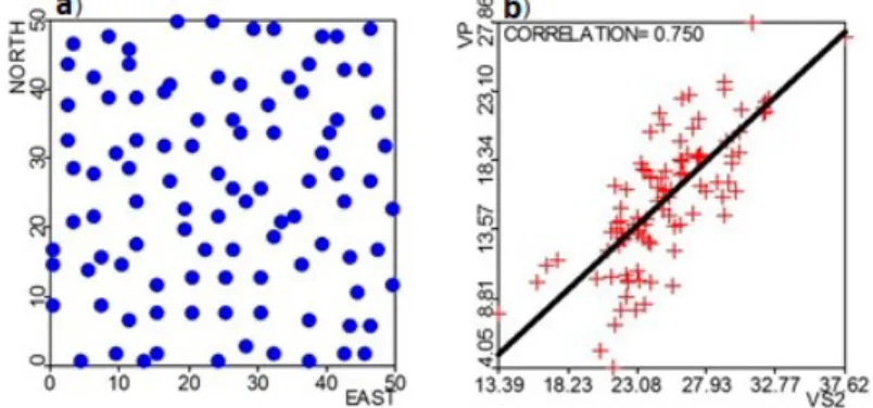
For this study we consider a stratified random sample drawn from an exhaustive data set composed of 2500 data points arranged in an array of 50 rows by 50 columns. This sample, with 100 data points (4% of the exhaustive) presents two measured variables (VP and VS2) in each location (Figure 1a). These variables present a positive correlation (Figure 1b). In addition to performing arithmetic operations between VP and VS2, we have to prove that mean and variances of combined variables are valid. Thus, we generated four new variables: VP+VS2; VP-VS2; VPxVS2 and VP/VS2. Sample statistics for all variables are presented in Table II.
Figure 1 -Location map of sample data (a) and VP X VS2 scattergram (b) (see the colors in the online version).
VP and VS2 will be used for building raster maps, from which we want to obtain new raster maps by combining them arithmetically. Mean and variance for new random variables are listed in Table III. Comparing these results with directly computed statistics in Table II, we verify that except for the quotient of random variables, all others are exactly the same.
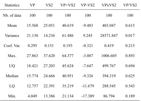
TABLE II
Sample statistics for variables VP, VS2, VP+VS2, VP-VS2, VPxVS2 and VP/VS2.
Statistics VP VS2 VP+VS2 VP-VS2 VPxVS2 VP/VS2
Nb. of data 100 100 100 100 100 100
Mean 15.568 25.051 40.619 -9.483 403.047 0.615 Variance 21.130 14.236 61.486 9.245 28571.847 0.017 Coef. Var. 0.295 0.151 0.193 -0.321 0.419 0.215 Max. 27.863 37.620 64.377 -3.087 1006.605 0.893 UQ 18.421 27.203 45.624 -7.647 499.767 0.694 Median 15.774 24.666 40.951 -9.326 394.319 0.625 LQ 12.757 22.391 35.219 -11.679 288.545 0.543 Min. 4.049 13.386 21.134 -17.389 86.794 0.189 UQ=upper quartile and LQ=lower quartile.
to compute cells of the VP raster maps and equations (25) and (29) for VS2 raster maps. The covariance between VP and VS2 will be calculated after equation (27). These statistics will be combined according to formulas in Table I to derive means and uncertainties of resulting arithmetically combined raster maps. Now, we can compare resulting raster maps with those computed directly from new variables based on equations (16) and (17). Next, these equations ((21) and (23)) will be checked against equations (10) and (11) for variables VP±VS2, equations (12) and (13) for variable VPxVS2 and equations (14), (15), (16) and (17) for variable VP/VS2.
RESULTS AND DISCUSSION
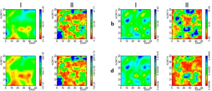
Raster maps for variables VP and VS2 are presented in Figure 2. For the purpose of displaying interpolation variances and covariance, we considered a maximum equal to 95% of their distributions. Now, raster maps for VP and VS2 can be combined by applying arithmetic operators. Before proceeding it is important to show raster maps (Figure 3) computed directly from new variables.
The first operation is the sum: VP+VS2. Results of this operation are presented in Figure 4. The result (Figure 4a) is simply the sum of raster maps (for VP and VS2). The variance of the sum (Figure 4b) is equal to the sum of variances for VP(σ2
x)and VS2(σy2)plus twice the covariance between VP and VS2(σxy). The variance of the sum has great influence of the variable VP and the covariance as well. Results illustrated in Figure 4 are exactly the same as shown in Figure 3a.
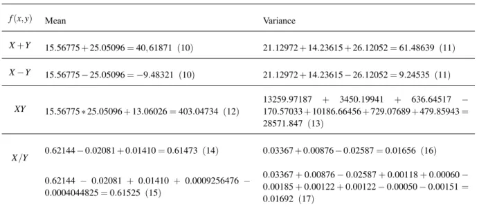
TABLE III
Mean and variance for combined random variables.
f(x,y) Mean Variance
X+Y 15.56775+25.05096=40,61871 (10) 21.12972+14.23615+26.12052=61.48639 (11)
X−Y 15.56775−25.05096=−9.48321 (10) 21.12972+14.23615−26.12052=9.24535 (11)
XY 15.56775∗25.05096+13.06026=403.04734 (12)
13259.97187 + 3450.19941 + 636.64517 −
170.57033+10186.66456+729.07689+479.85943=
28571.847 (13)
X/Y 0.62144−0.02081+0.01410=0.61473 (14) 0.03367+0.00876−0.02587=0.01656 (16)
0.62144 − 0.02081 + 0.01410 + 0.0009256476 −
0.0004044825=0.61525 (15)
0.03367+0.00876−0.02587+0.00118+0.00060−
0.00185+0.00122+0.00122−0.00050−0.00151=
0.01692 (17)
with the variance of VS2 and the covariance. Mean and variances computed after equations (10) and (11) for addition and subtraction match those values computed directly from equations (21) and (23). Once again, results can be compared graphically with images presented in Figure 3b.
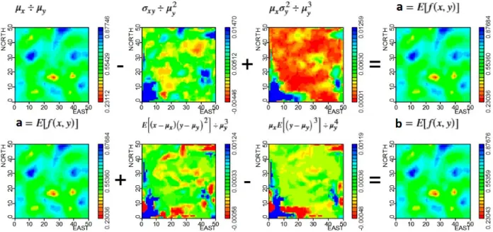
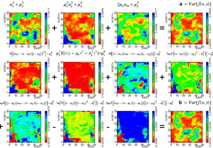
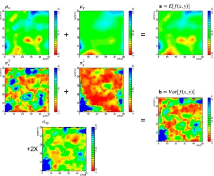
The results of the multiplication of VP and VS2 are presented in Figure 6, which can be compared with results of direct multiquadric interpolation of the variable VPxVS2 (Figure 3c). The mathematical expectation of this operationE[f(x,y)]is equal to the product of VP and VS2 plus the covariance between VP
and VS2. Note that the mathematical expectation has the contribution of the covariance.E[f(x,y)]is highly
correlated with the meansµxandµy and low correlation with the covariance. The uncertaintyVar[f(x,y)] is equal to term 1(µ2
yσx2)plus term 2(µx2σy2)plus term 3(E h
(x−µx)
2
(y−µy)
2i
)minus term 4(σ2
xy)plus term 5(2µxµyσxy)plus term 6
2µyE
h
(x−µx)
2
(y−µy) i
plus term 7 2µxE
h
(x−µx) (y−µy)
2i . Next, the variance was calculated after second-order Taylor expansion (equation (13)) and therefore higher order moments have been included. Equations (12) and (13) provided the same results as applying equations (21) and (23) for the new random variable VPxVS2.
Figure 2 -Raster maps for variables VP (a) and for variable VS2 (b). Interpo-lated variables in column I, uncertainties in column II and covariance between VP and VS2 in column III. Interpolation variances and covariance were dis-played for a maximum equal to 95% of their distributions (for the interpretation of the references to color in this figure legend, the reader is referred to the web version of this article).
Figure 4 -Results of arithmetic operation VP+VS2. The result (a) is equal to the sum of VP(µx)and VS2(µy). The associated uncertainty (b) is equal to the
variance of VP(σ2
x)plus variance of VS2(σy2)plus twice the covariance between VP and VS2 σxy
(for the interpretation of the references to color in this figure legend, the reader is referred to the web version of this article).
Figure 5 -Results of arithmetic operation VP-VS2. The result (a) is equal to the sum of VP(µx)and VS2(µy). The associated uncertainty (b) is equal to the
vari-ance of VP(σ2
x)plus variance of VS2(σ
2
Figure 6 -Results of arithmetic operation VPxVS2. The result(E[f(x,y)])is equal to the product of VP(µx)and VS2 µy plus the covariance between VP and VS2 σxy. The associated uncertainty(Var[f(x,y)])is equal to the term 1(µy2σ
2
x)plus the term 2(µ2
xσy2)plus the term 3(E
h
(x−µx)2 y−µy
2i
)minus the term 4(σ2
a better approach than the equation (14). On the other hand, the variance after equation (17) is much better than that provided by equation (16).
We can follow arithmetic operations taking as an example the cell with coordinates CX=29.50 and CY=23.5 (Table IV). With eight neighbor data we interpolated this cell using field data for VP and VS2. All other variables (VP+VS2, VP-VS2, VPxVS2 and VP/VS2) were derived from these measurements (VP and VS2). Note that we can compute mean and variance directly for derived variables and thus these values can be checked against statistics computed using formulas listed in Table I. In Table IV, the data point with coordinates (CX=26.5, CY=25.5) has a weight equal to zero. This is because we applied an algorithm for correcting negative weights (Rao and Journel 1997), in which a constant equal to the modulus of the largest negative weight was added to all weights and then restandardized to a sum equal to one.
Figure 7 -Mean values for arithmetic operation VP/VS2. (a- upper row) mean after equation (14); (b- lower row) mean according to equation (15) (for the interpretation of the references to color in this figure legend, the reader is referred to the web version of this article).
Mean and variances for the cell with coordinates (CX=29.50, CY=23.5) after combining random vari-ables VP and VS2 are presented in Table V. As can be seen, statistics for VP+VS2, VP-VS2 and VPxVS2 match with statistics computed directly from derived variables listed in Table IV. However, for VP/VS2 we obtain only approximate results.
CONCLUSIONS
Figure 8 -Variances of the arithmetic operation VP/VS2.a) resulting variance from first order Taylor expansion (equation (15));
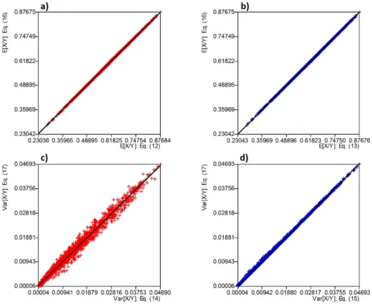
Figure 9 -Scatterplots for means of the ratio of X to Y:a= equation (14) andb= equation (15); variances of the ratio:c= equation (16) andd= equation (17) (see the colors in the online version).
TABLE IV
Neighboring data around a cell with coordinates (CX=29.50, CY=23.5), mean and variances for variables VP, VS2, VP+VS2, VP-VS2, VPxVS2 and VP/VS2.
CX CY W VP VS2 VP+VS2 VP-VS2 VPxVS2 VP/VS2
TABLE V
Mean and variance for combined random variables.
f(x,y) Mean Variance
X+Y 14.57656+24.34917=38.92573 (10) 4.12927+1.65640+2∗0.90406=7.59379 (11)
X−Y 14.57656−24.34917=−9.77261 (10) 4.12927+1.65640−2∗0.90406=3.97755 (11)
XY 14.57656∗24.34927+0.900406=355.83120 (12)
2448.17033 + 351.94621 + 29.44879 −
0.81733 + 641.75335− 473.39666− 95.91113 =
2901.19356 (13)
X/Y
14.57656
24.34917 −
0.90406
(24.34917)2 +
14.57656∗1.65640
(24.34917)3 =
0.59879 (14)
4.12927
(24.34917)2 +
(14.57656)2∗1.65640
(24.34917)4 −
(2∗14.57656)∗0.90406
(24.34917)3 =0.0061402737 (16)
0.0061402737 + 0.0000814529 + 0.0000073085 +
0.0013467544 − 0.0002728552 − 0.0002728552 +
0.0001317723−0.0000235991=0.0071382523 (17)
compute it from a third-order Taylor expansion that provides a slightly better result than the mean computed from second-order Taylor expansion. For the variance of the ratio of X to Y, we demonstrated that the formula based on second-order Taylor expansion provides much better results than the first order.
ACKNOWLEDGMENTS
The authors wish to thank Conselho Nacional de Desenvolvimento Científico e Tecnológico (CNPq) for supporting this research.
REFERENCES
ATKINSON PM AND FOODY GM. 2002. Uncertainty in remote sensing and GIS: fundamentals. In: Foody GM and Atkinson PM (Eds), Uncertainty in Remote Sensing and GIS, p. 1-18.
BURROUGH PA. 1986. Principles of geographical information system. Oxford, Oxford University Press, 194 p.
CROSETTO M, TARANTOLA S AND SALTELI A. 2000. Sensitivity and uncertainty analysis in spatial modelling based on GIS. Agr Ecosyst Environ 81: 71-79.
FRISHMAN F. 1971. On the arithmetic means and variances of products and ratios of random variables. National Technical Information Service, AD-785623, p. 331-345.
HARDY RL. 1971. Multiquadric equations of topography and other irregular surfaces. J Geophys Res 76: 1905-1915. HEUVELINK GB. 1998. Error propagation in environmental modelling with GIS. London, Taylor & Francis, 127 p.
HEUVELINK GB, BURROUGH PA AND STEIN A. 1989. Propagation of errors in spatial modelling with GIS. Int J Geogr Inf Syst 3: 303-322.
JOURNEL AG AND ROSSI M. 1989. When do we need a trend model in kriging? Math Geolo 21: 715-739.
MASKEY S AND GUINOT V. 2003. Improved first-order second moment method for uncertainty estimation in flood forecasting. Hydrolog Sci J 48: 183-196.
MCCALLUM WG. 1998. Multivariable calculus. New York, J Wiley & Sons, 270 p.
MOOD AM, GRAYBILL FA AND BOES DC. 1974. Introduction to the theory of statistics. Tokyo, McGraw Hill, 3rded., 564 p.
WANG G, GERTNER GZ, FANG S AND ANDERSON AB. 2005. A methodology for spatial uncertainty analysis of remote sensing and GIS products Photogramm Eng Rem S 71: 1423-1432.
WEIR MD AND HASS J. 2014. Thomas’ calculus – multivariable. Boston, Person Education Inc, 13thed., p. 572-1044.
WELLMANN FJ, HOROWITZ GF, SCHILL EAND REGENAUER-LIEB K. 2010. Towards incorporating uncertainty of structural data in 3D geological inversion. Tectonophysics 490: 141-152.
YAMAMOTO JK. 2000. An alternative measure of the reliability of ordinary kriging estimates. Math Geol 32: 489-509. YAMAMOTO JK. 2002. Ore reserve estimation using radial basis functions. Rev Inst Geol 23: 25-38.
YAMAMOTO JK, MAO XM, KOIKE K, CROSTA AP, LANDIM PMB, HU HZ, WANG CY AND YAO LQ. 2012. Mapping an uncertainty zone between interpolated types of a categorical variable. Comput Geosci 40: 146-152.
APPENDIX
A1 - MEAN AND VARIANCE OF THE FUNCTIONf(x,y)USING TAYLOR EXPANSION
In this appendix, we develop equations for mean and variance of the functionf(x,y)as presented in Table I.
We will use Taylor expansion of f(x,y)to find the mean and variance of this function around mean values
µx andµy. Besides mean values, variances of random variables (σx2 andσy2)and the covariance between random variables X and Y(σxy)must be known. The development for the mean and variance of product and quotient of random variables was based on Taylor expansion, according to Mood et al. (1974).
According to Weir and Hass (2014), the general equation of Taylor’s Formula for two variables at the pointθ = (a,b)is:
f(x,y) =f(θ) +
h∂f(θ)
∂x +k
∂f(θ)
∂y
+ n
∑
i=2
1
n!
h∂
∂x+k
∂f
∂y
i
f
(θ)
+ 1
(n+1)!
h∂
∂x+k
∂f
∂y
n+1
f
(a+ch,b+ck)
(A1.1)
Whereh= (x−a),k= (y−b),0<c<1and the last term is the remainder. Neglecting the remainder term and taking n=2, we have:
f(x,y) =f(a,b) +∂f(a,b)
∂x (x−a) +
∂f(a,b)
∂y (y−b)
+ 1
2!
∂2
f(a,b)
∂x2 (x−a) 2
+2∂
2
f(a,b)
∂x∂y (x−a) (y−b) +
∂2
f(a,b)
∂y2 (y−b)
2 (A1.2)
Letting(a,b) = (µx,µy)in equation A1.2 we have:
f(x,y) =f µx,µy+fx µx,µy(x−µx) +fy µx,µy y−µy + 1
2!
fxx µx,µy(x−µx)2+2fxy µx,µy(x−µx) y−µy+fyy µx,µy y−µy
2
(A1.3)
Applying the expectation operator to expression A1.3:
E[f(x,y)] =E
f µx,µy+Efx µx,µy(x−µx)+Efy µx,µy y−µy + 1
2!
Ehfxx µx,µy(x−µx)2
i
+2E
fxy µx,µy(x−µx) y−µy+E
h
fyy µx,µy y−µy
Finally:
E[f(x,y)] =f µx,µy+
1 2
σx2fxx µx,µy+2σxyfxy µx,µy+σy2fyy µx,µy
(A1.4)
This is the general expression for mathematical expectation of f(x,y). The variance of the function
f(x,y)can be written as:
Var(f(x,y)) =E. (A1.5)
Replacing A1.2 and A1.3 in A1.4, we get:
Var(f(x,y)) =E. (A1.6)
Calculation of mean and variance for sum and subtraction of random variables X and Y
For f(x,y) =x±y, we have the following derivatives:
fx(x,y) =1
fy(x,y) =±1
fxx(x,y) =0
fxy(x,y) =0
fyy(x,y) =0
Applying them on equations A1.4 and A1.6, we have equations (10) and (11) of Table I:
E[f(x,y)] = f µx,µy
E[f(x,y)] =µx±µy (A1.7)
Var(f(x,y)) =Eh (x−µx)± y−µy
2i
Var(f(x,y)) =Eh(x−µx)2±2(x−µx) y−µy+ y−µy
2i
Var(f(x,y)) =σx2+σ
2
Calculation of the mean and variance for the product of random variables X and Y For f(x,y) =xy, we have the following derivatives:
fx(x,y) =y
fy(x,y) =x
fxx(x,y) =0
fyy(x,y) =0
fxy(x,y) =1
Applying them on equation A1.4, we get equation ((12) - Table I):
E[f(x,y)] =µxµy+σxy (A1.9)
Replacing derivatives in equation A1.6, we have:
Var(f(x,y)) =E
(
µy(x−µx) +µx y−µy
+ (x−µx) y−µy
−σxy
2)
(A1.10)
Notice that:
(a+b+c+d)2=a2+b2+c2+d2+2ab+2ac+2ad+2bc+2bd+2cd (A1.11)
Expanding A1.10 according to A1.11 we obtain:
Var(f(x,y)) =E.
Applying definitions of variance, covariance and the general equation of variance A1.6, we get equation ((13) - Table I):
Var(f(x,y)) =µy2σ
2
x+µ
2
xσ
2
y+2µxµyσxy+E
h
(x−µx)2 y−µy
2i
− σxy
2
+2µyE
h
(x−µx)2 y−µy
i
+2µxE
h
(x−µx) y−µy
2i
(A1.12)
Calculation of the mean and variance for the ratio of X to Y
For calculation of the mean of the quotient of random variables X and Y we will consider second and third order Taylor expansion as follows.
For function f(x,y) =x/y, we have the following derivatives:
fx=1y
fy=−y2x
→ fxx=0
fxy= −y21
fyy=2y3x
→
fxxx=0
fxxy=0
fxyy= y23
Second order Taylor expansion for calculation of the mean of function f(x,y) =x/y:
Applying the derivatives (until second order) on the equation A1.4 we get (equation (14) - Table I):
E[f(x,y)] =µx
µy −σ2
xy
1
µ2
y +σ2
y
µx
µ3
y
(A1.13)
Third order Taylor expansion for calculation of the mean of function f(x,y) =x/y:
Developing equation A1.1 for n=3, we get:
f(x,y) =f(a,b) +∂f(a,b)
∂x (x−a) +
∂f(a,b)
∂y (y−b)
+ 1
2!
∂2
f(a,b)
∂x2 (x−a) 2
+2∂
2
f(a,b)
∂x∂y (x−a) (y−b) +
∂2
f(a,b)
∂y2 (y−b) 2
+ 1
3!
∂3
f(a,b)
∂x3 (x−a) 3
+3∂
3
f(a,b)
∂x2∂y (x−a) 2
(y−b) +3∂
3
f(a,b)
∂x∂y2 (x−a) (y−b) 2
+∂
3
f(a,b)
∂y3 (y−b) 3
(A1.14)
Letting(a,b) = (µx,µy)in equation A1.14, we have:
f(x,y) =f(µx,µy) +fx(µx,µy)(x−µx) +fy(µx,µy)(y−µy) + 1
2!(fxx(µx,µy)(x−µx)
2
+2fxy(µx,µy)(x−µx)(y−µy) +fyy(µx,µy)(y−µy)2)
+ 1
3!(fxxx(µx,µy)(x−µx)3+3fxxy(µx,µy)(x−µx)2(y−µy) +3fxyy(µx,µy)(x−µx)(y−µy)
2
+fyyy(y−µy)3) (A1.15)
Replacing derivatives in equation A1.15 we have (equation (15) - Table I):
E[f(x,y)] = µx
µy −σxy
1
µ2
y +σy2
µx
µ3
y +
Eh(x−µx) y−µy
2i
µ3
y
−µx
µ4
y
Eh y−µy
3i
(A1.16)
First order Taylor expansion for calculation of the variance of function f(x,y) =x/y:
To obtain the expression for variance using First order Taylor expansion, we will develop the equation A1.1 without the summatory term, then we have:
f(x,y) =f(a,b) +∂f(a,b)
∂x (x−a) +
∂f(a,b)
∂y (y−b) (A1.17)
Letting(a,b) = (µx,µy), we have:
f(x,y) =f µx,µy
+fx µx,µy
(x−µx) +fy µx,µy
y−µy
E[f(x,y)] =f µx,µy
And for the variance:
Var(f(x,y)) =Eh fx µx,µy(x−µx) +fy µx,µy y−µy
2i
Var(f(x,y)) =E
h
fx2 µx,µy
(x−µx)2+2fx µx,µy
fy µx,µy
(x−µx) y−µy
+fy2 µx,µy
y−µy
2i
Applying the corresponding derivatives (until first order) we get (equation (16) - Table I):
Var(f(x,y)) =σ
2
x
µ2
y −2µx
µ3σxy+ µ2
x
µ4
y
σy2 (A1.18)
Second order Taylor expansion for calculation of the variance of function f(x,y) =x/y(equation A1.6):
Var(f(x,y)) =E
("
1
µy
(x−µx)−µx
µ2
y
y−µy −1
µ2
y
(x−µx) y−µy−σxy+
µx
µ3
y
h
y−µy
2
−σy2
i #2
Var(f(x,y)) =E
("
(x−µx)
µy −µx
µ2
y
y−µy +
σxy−(x−µx) y−µy
µ2
y
+ µx
µ3
y
h
y−µy
2
−σ2
y i #2 (A1.19)
Expanding A1.19 according to A1.11 we obtain:
Var(f(x,y)) =E. (A1.20)
Developing and simplifying, we get equation ((17) - Table I):
Var[f(x,y)]≈σ
2 x µ2 y +µ 2 x µ4 y
σy2−2
µx
µ3
y
σxy+
1
µ4
y
Eh σxy−(x−µx) y−µy
2i +µ 2 x µ6 y E
y−µy
2
−σy2
2
+ 2
µ3
y E
(x−µx)
σxy−(x−µx) y−µy+2
µx
µ4
y
Eh(x−µx)h y−µy
2
−σy2
ii
−2µx
µ4
y E
y−µy σxy−(x−µx) y−µy−2
µ2 x µ5 y E h
y−µy
h
y−µy
2
−σy2
ii
+2µx
µ5
y Eh
σxy−(x−µx) y−µy
h
y−µy
2
−σ2
y
ii
(A1.21)
A2 - HEUVELINK’S APPROACH FOR CALCULATION OF THE MEAN AND VARIANCE OF FUNCTIONf(x,y)BASED ON SECOND ORDER TAYLOR EXPANSION
In this appendix we wanted to show that the traditional approach used in Appendix A1 gives the same results as obtained by Heuvelink et al. (1989) and Heuvelink (1998). Actually, these references presented a general formula of second order Taylor expansion for n random variables.
The second order Taylor expansion of a function with n variables at the point M=(µ1,...,µn) and
f(x´) =f(M) + n
∑
i=1
[(xi−µi)fxi(M)] +
1 2
n
∑
i=1
n
∑
j=1
(xi−µi) xj−µjfxixj(M)
(A2.1)
Then, the mean around M is computed as (Heuvelink 1989):
E(f(M)) =E[f(M)] +E
"n
∑
i=1
[(xi−µi)fi(M)]
# +1 2E "n
∑
i=1 n∑
j=1(xi−µi) xj−µjfij(M)
#
E(f(M)) =f(M) +1
2
n
∑
i=1
n
∑
j=1
ρijσiσjfij(M) (A2.2)
Whereρijis the correlation coefficient between variablesiandj;σiis the standard deviation for variable
iandσj is the standard deviation for variable j.
Var(x´) =E
" n
∑
k=1[(xk−µk)fk(M)] +
1 2 n
∑
i=1 n∑
j=1(xi−µi) xj−µj
−ρijσiσj
fij(M)
#2
Var(x´) = n
∑
k=1 n∑
l=1ρklσkσlfk(M)fl(M)
+ n
∑
k=1 n∑
i=1 n∑
j=1E(xk−µk) (xi−µi) xj−µj
−ρklσkσl
fk(M)fij(M)
+?1 4 n
∑
i=1 n∑
j=1 n∑
k=1 n∑
l=1E(xi−µi) xj−µj
(xk−µk) (xl−µl)−ρijσiσjρklσkσl
∗?∗fij(M)fkl(M)
(A2.3)
Notice that for n=2, and setting x1=x and x2=y, the expression A2.2 becomes:
E(f(x,y)) =f µx,µy+
1 2
σ2
xfxx µx,µy+2σxyfxy µx,µy+σy2fyy µx,µy
(A2.4)
Expressions A1.3 and A2.4 are the same, so the development of the expectation for an arithmetic opera-tion is the same as shown in Appendix A1. Therefore, equaopera-tions (10), (12) and (14) of Table I can be derived from A2.4.
For the variance, we will need to expand the expression A2.3 and consider the arithmetic operation regarding the function f(x,y). Then at the pointµ= (µx,µy)we have:
Var(x,y) =σ2
xfx2(µ) +2σxyfx(µ)fy(µ) +σy2fy2(µ) +Eh(x−µx)3−(x−µx)σx2
i
fx(µ)fxx(µ) +2Eh(x−µx)2 y−µy−(x−µx)σxy
i
fx(µ)fxy(µ) +Eh(x−µx) y−µy
2
−(x−µx)σ2
y
i
fx(µ)fyy(µ) +E
h
(x−µx)2 y−µy
− y−µy
σ2
x
i
fy(µ)fxx(µ) +2E
h
(x−µx) y−µy
2
− y−µy
σxy
i
fy(µ)fxy(µ)
+Eh y−µy
3
− y−µy
σ2
y
i
fy(µ)fyy(µ) +
1
Calculation of the variance for sum and subtraction of random variables X and Y
Since for f(x,y) =x±yall second order derivatives are equal to zero, we have (equation (11) - Table I):
Var(x,y) =σ2
x+σ
2
y±2σxy (A2.5)
Because all second order derivatives are equal to zero.
Calculation of the variance for the product of random variables X and Y
Var(x,y) =σx2µ
2
y+σ
2
yµ
2
x+2σxyµxµy+2µyE
h
(x−µx)2 y−µy
i
+2µxE
h
(x−µx) y−µy
2i
+Eh(x−µx)2 y−µy
2i
− σxy
2
(A2.6)
This is the same as equation ((13) - Table I).
Calculation of the variance for the ratio of X to Y
Var(x,y) =σ
2
x
µ2
y −2µx
µ3
y
σxy+
µ2 x µ4 y σ2 y− 2 µ3 y
Eh(x−µx)2 y−µy−(x−µx)σxy
i
+2µx
µ4
y
Eh(x−µx) y−µy
2
−(x−µx)σ2
y
i
+2µx
µ4
y
Eh(x−µx) y−µy
2
− y−µyσxy
i
−2µ
2
x
µ5
y
Eh y−µy
3
− y−µyσy2
i
+1
4
(
−42µx
µ5
y
Eh(x−µx) y−µy
3
−σ2
yσxy
i
+4 1
µ4
y
Eh(x−µx)2 y−µy
2
− σxy
2i
+ 4µ
2 x µ6 y E
y−µy
4
−σ2
y
2)
Var(x,y) =σ
2 x µ2 y +µ 2 x µ4 y
σy2−2
µx
µ3
y
σxy+
2
µ3
y E
(x−µx)
σxy−(x−µx) y−µy
+2µx
µ4
y
Eh(x−µx)h y−µy
2
−σ2
y
ii
−2µx
µ4
y E
y−µy σxy−(x−µx) y−µy
−2µ
2
x
µ5
y
Eh y−µy
h
y−µy
2
−σ2
y
ii
−2µx
µ5
y
Eh(x−µx) y−µy
3
−σ2
yσxy
i
+ E
h
(x−µx)2 y−µy
2i
− σxy
2 µ4 y +µ 2 x µ6 y E
y−µy
4
−σy2
2
(A2.7)
As we can see, some terms of equation A2.7 do not match A1.21. Actually, we can rewrite these terms as follows.
Eh
σxy−(x−µx) y−µy
2i
= σxy
2
−2σxyE(x−µx) y−µy+E
h
(x−µx)2 y−µy
2i
=Eh(x−µx)2 y−µy
2i
− σxy
2
E
h
y−µy
2
−σ2
y
i2
=E
h
y−µy
4i
−2σ2
yE
h
y−µy
2i
+σ2
y
2
=E
h
y−µy
4i
−σ2
y
2
=E
y−µy
4
−σ2
y
E
h
σxy−(x−µx) y−µy
h
y−µy
2
−σy2
ii
=E
h
(x−µx) y−µy
−σxy
h
σy2− y−µy
2ii
=Eh(x−µx) y−µyσy2
i
−Eh(x−µx) y−µy
3i
−Ehσxyσy2
i
+Ehσxy y−µy
2i
=Ehσxyσy2
i
−Eh(x−µx) y−µy
3i
=Ehσxyσy2−(x−µx) y−µy
3i
![Figure 6 - Results of arithmetic operation VPxVS2. The result (E [f (x,y)]) is equal to the product of VP (µ x ) and VS2 µ y plus the covariance between VP and VS2 σ xy](https://thumb-eu.123doks.com/thumbv2/123dok_br/16000993.691488/12.892.76.768.247.830/figure-results-arithmetic-operation-vpxvs-result-product-covariance.webp)