A NALYSIS OF POVERTY AND SOCIAL EXCLUSION WITH PANEL

M

ASTER

A

PPLIED

E

CONOMETRICS AND

F

ORECASTING

M

ASTER

´

S

F

INAL

W

ORK

D

ISSERTATION

A

NALYSIS OF POVERTY AND SOCIAL EXCLUSION WITH PANEL

MICRODATA

J

OSÉ

M

IGUEL

R

AMOS

M

ODESTO

A

PPLIED

E

CONOMETRICS AND

F

ORECASTING

M

ASTER

´

S

F

INAL

W

ORK

D

ISSERTATION

ANALYSIS

OF

POVERTY

AND

SOCIAL

EXCLUSION

WITH

PANEL

MICRODATA

J

OSÉ

M

IGUEL

R

AMOS

M

ODESTO

SUPERVISION:

I

M

D

P

A

C

M

A

B

I

Acknowledges

I would like to thank, personally, to Professor Isabel Proença and to Professor Amélia Bastos, for all the support and knowledge they provided to the successful conduction of this dissertation. I wish both much happiness and success on future investigations!

I would like to also thank my girlfriend, Ana Isabel Boleto, and both my father and my mother, in all the support and conditions they provided for me, to reach my goals.

A sincere Thank You, to all of You!

II

Abstract

This dissertation intends to model the dynamics of social exclusion by investigating the individual characteristics that contributes to increase the probability of being socially excluded, as well as the identification of the most vulnerable population groups.

We will be using the criteria proposed by the Eurostat to define social exclusion, and we will be using a four years longitudinal data from European Statistics on Income and Living Conditions relative to the Portuguese population. We aggregate the criteria into a binary indicator of social exclusion, so we will be applying a Pooled Probit and a Random Effects Probit model to the data.

This work also intends to enrich the literature about this subject, as we were able to reach interesting results, relative to the determinants of social exclusion and some of the most vulnerable groups to this phenomenon.

Keywords: Social Exclusion, Panel Data, Probit, Poverty, Material Deprivation,

III

Resumo

Esta dissertação propõe-se a modelar a dinâmica da exclusão social ao investigar as características dos indivíduos que contribuem para aumentar a probabilidade deste se encontrar em situação de exclusão social, assim como identificar os grupos mais vulneráveis.

Para o efeito, vamos usar o critério proposto pelo Eurostat para definir a exclusão social, usando uma base de dados longitudinal de quatro anos do ICOR (Inquérito para as Condições de Vida e Rendimento) relativa à população portuguesa. O critério é traduzido num indicador binário de exclusão social, assim sendo, recorremos aos modelos Pooled Probit e Probit de Efeitos Aleatórios para modelar os nossos dados.

Este trabalho tem também como objetivo enriquecer a literatura existente acerca desta matéria, e possibilitou-nos alcançar resultados interessantes, relativos às características que ajudam a explicar a probabilidade de ocorrência de exclusão social e aos grupos que se mostram mais vulneráveis a este problema.

Palavras-chave: Exclusão Social, Dados em Painel, Probit, Pobreza, Privação

Material, Baixa Intensidade Laboral, Desemprego, Vulnerabilidade, Desvantagens

IV

Table of Contents

I. INTRODUCTION ... 1

II. BACKGROUND ... 2

I. DEFINITION OF SOCIAL EXCLUSION ... 2

II. ECONOMETRIC APPROACHES ... 3

III. DATA ... 7

IV. METHODOLOGY ... 11

V. EMPIRICAL RESULTS ... 17

VI. CONCLUSION ... 21

REFERENCES ... 23

APPENDIX 1 – TABLES ... 25

1

I.

Introduction

Social exclusion represents a major challenge in todays’ society. It can prevent the

individual from participate in many aspects of life in society, degrading life expectations, social cohesion, and thus, decreasing the sense of belonging to the community and compromising economic prosperity. Measuring social exclusion is also a challenge, since it can be describe as a multidimensional and dynamic process, and there is no consensus on a formal threshold. This work will present some of the different definitions adopted by several investigators, but will formally stand for the Eurostat definition when analysing the data and applying an econometric model to it. Econometric methods have been popular in conducting studies on social exclusion, due to the robustness and consistency of its results, as well as its success in translating the dynamics towards the process of social exclusion.

This works aims to contribute to a more enlightment about the social exclusion reality, its determinants, who are the most vulnerable and seeks to explain which variables contribute to a higher propensity of experiencing social exclusion. The higher concern about this subject is motivated by the Europe 2020 strategy, which propose to diminish the number of European Union citizens socially excluded by 20 million, strengthening the European society for the challenges of the next decades. Schienstock et al. (1999) explores the challenges brought by the new social structures of the Information Society, one of them being the risk of increasing the prevalence of social exclusion among population.

2

II.

Background

Several authors have been paying attention to social exclusion for the past few years, due to the challenges that it generates to society and public decisors. At this point, we see the necessity to explore some studies that have been made within this subject, to briefly summarize the main conclusions.

i.

Definition of Social Exclusion

Contrarily to other social issues, such as poverty, it has not been identified a formal social exclusion threshold (Silver, 2007). Moreover, different authors frequently presents different definitions. Poggi (2003), stating Lee-Murie (1999), defines social exclusion as a process that excludes individuals from social, economic and cultural networks, and which has been linked to the idea of citizenship. Silver (2007) gives a more precise definition, defining social exclusion as a rupture of social relations, institutions, social cohesion, integration or solidarity. Tsakloglou and Papadopoulos (2002) stating Silver (1994), de Haan (1998) and Byrne (1999), says that social excluded individuals are those unable to exercise social, political and civil rights or to participate on a diversity aspects of life in society. Additionally, stating Mayes et al. (2001) and Atkinson et al. (2002), they also interpret social exclusion as exclusion from the labour market and material deprivation. In the same article they suggest social exclusion to be a chronic cumulative disadvantage. According to D’Ambrosio and Chakravarty (2003), the European Commission’s Programme specification for ‘targeted socioeconomic research’ defines

3

process leading to cumulative disadvantages of various forms. These are just some examples of the diversity of suggestions for the definition of social exclusion.

A conclusion we can extract from these, and which is frequently mentioned among researchers, is that social exclusion is a multidimensional and dynamic process. Therefore, longitudinal data are the most widely used to investigate this phenomenon.

For quantitative purposes of this work, we will consider an individual as social excluded using the Eurostat criteria, which is standing for at least one of the following three dimensions: at risk of poverty1, material deprivation2, or living in a household with a very low work intensity3.

ii.

Econometric approaches

Many approaches were followed by many authors for them to reach their conclusions, and many were the aspects considered. Poggi (2007) states that we can have true state of dependence (where the probability of being socially excluded in the future depends of whether or not the individual already experienced it in the past), observed characteristics (such as scholarship, gender, parenthood, and others) and unobserved heterogeneity (the characteristics which can not be observed or measured and are inherent to the individual, i.e., are constant in time). Poggi estimates a dynamic random effects logit model with both lagged dependent and exogenous variable, in which the dependent variable is an indicator that can assume the value of one if exclusion occurs, and zero

1 _{A person is said to be at risk of poverty if he or she is below the at-risk-of-poverty threshold, which is}

set at 60 % of the median income per adult equivalent after social transfers

2 _{A person is said to be materially deprived if he or she can not afford at least three out of a list of nine}

items established by the social protection committee

3 _{A household with very low work intensity is defined as a household where the members worked less}

4

otherwise. Another methodological aspect is that Poggi considers an individual as being excluded if the individual is, at least, excluded in one dimension among eight4. Some of the author’s main conclusions is the strong presence of a true state dependence, that being

lone parent or less educated seems to raise significantly the probability of being socially excluded, and that the region where the individual lives also appears to be important to explain social exclusion. Another interesting idea is that social exclusion, through the introduction of year dummies, seems to decrease over time.

Tsakloglou and Papadopoulos (2002) have an interesting suggestion, analysing the high risk of social exclusion trough several European countries, and highlighting the differences among them. For usage in statistic (and econometrics) aspects, they consider at high risk of social exclusion those who are deprived in at least two, among four, deprivation indicators, being these lack of income (also known as poverty), living conditions, necessities of living, and social relations. One interesting result, is that we can find higher rates of population in high risk of social exclusion in poorer countries according to the first three criteria, but not to the fourth. They also look for individual characteristics that may help explain the probability of being in high risk of social exclusion. One interesting idea, is besides measuring for the individual self-characteristics, they go for the characteristics of the reference person of the individual’s

household. They do this using a logistic regression, and find that the ‘effects associated

with educational qualifications of the household’s reference person are stronger than those associated with the educational qualifications of the individual’. Other results shows

that lack of full-employment, low educational qualifications, lone parenthood, non-EU

4These dimensions are “the basic need fulfilment”, “living in a safe and clean environment”, “having an

5

citizenship and bad health are associated with increased risk of social exclusion, and qualifying countries in groups according to their type of welfare regime allows to see here statistical significance also. It was even possible to conclude that in several ways, the country where the individual is from, impacts the probability of being at high risk of social exclusion due to a specific individual characteristic. For example, elderly people have an increased high risk of social exclusion in some southern countries, but a reduced risk in some northern countries. This results advice for, being the reality among European countries very different, the problem of social exclusion shall have different approaches. All the previous authors talked about and showed results estimated for lone parenthood. Heavily related to social exclusion is early motherhood as well, and Hobcraft and Kiernan (2001) explored deeply the questions associated to this phenomenon. They divided a population of women in four categories, those who were mothers for the first time under age 20, between 20 and 22, 23 to 32 and those who were not mothers at age 33. In a first stage, they control for eleven variables representing different outcomes in adult life (such as ill-health and social housing), and found high correlation between all these variables and early motherhood. After that, they tested for child poverty (and other factors, such as contact with police by age 16), and to do so, they applied a logistic regression. One of the main conclusions, is that adverse adult outcomes are more significantly more probable to occur for those who enter motherhood early, and that having experienced child poverty increases the chances of becoming an early mother. One interesting idea is that this can also suggest the concept of true state of dependence. Thus, poverty has been closely linked to social exclusion several times. Bradshaw et al.

6

7

unemployed in specific social environments. On the second phase, they find that the unemployed who were poor took significantly more time to exit unemployment. So the main conclusion is the existence of a vicious circle between poverty and unemployment, with very little relation to social exclusion.

III.

Data

As previously presented, in this work we are looking to explain social exclusion through individuals’ and households’ characteristics, investigating who are the most vulnerable groups, and analysing which characteristics contributes to that vulnerability.

We will be using longitudinal data from European Statistics on Income and Living Conditions, for the population living in the Portuguese territory, from years 2010 to 2013. This includes a diversity of information such as income, housing conditions, scholarship, presence in labour market, health, and so on.

8

information are mainly elderly or people with very low scholarship, who had some difficulty on completing the inquiry. This definitely represents a limitation on our analysis.

9

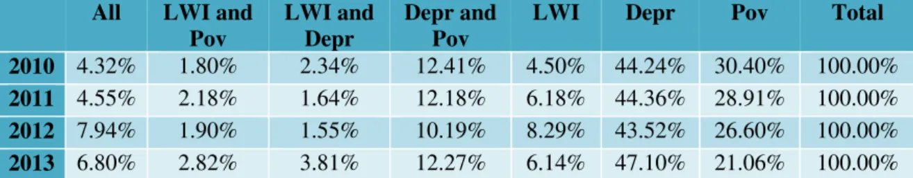
In fact, when looking at table IX Appendix I, the median income in our sample decreases 2.82% from 2010 to 2013. Another reasonable explanation, is that some people that were at risk of poverty alone on the beginning of the period in analysis, later on started to experiencing also one, or both, of the other two dimensions; table VII Appendix I shows us that people living in a household with very low work intensity and at risk of poverty increased, and people experiencing all three dimensions had a more significant increase. This also tell us that not only have social exclusion increased, its severity has also increased.

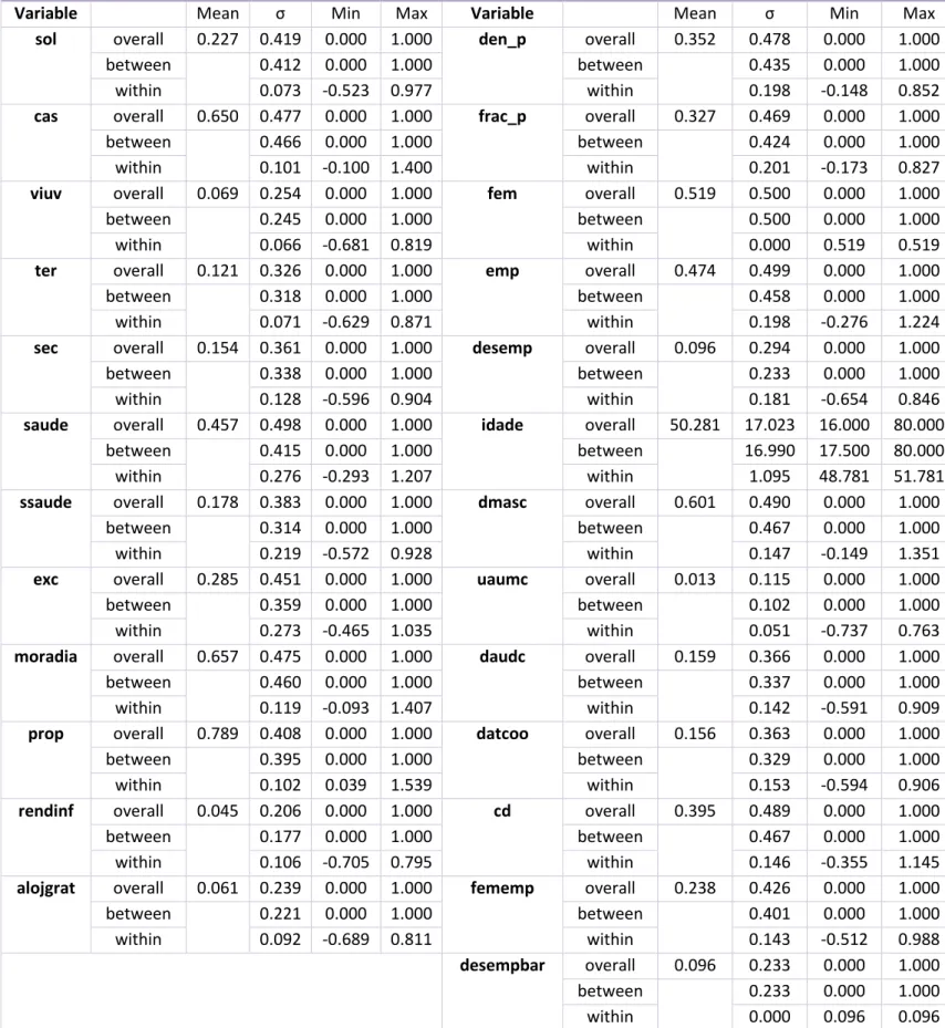
On table V Appendix I we can see the description for each variable we tested. The meaning of each variable is as follows: exc– our dependent variable, a dummy variable with value one if the individual is socially excluded according to the indicator we adopted, and zero otherwise; sol, cas, and viuv– dummy variables, with sol assuming value one if the individual is single and zero otherwise, cas assuming value one if the individual is married and zero otherwise, and viuv assuming value one if the individual is a widow or a widower (being the divorced and separated the reference group); ter and sec– dummy variables, with ter assuming value one if the individual has tertiary education and zero otherwise, and sec assuming value one if the individual has secondary education and zero otherwise (being the reference group those that have less than secondary education);

saude and ssaude – dummy variables, with saude assuming value one if the individual considers his or her health status good or very good and zero otherwise and ssaude

10

alojgrat and rendinf– dummy variables, with prop assuming value one if the individual (or another member of the household) owns the residence in which he or she lives and zero otherwise, alojgrat assuming value one if the individual lives in an accommodation provided by someone else without any costs or provided by in exchange for a wage and zero otherwise, and rendinf assuming value one if the individual lives in a rented house with a supported rent (being the tenants without any supports the reference group); den_p

and frac_p– dummy variables, with den_p assuming value one if the individual lives in a high density populated area and zero otherwise, and frac_p if the individual lives in a low density populated area (being those who live in a fair density populated area the reference group); fem– dummy variable with value one if the individual is a female and zero otherwise (males are the reference group); fememp– dummy variable with value one if the individual is an employed female and zero otherwise (being the reference group those who are male or unemployed or inactive female); emp and desemp – dummy variables, with emp assuming value one if the individual is employed and zero otherwise, and desemp assuming value one if the individual is unemployed and zero otherwise (being those who are inactive the reference group); idade – gives the age of the individual;

dmasc, uaumc, daudc and datcoo– dummy variables, with dmasc assuming value one if the individual lives in a household with two or more adults without children and zero otherwise, uaumc assuming value one if the individual lives in a household with one adult and one or more children and zero otherwise, daudc assuming value one if the individual lives in a household with two adults and one or two children and zero otherwise, and

11

dummy variable with value one if the individual lives in a household with dependent children5, and zero otherwise (being the individuals who lives in a household without dependent children the reference group).

The reason why we considered the employed females (fememp) is because, as we will see further, the female (fem) alone proved to not to be statistical significant, and we decided to search deeper for any evidence of gender inequality there might be, since it is well known the disadvantages that women can still face in work places nowadays, more than in general society. Matter of fact, the variable fememp showed to be statistical significant. We will have the opportunity to explore and discuss more the context and findings related to this later on.

For each of these variables, we can descriptive statistics on table IV Appendix I.

IV.

Methodology

In this chapter we aim to describe the methodology adopted to reach our results. As mentioned before, several approaches were used in the past to study social exclusion, the phenomenon and the process itself, its implications as well the reality and the conditions that stimulate its growth. Tsakloglou and Papadopoulos (2002) presented results for the interesting idea that the determinants of social exclusion can vary between different countries in the European Union, which is a reasonable idea when we think of the importance of the family structure, the social relationships and the strength of the social institutions and politics, which can vary deeply between different cultures. In this paper

5 _{The diference between children and dependent children, according to the Eurostat criteria, is that}

12

we aim to explain the probability of experiencing social exclusion throughout the self-characteristics of the individuals in the Portuguese reality, on an attempt to reveal who are the most vulnerable groups.

Now, remember that social exclusion is not a binary concept, but instead a dynamic process that leads the individual to not participate in the society in many different ways and in many different levels, existing a combination of social forces, contributing to integrate the individual among us, or contributing to marginalize. Said this, we cannot measure how much an individual participate in society, but instead we observe if he or she is socially excluded according to the Eurostat criteria.

So, consider the following latent, not observed, variable model:

(1) y∗ = (social forces marginalizing) − (social forces integrating) = (x γ + ε1) − (x δ + ε2) = x β + ε

Where x = (x₁, x₂, … , x_p) is the vector of regressors, β′= (β₁, β₂, … , β_p) the vector of coefficients, and y∗ is the level of participation in society.

And being y the binary indicator following Eurostat criteria such that: (2) y = { 1, y

∗ _{> 0}

0, otherwise

We are interesting in estimate the probability of an individual to be socially excluded according to the indicator we are following, so we can state:

(3) P(y = 1|x) = P(y∗ > 0|x) = P(xβ + ε > 0|x) = P(ε > −xβ|x) = P(ε < xβ|x) = G(xβ)

13

since we are considering the Probit model, we will specify a normal distributed form, i.e., ε|x ~ N(0,1) and equation (3) become

(4) P(y = 1|x) = Φ(xβ)

We will be using panel data, as it gives a richer analysis, so therefore, the models to be considered are the random effects Probit and the pooled Probit.

The random effects Probit can be written in the form:

(5) P(y_it = 1|x_it, 𝑐_𝑖) = 𝛷(x_itβ + c_i), t = 1, … , T; i = 1, … , N

Where x_it = (x_it,1, x_it,2, … , x_it,p) is the vector of regressors, β′= (β₁, β₂, … , β_p) the vector of coefficients and c_i being the individual unobserved heterogeneity. Unobserved heterogeneity are the characteristics inherent to the individual and constant in time, that we do not observe and that are correlated with the other variables. Since it is a relevant information that keeps omitted, the other variables present in the model becomes correlated with the error term. This is known as endogeneity and it is a violation of a basic assumption of the model, causing it to be biased.

Obviously, since we are considering more information than we do on the pooled Probit model (which ignores the unobserved heterogeneity), we can make more efficient estimations. Unfortunately, this comes with a cost. Random effects Probit model is only consistent when we specify the true density of the function, and it assumes that ci|xi~Normal(0, σc2), which is a very strong assumption, since it implies that ci has a

14

we need to estimate β_c = β/(1 + σ_c2)1/2. This can be done by maximizing the log-likelihood function, which can be written as:

(6) lnL(β, σc) = ∑ ln N

i=1

(∫[ ∏ 𝛷

T

t=1

(xitβ + ci)yit[1 − 𝛷(xitβ + ci)]1−yit](1 σ⁄ )𝜙(cc i⁄ )dcσc i)

And the average partial effects for a dummy xtk is 𝑛−1∑ {𝛷[𝑛_𝑖=1 𝛽₁𝑥_𝑖1+ 𝛽₂𝑥_𝑖2+

⋯ + 𝛽𝑘−1𝑥𝑖𝑘−1+ 𝛽𝑘(1)] − 𝛷[𝛽1𝑥𝑖1+ 𝛽2𝑥𝑖2+ ⋯ + 𝛽𝑘−1𝑥𝑖𝑘−1+ 𝛽𝑘(0)]}.

The alternative to this model leads us to the pooled Probit model. It can be written in the form:

(7) P(y_it = 1|x_it) = 𝛷(x_itβ), 𝑡 = 1, … , T; i = 1, … , N

Again, x_it = (x_it,1, x_it,2, … , x_it,p) is the vector of regressors and β′= (β₁, β₂, … , β_p) the vector of coefficients. A consistent estimator of β can be obtained by maximizing the

partial log-likelihood function, which can be written as:

(8) ∑ ∑ [yN_i=1 T_{t=1 it}ln𝛷(x_itβ) + (1 − y_it) ln[1 − 𝛷(x_itβ)]]

The pooled Probit estimator considers N independent observations, allowing for dependency on time. Furthermore, it only requires contemporary exogeneity, making it a more robust estimator than the random effects Probit, although less efficient.

When applying the pooled Probit estimator, it is recommended to use a cluster robust variance matrix (whose the cluster is the individual) to control for conditional correlation between y_it and y_is, with t≠s. The same practice is not recommended on a random effects Probit, because it needs to assume independence on time (strict exogeneity) to be consistent.

15

insignificance) using random effects Probit and Pooled Probit, respectively. We can see that the results diverge significantly, so it is reasonable to assume that (and because pooled Probit is consistent in scenarios that random effects Probit is not) the conditions required by random effects Probit to be consistent are not satisfied, and therefore pooled Probit is much closer to the true values. This will be the estimator to use.

16

𝛷(𝑥𝑖𝑡𝛽 + 𝑥̅𝑖𝜉). When we do this, and because we are adding a variable constant in time

that only depends on the individual (which can be seen as a fixed effect), xit will no longer

be correlated with ci.

After many statistical tests, we reach the final model, which we can see in table I Appendix I, alongside the other two models previously discussed. There we can see that all the variables are individually statistically significant at a 5% level, except variables

moradia and frac_p, but these two are jointly statistically significant, at a 5% level also. To test this, we applied a likelihood-ratio test. To do so, we estimate the unrestricted model (with all the variables we previously defined) and a restricted model, with the same variables except those we are testing for, which is the same as imposing restrictions on the coefficients of those variables. This is the null hypothesis to be defended when testing, and under which the LR statistic is asymptotically chi-square distributed, with the degrees of freedom being equal to the number of restrictions being tested. So, the LR statistic is as follows:

(9) LR = −2[lnL(θ̃_r) − lnL(θ̂_ur)]

17

Said this, on the selected final model, the reference group for some variables changes. To know: for cas, the reference group is now unmarried people; for prop and

alojgrat the reference group is now tenants; for uaumc, daudc, and datcoo the reference group are now the individuals living in households without children; for frac_p the reference group are now people that live in fair populated areas or highly populated areas; and for desemp the reference group is now both the inactive and the employed people.

V.

Empirical Results

At this point, we are now able to do some interpretations. We can see the average partial effects associated to each variable on table III Appendix I, and thus make some considerations.

18

19

20

standards, and do not perform so well in social and (especially) professional relationships. The effects of age requires a more deep analysis, since it is our only continuous variable and we opted to include it in its quadratic form. We estimate that, in average, a one year older person will have approximately less 0.14 p.p. of probability of being socially excluded, but looking at graph XII Appendix II we can see this effect significantly changes. The partial effect starts to be largely positive at younger ages and starts decreasing, until the signal changes around 41-42 years old. This means that we estimate that between 16 and 41 years old, older people have an increased probability of being socially excluded, while between 42 and 80 years old we estimate that older people have a decreased probability of being socially excluded. Now, said this, we shall remind of the problems we faced on missing observations referred in section III. We have a selection problem, since we had to exclude from the data people that proved to be older and less educated, and hence, probably more vulnerable. The results relative to the households’

21

many frequencies concentrating on absolute values, suggesting that the effect is stronger than the average suggests.

VI.

Conclusion

In this dissertation we have analysed the profile of social exclusion for the Portuguese population. We defined as our goal to estimate the individual characteristics that contributes to a higher risk of experiencing social exclusion, and we were able to identify risk groups, and thus, to contribute to more knowledge about the social exclusion determinants. We are now in position to make some considerations.

22

here. It is reasonable to think that unemployed people are more likely to face risk of poverty, to live in households with very low work intensity, and more likely to be less educated. So this can lead to a more severe state of social exclusion. A further investigation on this would be interesting to see how each of these determinants contributes, not only to experience social exclusion, but to experience a more severe state of social exclusion. Perhaps the most clearly vulnerable groups detected, are the children. The households with children are more likely to be socially excluded than households without children. This may require a special attention, as according to Hobcraft and Kiernan (1999), child poverty (and hence, social exclusion) increases the probability of early motherhood, which in turn increases the probability of experiencing social exclusion in adult life. Among the households with children, the most vulnerable were the households with only one adult (the probability of being socially excluded is much higher than the households with at least two adults), and it is expectable that this strongly relates to lone parenthood, which is supported by the results presented by Poggi (2007), Tsakloglou and Papadopoulos (2002) and Bradshaw et al. (2000).

23

social exclusions’ determinants change in a full employment economic scenario. Another interesting idea, would be to investigate how much each determinant contribute not just for social exclusion, but for different degrees of social exclusion severity. This would be easily done using the same social exclusion criteria we used, but counting for in how many dimensions (among the three used by Eurostat) is the person socially excluded, instead of a binary indicator.

References

Bradshaw, J., Williams, J., Levitas, R., Pantazis, C., Patsios, D., Townsend, P., ... & Middleton, S. (2000, August). The relationship between poverty and social exclusion in Britain. In 26th General Conference of the International Association for Research in Income and Wealth, Cracow, Poland (Vol. 27).

D'Ambrosio, C., & Chakravarty, S. R. (2003). The measurement of social exclusion

(No. 364). DIW Discussion Papers.

Gallie, D., Paugam, S., & Jacobs, S. (2003). Unemployment, poverty and social isolation: Is there a vicious circle of social exclusion?. European Societies, 5(1), 1-32.

Hobcraft, J., & Kiernan, K. (2001). Child poverty, early motherhood and adult social exclusion. The British journal of sociology, 52(3), 495-517.

Poggi, A. (2007). Does persistence of social exclusion exist in Spain?. Journal of Economic Inequality, 5(1), 53-72.

24

Silver, H. (2007). The process of social exclusion: the dynamics of an evolving concept.

25

Appendix 1

–

Tables

Random Effects Probit Pooled Probit Pooled Probit (final model)

Coefficient σ p-value Coefficient σ p-value Coefficient σ p-value

sol 0.105 0.183 0.566 0.012 0.118 0.921 -0.384 0.058 0.000

cas -0.618 0.160 0.000 -0.405 0.109 0.000 - - -

viuv -0.184 0.205 0.371 -0.142 0.135 0.294 - - -

ter -1.416 0.150 0.000 -0.886 0.099 0.000 -0.873 0.098 0.000

sec -0.557 0.104 0.000 -0.445 0.067 0.000 -0.437 0.067 0.000

saude -0.219 0.065 0.001 -0.141 0.050 0.005 -0.152 0.050 0.002

ssaude 0.258 0.075 0.001 0.357 0.059 0.000 0.368 0.058 0.000

moradia 0.126 0.083 0.128 0.086 0.053 0.105 0.072 0.051 0.161

prop -0.896 0.113 0.000 -0.629 0.070 0.000 -0.627 0.063 0.000

rendinf 0.076 0.146 0.601 -0.026 0.104 0.805 - - -

alojgrat -0.283 0.165 0.085 -0.269 0.108 0.012 -0.266 0.104 0.011

den_p 0.130 0.074 0.078 0.057 0.053 0.283 - - -

frac_p 0.141 0.074 0.057 0.113 0.051 0.028 0.088 0.049 0.071

fem 0.125 0.100 0.212 0.066 0.066 0.316 - - -

fememp -0.266 0.129 0.040 -0.190 0.089 0.033 -0.180 0.059 0.002

emp -0.034 0.112 0.758 -0.071 0.080 0.377 - - -

desemp 0.398 0.115 0.001 0.212 0.082 0.010 0.261 0.073 0.000

idade 0.047 0.016 0.002 0.027 0.010 0.006 0.023 0.009 0.010

idade2 _{0.000 0.000 0.001 0.000 0.000 0.001 0.000 0.000 0.002}

dmasc -0.026 0.160 0.870 -0.053 0.107 0.617 - - -

uaumc 1.030 0.337 0.002 0.702 0.230 0.002 0.761 0.199 0.000

daudc 0.539 0.217 0.013 0.180 0.151 0.233 0.207 0.073 0.004

datcoo 0.604 0.212 0.004 0.175 0.144 0.226 0.204 0.065 0.002

cd -0.250 0.126 0.047 -0.004 0.091 0.964 - - -

desempbar 1.351 0.199 0.000 0.765 0.123 0.000 0.779 0.123 0.000

Log-Likelihood -3520.9097 -4116.4164 -4122.5356

26

Random Effects Probit Pooled Probit

dy/dx σ p-value dy/dx σ p-value

sol 0.022 0.039 0.574 0.003 0.034 0.921

cas -0.136 0.038 0.000 -0.122 0.034 0.000

viuv -0.035 0.037 0.344 -0.040 0.036 0.276

ter -0.183 0.013 0.000 -0.206 0.017 0.000

sec -0.099 0.016 0.000 -0.118 0.016 0.000

saude -0.044 0.013 0.001 -0.041 0.014 0.005

ssaude 0.055 0.017 0.001 0.109 0.019 0.000

moradia 0.025 0.016 0.121 0.025 0.015 0.101

prop -0.222 0.032 0.000 -0.201 0.024 0.000

rendinf 0.016 0.031 0.610 -0.007 0.030 0.804

alojgrat -0.052 0.028 0.058 -0.072 0.027 0.007

den_p 0.027 0.015 0.083 0.016 0.015 0.285

frac_p 0.029 0.015 0.061 0.033 0.015 0.029

fem 0.025 0.020 0.212 0.019 0.019 0.315

fememp -0.051 0.024 0.031 -0.054 0.025 0.029

emp -0.007 0.023 0.758 -0.020 0.023 0.378

desemp 0.092 0.030 0.002 0.065 0.026 0.013

idade 0.000 0.001 0.592 -0.001 0.001 0.073

dmasc -0.005 0.033 0.870 -0.015 0.031 0.619

uaumc 0.268 0.101 0.008 0.228 0.079 0.004

daudc 0.123 0.054 0.023 0.053 0.046 0.245

datcoo 0.139 0.054 0.010 0.052 0.044 0.238

cd -0.049 0.024 0.041 -0.001 0.026 0.964

desempbar 0.273 0.038 0.000 0.221 0.035 0.000

Table II – Comparison between the estimated average partial effects of random effects probit and pooleed probit initial models

dy/dx σ p-value cas -0.115 0.018 0.000

ter -0.203 0.017 0.000

sec -0.116 0.016 0.000

saude -0.044 0.014 0.002

ssaude 0.113 0.019 0.000

moradia 0.021 0.015 0.157

prop -0.201 0.021 0.000

alojgrat -0.072 0.026 0.006

frac_p 0.026 0.014 0.073

fememp -0.051 0.016 0.002

desemp 0.080 0.024 0.001

idade -0.001 0.001 0.017

uaumc 0.249 0.068 0.000

daudc 0.062 0.022 0.006

datcoo 0.061 0.020 0.002

desempbar 0.225 0.035 0.000

27

Descriptive Statistics

Variable Mean σ Min Max Variable Mean σ Min Max

sol overall 0.227 0.419 0.000 1.000 den_p overall 0.352 0.478 0.000 1.000 between 0.412 0.000 1.000 between 0.435 0.000 1.000 within 0.073 -0.523 0.977 within 0.198 -0.148 0.852

cas overall 0.650 0.477 0.000 1.000 frac_p overall 0.327 0.469 0.000 1.000 between 0.466 0.000 1.000 between 0.424 0.000 1.000 within 0.101 -0.100 1.400 within 0.201 -0.173 0.827

viuv overall 0.069 0.254 0.000 1.000 fem overall 0.519 0.500 0.000 1.000 between 0.245 0.000 1.000 between 0.500 0.000 1.000 within 0.066 -0.681 0.819 within 0.000 0.519 0.519

ter overall 0.121 0.326 0.000 1.000 emp overall 0.474 0.499 0.000 1.000 between 0.318 0.000 1.000 between 0.458 0.000 1.000 within 0.071 -0.629 0.871 within 0.198 -0.276 1.224

sec overall 0.154 0.361 0.000 1.000 desemp overall 0.096 0.294 0.000 1.000 between 0.338 0.000 1.000 between 0.233 0.000 1.000 within 0.128 -0.596 0.904 within 0.181 -0.654 0.846

saude overall 0.457 0.498 0.000 1.000 idade overall 50.281 17.023 16.000 80.000 between 0.415 0.000 1.000 between 16.990 17.500 80.000 within 0.276 -0.293 1.207 within 1.095 48.781 51.781

ssaude overall 0.178 0.383 0.000 1.000 dmasc overall 0.601 0.490 0.000 1.000 between 0.314 0.000 1.000 between 0.467 0.000 1.000 within 0.219 -0.572 0.928 within 0.147 -0.149 1.351

exc overall 0.285 0.451 0.000 1.000 uaumc overall 0.013 0.115 0.000 1.000 between 0.359 0.000 1.000 between 0.102 0.000 1.000 within 0.273 -0.465 1.035 within 0.051 -0.737 0.763

moradia overall 0.657 0.475 0.000 1.000 daudc overall 0.159 0.366 0.000 1.000 between 0.460 0.000 1.000 between 0.337 0.000 1.000 within 0.119 -0.093 1.407 within 0.142 -0.591 0.909

prop overall 0.789 0.408 0.000 1.000 datcoo overall 0.156 0.363 0.000 1.000 between 0.395 0.000 1.000 between 0.329 0.000 1.000 within 0.102 0.039 1.539 within 0.153 -0.594 0.906

rendinf overall 0.045 0.206 0.000 1.000 cd overall 0.395 0.489 0.000 1.000 between 0.177 0.000 1.000 between 0.467 0.000 1.000 within 0.106 -0.705 0.795 within 0.146 -0.355 1.145

alojgrat overall 0.061 0.239 0.000 1.000 fememp overall 0.238 0.426 0.000 1.000 between 0.221 0.000 1.000 between 0.401 0.000 1.000 within 0.092 -0.689 0.811 within 0.143 -0.512 0.988

desempbar overall 0.096 0.233 0.000 1.000 between 0.233 0.000 1.000 within 0.000 0.096 0.096

28

Description of the variables

sol Equal to 1 if single, 0 otherwise frac_p Equal to 1 if lives in a scarcely populated area, 0 otherwise

cas Equal to 1 if married, 0 otherwise fem Equal to 1 if female, 0 otherwise

viuv Equal to 1 if widow or widower, 0 otherwise

fememp Equal to 1 if female and employed, 0 otherwise

ter Equal to 1 if have tertiary education, 0 otherwise

emp Equal to 1 if employed, 0 otherwise

sec Equal to 1 if have secondary education, 0 otherwise

desemp Equl to 1 if unemployed, 0 otherwise

saude Equal to 1 if have good or very good health, 0 otherwise

idade age

ssaude Equal to 1 if have bad or very bad health, 0 otherwise

dmasc Equal to 1 if lives in a household with two or more

adults without children, 0 otherwise

moradia Equal to 1 if lives in a detached house, 0 otherwise

uaumc Equal to 1 if lives in a household with one adult

anda t least one child, 0 oterwise

prop Equal to 1 if owns the accommodation, 0 otherwise

daudc Equal to 1 if lives in household with two adults and one or two children, 0

otherwise

rendinf Equal to 1 if if lives in a rented house with a supported rent, 0

otherwise

datcoo Equal to 1 if lives in a household with two adults and three or more children or

more than two adults with at least one child, 0 otherwise

alojgrat Equal to 1 if lives in an accommodation provided by someone else without any costs or provided by in exchange for a

wage, 0 otherwise

cd Equal to 1 if lives in a household with dependent

children, 0 otherwise

den_p Equal to 1 if lives in a highly populated area, 0 otherwise

Table V – Meaning of the variables

Exc

2010 27.66%

2011 27.36%

2012 28.81%

2013 30.00%

29

All LWI and

Pov

LWI and Depr

Depr and Pov

LWI Depr Pov Total

2010 4.32% 1.80% 2.34% 12.41% 4.50% 44.24% 30.40% 100.00%

2011 4.55% 2.18% 1.64% 12.18% 6.18% 44.36% 28.91% 100.00%

2012 7.94% 1.90% 1.55% 10.19% 8.29% 43.52% 26.60% 100.00%

2013 6.80% 2.82% 3.81% 12.27% 6.14% 47.10% 21.06% 100.00%

Table VII – Proportion of each possible combination of social exclusion dimensions among the socially excluded in the sample

LWI Pov Depr

2010 3.58% 13.53% 17.51%

2011 3.98% 13.08% 17.16%

2012 5.67% 13.43% 18.21%

2013 5.87% 12.89% 21.00%

Table VIII – Proportion of each social exclusion dimension in the sample

Income Median

2010 7575.956522

2011 7644

2012 7489.813658

2013 7362.580645

Table IX – Income median by adult equivalent in each year

Likelihood-ratio test

Assumptions:βsol = βviuv = βden_p = βfem = βemp = βdmasc = βcd = βrendinf = 0 plus:

None βmoradia = 0 βfrac_p = 0 βmoradia =βfrac_p = 0

LR chi2

(8) = 12.24

p-value = 0.141

LR chi2

(9) = 15.81

p-value = 0.071

LR chi2

(9) = 18.25

p-value = 0.032

LR chi2

(10) = 25.59

p-value = 0.004

30

Appendix 2 - Graphs

Graph I– Histogram of partial effects of married

Graph II – Histogram of partial effects of tertiary education

0

10

20

30

40

-.15 -.1 -.05 0

epcas

0

2

4

6

8

-.3 -.2 -.1 0

31

Graph III – Histogram of partial effects of secondary education

Graph IV – Histogram of partial effects of good and very good health status

0

5

10

15

20

25

-.2 -.15 -.1 -.05 0

epsec

0

20

40

60

80

-.06 -.04 -.02 0

32

Graph V – Histogram of partial effects of bad and very bad health status

Graph VI – Histogram of partial effects of living in a house

0

10

20

30

40

0 .05 .1 .15

epssaude

0

50

10

0

15

0

20

0

0 .01 .02 .03

33

Graph VII – Histogram of partial effects of living in a scarcely populated area

Graph VIII – Histogram of partial effects of being the owner of the accommodation

0

50

10

0

15

0

0 .01 .02 .03 .04

epfrac_p

0

10

20

30

40

-.25 -.2 -.15 -.1 -.05

34

Graph IX – Histogram of partial effects of living in an accommodation provided by someone else without any costs or provided by in exchange for a wage

Graph X – Histogram of partial effects of being an employed female

0

10

20

30

40

-.1 -.08 -.06 -.04 -.02 0

epalojgrat

0

20

40

60

80

-.08 -.06 -.04 -.02 0

35

Graph XI – Histogram of partial effects of being unemployed

Graph XII – Average partial effects across age

0

20

40

60

80

0 .02 .04 .06 .08 .1

epdesemp

-.

00

6

-.

00

4

-.

00

2

0

.0

02

.0

04

20 40 60 80

Idade

36

Graph XIII – Histogram of partial effects of households with one adult and at least one child

Graph XIV – Histogram of partial effects of households with two adults and one or two children

0

10

20

30

40

0 .1 .2 .3

epuaumc

0

20

40

60

80

0 .02 .04 .06 .08

37

Graph XV – Histogram of households with two adults and at least three children or more than two adults with at least one child

0

20

40

60

80

0 .02 .04 .06 .08