Neighborhood Graphs built with Morphological Operators

Neighborhood Graphs built with

Morphological Operators

Francisco de Assis Zampirolli

Universidade Federal do ABC - Centro de Matemática, Computação e Cognição Rua Santa Adélia, 166, Santo André, SP

fzampirolli@ufabc.edu.br

Abstract: A method for building neighborhood graphs using morphological operators is presented in

this paper. This method has a segmented image as input, containing objects that will define the graph vertices. The edges of the graph will be determined by the neighborhood between these objects, defined by the watershed. We will carry out morphological operations in each partition of the watershed to define the edges of the graph. These graphs can be used efficiently to solve various problems in image processing and is also a powerful structure used in mathematical morphology.

Keywords: morphological operators, mathematical morphology.

1 INTRODUCTION

Mathematical Morphology [16] is a theory that studies the decomposition of lattice ope-rators in terms of some families of simple lattice elementary operators: erosions, dilations, anti-erosions and anti-dilations. The combination of these operators via the operations of inter-section, union and composition permits the representation of any lattice operator [1]. When the lattices considered have a sup-generating family (i.e., a set of elements that is enough to create any other element of the lattice via the supremum operation) the elementary operators can be characterized by functions from the sup-generating family into the lattice, that are called structuring functions.

An example of lattice is the set of functions from a finite set E⊂⊂⊂⊂⊂Z2 to an interval K⊂⊂⊂⊂⊂Z+_{, with}

the partial order inherited from the usual or-der relation between integer numbers. The re-presentation of structuring functions by neigh-borhood graphs is a powerful model for the construction of image operators [19,2]. A simi-lar model of representation in graphs was proposed by Vincent [18]. In the original model of Vincent, the graph structure was associated to the function domain. In model proposed in [19], it is used to describe the structuring

func-tion. This last model is mathematically more consistent, since it is a particular case of the general representation of operators on lattices that have a sup-generating family and genera-lizes the representation of classical morpho-logical image processing operators.

There are many image processing applica-tions where representation of structuring func-tions by neighborhood graphs can be done. The first application is the flat zone [14] (i.e., it's defined by a translation in K of a subset of E), which consider the graphs necessary to represent structuring functions and are reduced to the ones that have vertices in E and the edges may represent the adjacency between flat zones. This model is one of the most powerful approaches for image segmentation and can be used in the dynamic of growth [6], because E could represent image objects, as biological cells, where the cell boundaries could be given by the application of some tessellation algorithm on them, reflecting their proximity under some distance measure. One example already applied in the biological realm is the evaluation of the capacity of production of cellulose through the analysis of microscopic pulpwood images. The non productive regions are the ones where the density of blobs is small. The goal is to segment

the image to find these regions. This problem was proposed and first studied in [9]. The idea of the method is to create a graph, where the edges are the blobs, and to separate the regions such that the distance between blobs is larger than a given value. After that, make a sequence of morphological operations to detect the unproductive regions, as decrypted in [19].

Following this introduction, section 2 pre-sents the basic concepts. Section three descri-bes the neighborhood graphs built with mor-phological operators. Finally, section four pre-sents some conclusions and future directions for this research.

2 BASIC CONCEPTS

In literature find practical problems of ima-ge processing using neighborhood graphs, as seen in the previous section. We present these section basic concepts to begin the construc-tion of these graphs. The first step is to esta-blish the classic forms of neighborhood gra-phs from a set of points in the plane, known as explicit images.

2.1 Graph

The Graph Theory examines the interrela-tionship between those elements of a set V [3]. An element of V is called vertex. The interre-lationship between the vertices is represented by a set A of pairs of vertices, i.e., A⊆V2_{. An}

element of A is called edge. A graph G(V,A) is defined as a structure consisting of a set of vertices V and a set of edges A. If u and v are the extreme vertices of an edge a then u is adjacent v and a inside in u and v. The edge a with extremes u and v is also denoted by uv. Two edges with extremes in common are called adjacent. Two edges with the same extremes are called parallel or multiple. An edge with same extremes is called loop. The degree or number of neighbors of a vertex v in a graph G, is denoted by gG(v). A graph is simple if it has

no loops and no multiple edges. A graph G(V,A) is finite if V and A are both finites. Our studies are restricted to not directed graphs, simple and finite. A path on a graph is a finite

sequence and not empty P={v0,a1,v1,…,ak,vk}

whose terms are alternately vertices vi and

edges aj, and such that, for all i, 1≤i≤k, the

extremes of ai are vi-1 and vi. We say that P is a

path of v0 until vk and that the vertices v0 and

vk are the origin and the end of P, respectively.

The integer k is the length of P.

If V is a set of points in the plane and A is a set of edges built by the analysis of neigh-borhood relations between these points then we say that G(V,A) is a neighborhood graph. 2.2 Computational Geometry

Computational Geometry [13] is the area of computer science that studies solutions to geometric problems. Usually we represent a point p the plane by its Cartesian coordinates (x,y), where x and y are real numbers (x,y∈R) measured from any arbitrary origin over two orthogonal axes. The total of these points is the Cartesian plane R2_.

A function d:R2×××××R2→→→→→R is called distance if it

has the following properties: • d(p,p)=0, for all p∈R2_;

• d(p,q)=d(q,p), for all q, p∈R2_;

• d(p,q)>0, if p≠q, for all q, p∈R2_;

• d(p,q)+d(q,r)≥d(p,r), for all q, r, p∈R2_.

Let p1=(x1,y1) and p2=(x2,y2) be points, we

de-fine the following distance between p1 and p2:

• Euclidean: de(p1,p2) = sqrt((x1-x2)2+(y1-y2)2);

• City-Block: d1(p₁,p₂) = |x₁-x₂|+|y₁-y₂|;

• Chessboard: d (p1,p2) = max{|x1-x2|+|y1-y2|}.

2.3 Construction of Neighborhood Graphs Let P be a finite set of n points in the plane, with Euclidean distance. Here are some methods to build edges from P [18, 13, 7, 8, 4, 11, 10].

The first method to be presented will be the Delaunay triangulation. This method has run-time Θ(nlgn)1 _{[7]. Given the Delaunay}

triangu-lation of P, there are other methods of building

edges P in time O(n), for example, relative neighborhood graphs, Gabriel graph and mini-mum spanning tree [18, 13].

2.3.1 Delaunay Triangulation

The Delaunay triangulation determines a partition plane for the set P where each parti-tion is a triangle with its extremes in P. The definition of Delaunay triangulation is obtai-ned from the definition of the Voronoi dia-gram, both presented below.

Consider a point pi∈P, we define Voronoi

region of pi, denoted by Z(pi), as follows:

Z(pi) = {p R2: de(p,pi) ≤de(p,pj), ∀j=1,2, ...,n},

where de is the Euclidean distance.

Figure 1: Voronoi ( ) and Delaunay (–) diagrams ([10]).

Note that {Z(pi), i=1,2,…,n} partitioning the

plane in convex regions where the intersection of two convex is a segment of line, a semi-line or a line. This decomposition is called Voronoi diagram. The algorithm watershed or zone of influen-ce [18] is an approximation of the Voronoi diagram, because it works in the finite plane, and considers regions instead of points. In watershed, regions (convex elements of an im-plied image) will increase proportionately and simultaneously until they touch each other. When this occurs, the items belonging to two or more regions are part of the zone of influence in these regions. The Voronoi diagram of P is

also the zone of influence of P if the growth of the regions with center in P is infinite.

Given the Voronoi diagram of P, the Delau-nay diagram is not a directed graph G(P,A) where A is the set of edges defined by

A={pipj:|Z(pi)∩Z(pj)|>1; i,j=1,2,…,n and i≠j},

where |x| is the cardinality of x.

Through this result several other graphs can be generated in liner time [7] from the Delau-nay triangulation, as the following ones. Gabriel Graph

The Gabriel Graph of P is the graph G(P,A), where A is the set of edges formed by segments of lines pq, where p and q are points of P and the circle diameter pq through p and q is free of points in P, See Figure 2 (the edge dashed does not belong to the Gabriel graph).

Figure 2: Gabriel graph.

Relative Neighborhood Graphs

pq is an edge of this graph if and only if d(p,r)≥ d (p,q) or d(q,r)≥d(p,q), ∀r∈P\{p,q}. Note that all ed-ges of this graph is an edge of the Gabriel graph.

Minimum Spanning Tree

A graph G(P,A) is a Minimum Spanning Tree if, for any two points in P exists a sole path that connects these points and the sum of the length (Euclidean distance) of the edges is mi-nimal, see Figure 4. By [12], Theorem 6.1, it is possible to prove that this is a sub-graph of Delaunay triangulation.

Figure 4: Minimum Spanning Tree.

2.3.2 Other forms of construction of graphs We present the following three other me-thods for the construction of graphs that do not depend on the Delaunay triangulation. Maximum distance

Using the Euclidean distance we define a gra-ph G(P,A), where the edge pq∈A if the distance between p and q is no greater than a distance d, see Figure 5. We call this graph of graph of maximum distance.

Figure 5: Graph of maximum distance d. k Nearest Neighbor

For each point p∈P, we define an edge pq∈A if

q_{∈P is one of k nearest neighbor of p, See Figure 6.}

Figure 6: Graph of k Nearest Neighbor, where k=1.

We present in this section several ways to build neighborhood graphs from points in the plan. Some of these graphs were used by Barrera and Zampirolli [19] to solve problems of image processing.

2.4 Mathematical morphology

An elegant form to solve image processing problems is the utilization of a consistent theo-retical base. One of these theories is the mathe-matical morphology, created in the 60's by Jean Serra and George Matheron at the École Natio-nale Superiéure des Mines of Paris, in Fontaine-bleau, France. In this theory, we do transfor-mations between lattices, which are called morphological operator. In the mathematical morphology, we have four classes of basic ope-rators: dilations, erosions, anti-dilations and anti-erosions, which are called elementary lattice operators. Banon and Barrera [1] proved that all of the morphological operators can be obtained from combinations of these elemen-tary lattice operators, together with the union and intersection operations. Besides, when the lattices own a sup-generating family, these operators can be characterized by structuring functions.

The representation of structuring functions by neighborhood graphs is a powerful model for the construction of image operators. This model, that is a conceptual improvement of the one proposed by Vincent [18], permits a natural polymorphic extension of classical software for image processing by Mathema-tical Morphology. These systems constitute a complete framework for implementations of

connected filters, that are one of the most modern and powerful approaches for image segmentation, and of operators that extract information from populations of objects in images. In [2], besides presenting the formu-lation of the model, presents the polymorphic extension of a system for morphological image processing and some applications of it in image analysis.

Let Z be the integer numbers set, E⊂⊂⊂Z⊂⊂ 2 _the

domain of the image and K=[0,k]⊂⊂⊂⊂⊂Z an integer numbers interval representing the possible gray-scale of the image. The translation inva-riant dilate operator in gray-scale, δb:KE→KE

(KE_{, it reads set of the functions of E in K), is}

defined as [15, 17]:

δb(f)(x) = max{f(y) + b(x-y): y∈(Bt+x) ∩ E},

where f∈KE, x∈E, B∈P(Z2_{) (P(E) is the set of the}

parts of E and B is called structuring element), Bt={–b:b∈B} is transport of B, B+x={y+x, y∈B}

(translation of B by x) and b is a structuring function defined on B with b:B→Z. When the b elements are all zeros, b is called flat structuring function, otherwise, non-flat. Let v∈Z be, we de-fine t→t v in K by

0+v =0 ∀v∈Z;

t+v =0 if t >0 and t+v≤0; t+v =t+v if t >0 and 0 t+v≤k; t+v =k if t >0 and t+v>k;

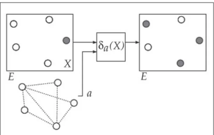
If a structuring function is a graph, we have b(x)={y∈E:d(y,x)≤1} (x∈E)

where E is the set of vertices of a graph and d(y,x) is the distance between y and x of this graph. See in Figure 7 an example of expansion based on neighborhood graphs2_.

2 _{The Figure 7 is simplified, the structuring function is given}

by neighbors of each corner of the graph.

Figure 7: Dilation by a flat structuring function, with r=1. 2.5 Images partition and labeled

We define partition image as the division of an image in partitions, where the union of all the partitions is the image and the intersection of two separate partitions is empty. The partitions are differentiated by different gray scale. See an example of partition image in Figure 8-a.

We also use a definition of approximately partition image, where there is a line at the intersection of any two adjacent partitions. See an example in Figure 8-b.

Figure 8: (a) Partition image and (b) partition image, with dividing line.

From the partition image it is possible to create a neighborhood graph, where vertices can be the centroid of each partition and the edges connect the two neighboring partitions. In this paper, we will build neighborhood gra-phs from an image partition using morpho-logical operators, as detailed in the section 3.

3 CONSTRUCTION OF NEIGHBORHOOD GRAPHS BY MORPHOLOGICAL

OPERATORS

We present the construction of a neighbor-hood graph as follows: consider with input ima-ge of the segmentation of human muscle cells, Figure 9-(a). The Figure 9-(b) shows the dilation of the centroid of each cell, for better viewing. So, a centroid of a cell is represented by a pixel and the set of all centroids will define the set of edges of the graph.

Figure 9: (a) input image and (b) centroid of each cell. To identify each edge of the neighborhood graph, consider the images labeled and water-shed, Figure 10 (a) and (b), respectively. This view of the numbers of the labels was inspired in the software documentation mmoph, in de-monstration mmdblob - Demonstrate blob mea-surements and display3_.

3 _{www.mmorph.com}

Figure 10: (a) label image and (b) watershed image.

Figure 11 defines the image f labeled of the negated watershed. This image, disregarding the numbers of labels, will be used to find the neighbors of each label.

Figure 11: Label negated the watershed, with the numbers representing the gray levels of each label.

The Figure 12 presents a binary image, f₁, only with the first label's image f. In Figure, g₁ is the dilation of f₁ by a structuring function b=3 3, then, it does the intersection with f subtracted of f₁, i.e.,

g₁=(f₁∧δ_b(f₁))–f₁.

The image c₁ is the reconstruction of g₁ res-tricted to f, i.e.,

c₁=(f⊕_g

1

b)∞.

This image c₁ defines the neighbors edges of the first label's image f.

Figure 12: f1 binary image the first label's image f, g1=(f1∧δb(f1))

Figure 13 repeats this transformation to the label 8. So, the construction of the neighbor-hood graph of the image f can be generalized as follows: let N be the number of vertices (or labels of f) of the graph. Then ∀i∈N and N≥2, let Ni be all the edges to neighboring vertex i,

defined as follows:

Ni = ci,

where ci returns to the gray scale of image ci.

Figure 13: fi binary image the first label's image f, gi=(fi∧δb(fi))

–f_i, reconstruction c_i=(f⊕g_ib)∞_.

We present the following neighborhood graph generated from the image of Figure 9, where the first line defines a structuring function. The second line defines size image, (x,y) and the type graph. The third line defi-nes the number of nodes of the graph, in this case with 18 vertices. The following 18 rows define each edge (number of neighbors, value of the vertex, coordinates (x,y) and its neighbors).

Figure 14 illustrates the file before drawing a graph, along with the image of the targeted cell of human muscle.

Figure 14: Illustration of graph linking the cells.

MM_STRUCT % defines a structuring function

2 128 128 1 % defines size image 128x128 and the type graph 18 % number of nodes of the graph

% number of neighbors; value of the vertices; x ; y ; its neighbors 2 0 28 5 2 4 %%%% Figure 12 4 0 56 5 1 3 4 7 4 0 80 17 2 5 7 9 5 0 22 25 1 2 6 7 8 3 0 108 34 3 9 10 3 0 6 44 4 8 13 6 0 55 46 2 3 4 8 9 11 5 0 27 57 4 6 7 11 13 %%%% Figure 13 6 0 78 59 3 5 7 10 11 12 4 0 113 64 5 9 12 14 7 0 52 83 7 8 9 12 13 15 16 5 0 91 86 9 10 11 14 15 5 0 21 90 6 8 11 16 17 4 0 114 103 10 12 15 18 5 0 73 112 11 12 14 16 18 4 0 44 122 11 13 15 17 2 0 10 124 13 16 2 0 104 124 14 15 4 CONCLUSION

In this paper we have presented a way to build neighborhood graphs by morphological operators. This method used a segmented ima-ge as input, containing objects that define the graph vertices. The edges of the graph were defined by the neighborhood between these objects, defined by the watershed.

Using the basic operations in images of in-tersection, subtraction and negation, in addi-tion to the operators morphological of dilaaddi-tion, reconstruction and labeling, it was possible to build a graph from the watershed, represen-ting the edges of each vertex.

REFERENCES

[1] G. J. F. BANON and J. BARRERA.

Decomposi-tion of mappings between complete lattices by mathematical morphology, Part I: general lattices. Signal Processing, 30,:299-327, 1993,. [2] J. BARRERA, F. A. ZAMPIROLLI, and R.A. LOTUFO.

Morphological operators characterized by neighborhood graphs. In L. H. de FIGUEIREDO

and M. L. NETTO, editors, SIBGRAPI’97 - X

Brazilian Symposium on Computer Graphic and Image Processing, pages 179-186. IEEE Com-puter Society, October 1997.

[3] J. BONDY and U. MURTY. Graph theory with

applications. The Macmillan Press LTD, London, 1976.

[4] B. CHAZELLE and H. EDELSBRUNNER. An

improved algorithm for constructing kth _{- order}

Voronoi diagrams. ACM, 16:228-234, 1985. [5] T. CORMEN, C. LEISERSON, and R. RIVEST.

Introduction to Algorithms. The MIT Press, Cambridge, Mass., 1990.

[6] J. CRESPO. Morphological connected filters

and intra-region smoothing for image segmentation. Novembre 1993.

[7] L. FIGUEIREDO and P. CARVALHO. Introdução à

Geometria Computacional. Instituto de Matemá-tica Pura e Aplicada, Rio de Janeiro-RJ, 1991. [8] L. GUIBAS and J. STOLFI. Primitives for the

manipulation of general subdivisions and the computation of Voronoi diagrams. ACM Transactions on Graphics, 4 - N.2, April:74-123, 1985.

[9] R. JONES. A graph-based segmentation of

eucalypt pulpwood images. CSIRO Division of Mathematics and Statistics North Ryde -Australia, 1996.

[10] M. JÜNGER, G. REINEL, and D. ZEPF.

puting correct Delaunay triangulations. Com-puting, 47:43-49, 1991.

[11] D.-T. LEE. On k-nearest neighbor Voronoi

diagrams in the plane. IEEE - Transactions on Computers, C-31:478-487, 1982.

[12] F. P. PREPARATA and M. I. SHAMOS.

Compu-tational Geometry: an Introduction. Springer Verlag, 1985.

[13] P. REZENDE and J. STOLFI. Fundamentos de

Geometria Computacional. IX Escola de Compu-tação, Recife-PE, 1994.

[14] P. SALEMBIER and J. SERRA. Flat Zones

Filetring, Connected Operators, and Filters by Reconstruction. IEEE Transactions on Image Processing, 4(8):1153-1160, August 1995.

[15] J. SERRA. Image Analysis and Mathematical

Morphology. Academic Press, London, 1982. [16] J. SERRA, editor. Image Analysis and

Mathematical Morphology - Volume II : Theoretical Advances. Academic Press, London, 1988.

[17] F. Y. SHIH and O. R. MITCHELL. A

mathe-matical morphology approach to Euclidean distance transformation. IEEE Transactions on Image Processing, 1:197-204, 1992.

[18] L. VINCENT. Graphs and mathematical

morphology. Signal Processing, 16:365-388, April 1989.

[19] F.A. ZAMPIROLLI. Operadores morfológicos

baseados em grafos de vizinhanças - uma ex-tensão da mmach toolbox. Master's thesis, Departamento de Ciência da Computação, Ins-tituto de Matemática e Estatística, Unversidade de São Paulo, CP 66.281, CEP 05315-970, São Paulo, SP, Brazil, April 1997.

These graphs can be used for the construc-tion of morphological operators based on neighborhood graphs [19]. This model permits a complete equality between theory and imple-mentation, and leads to a natural polymorphic extension of morphological image processing software. Using the conceptual model

pro-posed we have implemented an extension of the MMach toolbox and used it for the solution of some image analysis problems: detection of fracture lines in porous materials, iden-tification of non productive regions of Euca-lypt pulpwood and segmentation of the faces of a block.