Explainable artificial intelligence

(1)

UNIVERSIDADE DE LISBOA FACULDADE DE CI ˆENCIAS DEPARTAMENTO DE INFORM ´ATICA

-LEARNING DECISION SETS WITH SAT

Filipe In´acio da Costa Pereira

MESTRADO EM ENGENHARIA INFORM ´

ATICA

Especialização em Interação e Conhecimento

Dissertac¸˜ao orientada por:

Prof. Doutor Jo˜ao Paulo Marques da Silva

(2)

(3)

Acknowledgments

My first acknowledgement will go to my advisor Jo˜ao Marques Silva, not only for being an expert in the fields of Logic but also because he never hesitated to help or lend an ear. Without him, I wouldn’t have as much of a good time as I had doing this. Thanks to him, I was also able to attend the Federated Logic Conference 2018, in Oxford. As he always said, ”Plans are worthless, but planning is everything”. Also invaluable was Alexey Ignatiev, his early tips gave me the head start necessary to dive in the world of logic and research. I would also like to thank United Technologies Research Center for my research grant.

To my family, my mother, Maria Isabel, who sacrificed herself so I could be who I want, to my father, Joaquim Pereira, who paid my university fees, to my brother, Ti-ago Pereira, who was always there and finally, my two beautiful nephews, Miguel and Leonardo.

To the people that helped me with the timeline of my thesis. Specifically, in delaying it. Procrastination did wonders. To the people that have been present since my high school, my group ”Spiders”, Sebastião Peixoto, Rafael Pacheco, Bernardo Pina, Henrique Vale, Tiago Ferreira, Pedro Bengaló, Pedro Pereira and João Pereira.

To the faculty group, ”Questões da Vida”, João Antunes, João Cardoso, João Batista, João Rodrigues and Dharmite Prabhudas.

Finally, to the grammar police, Margarida Penedos, who LOVED my use of commas and once again, Jo˜ao Batista.

I think that’s enough sissy stuff. ”Bla bla bla”and to everyone, once again, thank you.

(4)

(5)

(6)

(7)

Resumo

A Inteligência Artificial é um tema de investigação fulcral no crescimento tecnológico e com um forte impacto desde a sua criação na conferência de Darmouth, em 1956, onde foi proposta a seguinte asserção sobre a inteligência artificial: “Todos os aspetos da apren-dizagem ou qualquer outra carater´ıstica de inteligência pode ser tão precisamente descrita que uma máquina pode ser feita para a simular”. Com o constante aumento de informação (Big Data) ao longo dos anos, temos modelos cada vez mais eficientes que em poucos se-gundos nos informam da sua predição sobre um dado conjunto de input, dos quais se destacam os Black Box Models, sendo estas as técnicas com melhores resultados e com maior complexidade. Infelizmente, estes não nos conseguem fornecer uma explicação para a sua predição, o que pode ser uma enorme desvantagem para nós seres humanos. Explainable Artificial Intelligence, que visa associar explicações a decisões feitas por agentes autónomos, quebra esta falta de transparência. Visto que para a tomada de de-cisões é necessário mais que uma etiqueta, será bastante útil uma explicação, criando assim uma relação de confiança com o modelo implementado.

Irão ser apresentados conceitos preliminares tais como o problema de satisfação, o problema da classificação, complexidade, problemas MaxSAT, subconjuntos de satisfia-bilidade máximos e subconjuntos de correção m´ınimos. Um dos objetivos é apresentar uma base de conhecimento sobre Explainable Artificial Intelligence, que relaciona uma forte componente de vários modelos e frameworks e se encontra dividida em duas grandes componentes: a de criação de modelos que já são interpretáveis por si ou a de criação de frameworksque justificam e interpretam predições escolhidas de quaisquer modelos. Os modelos interpretáveis podem ter uma abordagem heur´ıstica ou exata (com lógica). Den-tro destes modelos, são explorados mais a fundo os Conjuntos de Decisão, sendo estes os mesmos em que o nosso trabalho se baseia e comparada a sua eficácia com a nossa abordagem

As frameworks baseadas na interpretação e justificação de predições são também muito importantes pois permitem a justificação de qualquer predição de um modelo, de forma fiável e entend´ıvel por seres humanos. A maioria deste trabalho é focado em redes neuronais, sendo estes os modelos com melhor precisão mas sem justificação associada a cada predição. Também é estudado o problema de minimização de árvores de decisões. Este paper refere um modelo que, usando uma árvore fixa dada, consegue minimizar o

(8)

número de nós. Um dos problemas a notar é uma grande complexidade de espaço que não permitiu resultados fiáveis ou a existência dos mesmos. Os papers “Interpretable De-cision Sets” e “Minimizing DeDe-cision Tree Size as Combinatorial Optimization” foram a base da abordagem de lógica no mundo de Aprendizagem Automática.

Nesta tese será feita a descrição e análise da implementação de dois modelos inter-pretáveis (Conjunto de Decisão e Árvores de Decisão) baseados em lógica, através de Solucionadores SAT (Satisfiability) ou SMT (Satisfiability Modulo Theories). Este traba-lho foi motivado por uma análise em detalhe de trabatraba-lho na área de Inteligência Artificial Interpretável, com o propósito de procurar aplicações de lógica neste dom´ınio.

Os Conjuntos de Decisão têm tido um progresso formidável nestes últimos anos e con-seguem providenciar explicações sucintas e precisas. Estes são conjuntos de declarações “If-then”. Uma regra é constitu´ıda por um tuplo (π, c), em que π é um conjunto de itens e c a classe atribu´ıda, e é interpretada da seguinte maneira: SE os literais em π forem verda-deiros, ENT ÃO escolha a classe c. Um exemplo duma regra é: “Vacation:1 → Hike: 1”. Existem listas/conjuntos de decisão (que impõe ordem e estão conectados por declarações “else”) e listas/conjuntos de decisão (que não necessitam de ordem). Apesar de à partida os últimos aparentarem ser mais interpretáveis, com eles estão relacionados problemas tais como a sobreposição de regras.

A ferramenta desenvolvida é denominada de MINDS e a nossa abordagem de Con-juntos de Decisão começa com uma definição de conceitos importantes, baseados em trabalho anterior [1]. Conceitos como itemsets, regras, regras de definição e sobreposição de regras (quer seja no dataset ou no espaço de atributos) são explicados. A geração de explicações sucintas também é esclarecida. A nossa abordagem requer que os datasets estejam devidamente binarizados e considerando que maioria dos datasets não se encon-tra assim, serão aplicadas técnicas de ”one-hot encoding”. A binarização de um dataset implica transformar atributos categóricos em vetores binários mas esta aumenta ligeira-mente a complexidade de espaço do nosso modelo devido ao aumento de atributos. Os vários problemas de otimização do MINDS são abordados e apresentados a explicação da sua complexidade, tais como as variáveis e restrições de cada modelo. Cada mo-delo terá também um exemplo de um Conjunto de Decisões. A aprendizagem de Con-juntos de Decisão foca-se no dataset e o objetivo é passar através do mesmo, criando variáveis e restrições e atribuindo valores às mesmas com um solucionador SAT/SMT, permitindo a minimização do número de regras (ou Formas Normais Disjuntivas) para cada representação de classe binária (c0 e c1) e evitando sobreposição nas regras, sendo

estas pelo dataset ou pelo espaço de atributos, mantendo assim explicações interpretáveis e com precisão perfeita. Trabalho anterior [1] focou-se apenas em sobreposição de re-gras no dataset, na nossa abordagem existe o foco em retirar a sobreposição de rere-gras no espaço de atributos. Também é realizada uma abordagem de quebra de simetrias (pois existe uma falta de ordem nas regras), de forma a melhorar o espaço das restrições e obter

(9)

mais desempenho. Impor uma ordem implica uma redução na complexidade e não afeta a precisão.

Para Árvores de Decisão existem abordagens práticas realizadas com procura heur´ıstica para a aprendizagem das mesmas. A nossa abordagem de Árvores de Decisão com SAT, cria restrições que codificam uma árvore binária válida e, por sua vez, restrições que ga-rantam que a árvore de decisão seja perfeita (100% precisa) enquanto classifica os exem-plos no dataset. Se as restrições forem válidas quando passadas por um solucionador SAT, este irá retornar uma árvore de decisão válida e otimizada. Tal como na abordagem anterior, também é usada uma maneira de quebrar simetrias aqui: ao assegurar que aos ramos da esquerda sejam concedidos um atributo com o valor 0 e aos ramos da direita com o valor 1. Este modelo desenvolvido tem uma complexidade muito inferior ao do paper ”Minimizing Decision Tree Size as Combinatorial Optimization”e não requer uma árvore de decisão fixa.

Houve também investigação extensiva na comparação dos modelos referidos, tais como o IDS, JRIP, PRISM, CN2 e modelos do MINDS. Uma grande parte dos data-sets usados nos resultados experimentais eram inconsistentes, tendo várias ocorrências do mesmo exemplo com classes atribu´ıdas diferentes. A forma de resolver tal situação foi atribuir a classe C ao subconjunto maior. Os nossos modelos necessitam de datasets consistentes, senão as restrições nunca seriam solucionadas (pois seria imposs´ıvel chegar a 100% de precisão). Os testes foram realizados em 49 datasets e impostos um tempo limite de 600 segundos. Estes datasets tinham uma grande quantidade de linhas, atributos e valores distinctos em cada atributo. Os modelos SAT têm como objetivo minimizar o número de regras mas de forma a tornar os conjuntos de decisões mais concisos, foi re-alizada uma técnica de enumeração de subconjuntos de correção m´ınimos. A avaliação foi feita nos 49 datasets, baseando os critérios no número de regras e literais, precisão e tempo. Existe uma pequena discussão das novas Regulações Europeias de Proteção de Dados, pois estas legislações criam o direito de ter uma explicação e restringem perfi-lagem. Concluindo, existe uma visão geral positiva devido aos resultados experimentais obtidos, possivelmente com um objetivo futuro de tornar os modelos mais eficientes e com menos literais de forma a competir com outros modelos.

Palavras-chave: Inteligência Artificial Explicável, Modelos Interpretáveis,

Interpretação e Justificação de Predição, Conjunto de Decisão, Solucionadores SAT.

(10)

(11)

Abstract

Artificial Intelligence is a core research topic with key significance in technological growth. With the increase of data, we have more efficient models that in a few sec-onds will inform us of their prediction on a given input set. The more complex techniques nowadays with better results are Black Box Models. Unfortunately, these can’t provide an explanation behind their prediction, which is a major drawback for us humans. Explain-able Artificial Intelligence, whose objective is to associate explanations with decisions made by autonomous agents, breaks this lack of transparency. This can be done by two approaches, either by creating models that are interpretable by themselves or by creating frameworks that justify and interpret any prediction made by any given model.

This thesis describes the implementation of two interpretable models (Decision Sets and Decision Trees) based on Logic Reasoners, either SAT (Satisfiability) or SMT (Sat-isfiability Modulo Theories) solvers. This work was motivated by an in-depth analysis of past work in the area of Explainable Artificial Intelligence, with the purpose of seeking applications of logic in this domain.

The Decision Sets approach focuses on the training data, as does any other model, and encoding the variables and constraints as a CNF (Conjuctive Normal Form) formula which can then be solved by a SAT/SMT oracle. This approach focuses on minimizing the number of rules (or Disjunctive Normal Forms) for each binary class representation and avoiding overlap, whether it is training sample or feature-space overlap, while maintaining interpretable explanations and perfect accuracy.

The Decision Tree model studied in this work consists in computing a minimum size decision tree, which would represent a 100% accurate classifier given a set of training samples. The model is based on encoding the problem as a CNF formula, which can be tackled with the efficient use of a SAT oracle.

Keywords: Explainable Artificial Intelligence, Interpretable Models, Prediction Interpretation and Justification, Decision Sets, SAT Solvers.

(12)

(13)

List of Figures

2.1 Decision Tree for Hike Dataset . . . 7

3.1 IDS vs BRL on a medical diagnosis dataset . . . 11

3.2 Falling Rule List for mammographic mass dataset . . . 11

3.3 MP92 Circuit Representation . . . 13

3.4 Neural Network with innate explanations . . . 13

3.5 Control Procedure for Unordered List Learner . . . 16

3.6 Explanation of predictions by LIME . . . 18

3.7 BETA two-level decision set on depression dataset . . . 18

3.8 Two explanations of Deep Learning predictions . . . 19

3.9 Bessiere Benchmarks . . . 22

5.1 Experimental Results - Rule vs Literals . . . 45

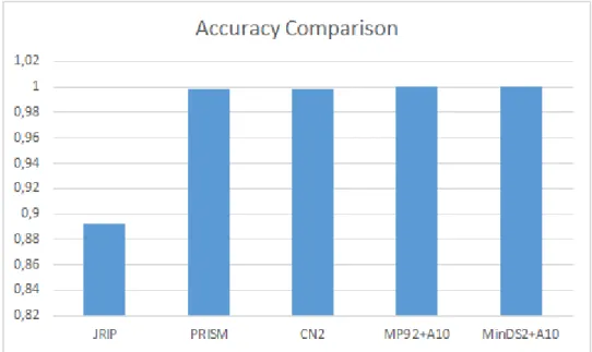
5.2 Experimental Results - Accuracy . . . 46

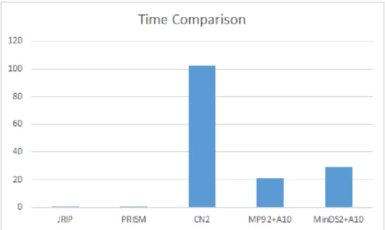
5.3 Experimental Results - Time . . . 47

(18)

(19)

List of Tables

2.1 A Classification Example . . . 6

3.1 Formulation of the problem of finding the Smallest Decision Tree . . . . 20

3.2 Space complexity of the SAT-Based Encoding of Smallest Decision Tree problem . . . 21

4.1 HaveBeer Dataset . . . 28

4.2 Description of propositional variables . . . 35

5.1 Number of solved instances per model (out of 49) . . . 41

5.2 Number of solved instances per model (out of 49) - Alternate setup . . . . 41

A.1 Weka - JRIP Benchmarks . . . 58

A.2 Weka - PRISM Benchmarks . . . 59

A.3 Orange - Unordered List Learner Benchmarks . . . 60

A.4 MinDS – MP92 Benchmarks . . . 61

A.5 MinDS – MP92 with A10 Benchmarks . . . 62

A.6 MINDS - SAT Benchmarks . . . 63

A.7 MinDS - SAT with A10 Benchmarks . . . 64

A.8 MinDS – MinDS1 Benchmarks . . . 65

A.9 MinDS - MinDS1 with A10 Benchmarks . . . 66

A.10 MinDS - SMT (Z3 Solver) Benchmarks . . . 67

A.11 MinDS - SMT (Yices2 Solver) Benchmarks . . . 68

(20)

(21)

Chapter 1 Introduction

Artificial Intelligence has been the subject of research for decades and its impact has been far-reaching since its birth on the Dartmouth Conference, in 1956. The proposal for the conference included this assertion: “every aspect of learning or any other feature of intelligence can be so precisely described that a machine can be made to simulate it” [2]. From a simple game AI to self-driving cars, artificial intelligence is of great importance to technological advancement.

Machine Learning, a field of Artificial Intelligence, gives computers the ability to learn from data. Although very useful, most machine learning models nowadays are black boxes whose sole purpose is to predict, but we, as curious humans, need more than a (class) label. We need explicit knowledge in order to trust our models. With this in mind, comes Explainable Artificial Intelligence in which we understand why (and why not) some prediction was chosen, when the model will succeed (and when it will fail) and know when to trust the model itself (and why it erred) [3].

1.1 Motivation

Explainable Artificial Intelligence (XAI) is a promising and upcoming field of research [1, 4–6] with far-reaching expected impact. It also has an ongoing research program [3] and furthermore, the new European General Data Protection Regulations are enforcing au-tomated generation of explanations [7]. There is also a number of meetings on computing machine learning models [8–10]. In a general sense, XAI aims to associate explanations with decisions made by autonomous agents. Even though there is an adequate amount of research on Artificial Intelligence [11, 12] there needs to be a shift in favor of Explainable Artificial Intelligence. A larger appeal needs to be made for the creation of XAI since the lack of transparency is a major drawback [13].

(22)

Chapter 1. Introduction 2

1.2 Objectives

The main purpose of this thesis is to summarize ongoing efforts in XAI by creating a knowledge base, assess models referenced and other available tools and, finally, create an Interpretable Model using logic-based methods with good performance, accuracy and a solid way of explaining decisions. This shall be achieved by:

• Developing a Knowledge Base of XAI through reference mapping;

• Understanding XAI models, assessing them and summarizing their pros and cons; • Creating an Interpretable Model, with performance and accuracy comparable to

existing classifiers, using logic-based reasoners;

• Comparing the proposed models against the state of the art tools in rule based learn-ing, such as IDS, Orange, and Weka.

1.3 Contributions

With the completion of this thesis, we have achieved two main contributions:

• Bringing a more detailed logic approach to the world of Decision Sets, explain-ing different optimization problems with rigorous variables and constraints, with our models maintaining perfect accuracy when tested on the same training dataset, while minimizing the number of rules and providing approaches to minimize the number of literals as well, in order to bring an overall interpretable decision set; • Learning an ideally minimum size Decision Tree with SAT techniques, with precise

variables and constraints, helping us guess valid binary trees and verify whether or not they classify all the examples correctly.

1.4 Publications

During the period of my Master Thesis, I co-authored the following papers, which were accepted for publication in CORE A* conferences:

• A SAT-Based Approach to Learn Explainable Decision Sets, authored by A. Ig-natiev, F. Pereira, N. Narodytska and J. Marques-Silva, which has been accepted for publication at IJCAR 2018 [14].

• Learning Optimal Decision Trees with SAT, authored by N. Narodytska, A. Ignatiev, F. Pereira, and J. Marques-Silva, which has been accepted for publication at IJCAI 2018 [15].

(23)

Chapter 1. Introduction 3

1.5 Document Organization

The document is organized as follows:

• Chapter 2 - Preliminaries: This chapter will revolve around the core concepts of this Thesis, like Boolean satisfiability, the Classification Problem, Complexity and the MaxSAT problem, minimal correction subsets and maximal satisfiable subsets. • Chapter 3 - Related work: This chapter will focus on Interpretable Models and

Frameworks based on Prediction Interpretation and Justification. There is also a section explaining the Smallest Decision Tree Problem [16], which is the inspiration for the logic-based model.

• Chapter 4 - Learning Decision Sets & Decision Trees with SAT: This chapter will explain in detail the work done throughout the duration of this thesis, from the design to the analysis of algorithms, as well as my contribution to the work done. • Chapter 5 - Experimental Results: This chapter will show experimental results of

the algorithm implemented in comparison with other tools.

• Chapter 6 - Discussion: This chapter will present a simple summary of the thesis, some final conclusions, address how the new legislation might affect the area of machine learning and what’s to be expected of future work.

(24)

(25)

Chapter 2 Preliminaries

This section provides an overview of Boolean Satisfiability (SAT), the Classification Prob-lem, Complexity, the MaxSAT ProbProb-lem, Minimal Correction Subsets and Maximal Satis-fiable Subsets.

2.1 Boolean Satisfiablity

We assume notation and definitions standard in the area of SAT [17]. Formulas are rep-resented in Conjunctive Normal Form (CNF) and defined over a set of variables X = {x1, ..., xn}. A formula F is a conjunction of clauses, a clause is a disjunction of literals

and a literal is a variable xi or its respective complement ¬xi. The Satisfiability Problem

is the task of determining if a truth assignment (assignments of 0 or 1 to each variable) exists that makes a given propositional formula true.

2.2 Classification Problem

First of all, [R] is used to denote the set of natural numbers {1, ..., R} and for a point f in some K-dimensional space, the rth _{coordinates is given by f [r]. Following the notation}

used in earlier work [16], we consider a set of features F = {f1, ..., fk} which are

con-sidered to be binary, taking the value of either 0 or 1. When needed, the standard one hot encoding is used to handle non-binary categorical features, which turns labels into inte-gers and inteinte-gers into binary vectors. Since all features are binary, a literal on a feature fr

will be represented as frwhen the feature takes value 1 or ¬frwhen it takes value 0. The

feature space is represented by U _,QK

r=1{fr, ¬fr}.

In order for a classifier to learn, it must begin from given training data E = {e1, ..., em}.

Examples are associated with classes taken from a set of classes C but since these models focus mostly on binary classification (C = {co, c1}), we will associate co with 0 and c1

with 1. E is split into E+and E−, denoting examples classified as positive and negative, respectively. Each example eq ∈ E is represented as a 2-tuple (πq, cq), in which πqdenotes

(26)

Chapter 2. Preliminaries 6

the literals associated with the example and cq ∈ {0, 1} is the class to which the example

belongs to. A literal lron a feature fr, lr ∈ {fr, ¬fr}, discriminates an example eqif and

only if πq = ¬lr, i.e the feature takes the value opposite to the value in the set of literals

of the example.

Given the dataset presented at Table 2.1, two possible example decision sets are pre-sented below, one with overlap1 _{and another one without (the notion of overlap will be}

further discussed in 4.1.1), followed by an example decision tree and a brief explanation on how to present sample e1:

Ex Vacation(V) Concert(C) Meeting(M) Expo(E) Hike(H)

e1 0 0 1 0 0 e2 1 0 0 0 1 e3 0 0 1 1 0 e4 1 0 0 1 1 e5 0 1 1 0 0 e6 0 1 1 1 0 e7 1 1 0 1 1

Table 2.1: A Classification Example

A decision set with some overlap would be:

If¬ MeetingthenHike

If¬ Vacationthen¬ Hike A decision set with no overlap would be:

IfVacationthenHike

If¬ Vacationthen¬ Hike

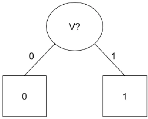
A decision tree for the dataset would be:

1_{Overlap between two rules assesses whether the set of points covered by two rules intersect (an example} being the set of points (¬V, ¬C, ¬M, ¬E) for the decision set with overlap).

(27)

Figure 2.1: Decision Tree for Hike Dataset

The set of binary features is {f1, f2, f3, f4}, in which f1is the feature Vacation (V), f2

the feature Concert (C), f3 the feature Meeting (M) and f4 the feature Expo (E). To this

end, the example e1is represented by the tuple (π1, c1) with π1 = {¬f1, ¬f2, f3, ¬f4} and

c1 = 0. Moreover, literals {f1, f2, ¬f3, f4} discriminate e1. Note that U = {V, ¬V } ×

{C, ¬C} × {M, ¬M } × {E, ¬E}.

The objective of this classification is to learn a function which matches the training data and generalizes suitably well on unseen test data. In this thesis, we seek representa-tions of this function corresponding Decision Sets (DS) and Decision Trees (DT).

2.3 Complexity

Throughout this thesis, standard computational complexity definitions will be assumed. These include the well-known classes of NP-complete and NP-Hard problems. Additional classes of complexity, including different levels of the polynomial hierarchy, will also be assumed. The interested reader should check [18] for additional detail and information.

2.4 MaxSAT problem, Minimal Correction Subsets and

Maximal Satisfiable Subsets

MaxSAT is an optimization version of SAT [19], and a MaxSAT problem consists of find-ing an assignment that satisfies the maximum number of clauses of a given unsatisfiable formula. The MaxSAT problem is well known to be NP-hard since SAT is polynomial time reducible to MaxSAT. A generalization called Partial MaxSAT exists, such that a subset of clauses that must be satisfied are named hard clauses, as for the remaining ones that may or may not be satisfied are named soft clauses. In a variant of the MaxSAT prob-lem, named Weighted MaxSAT, each soft clause has an associated weight and the goal

(28)

becomes to maximize the sum of the weights of the satisfied soft clauses while satisfying all the hard clauses.

Based on earlier work [20], the largest Maximal Satisfiable Subset (MSS) represents a solution to the MaxSAT problem, which can also be represented by its complemented called the smallest Minimal Correction Subset (MCS).

Given a set of clauses Z, which can be presented by z or zi, with i = {1, ..., m},

where m = |Z|, we have the following definitions:

• A MCS is defined as follows: C ⊆ Z, iff Z \C is satisfiable and ∀z ∈ C, Z \(C \{z}) is unsatisfiable.

• A MSS is defined as follows: S ⊆ Z, iff S is satisfiable and ∀z ∈ Z \ S, Z ∪ {z} is unsatisfiable.

In order to illustrate these concepts, we present the following example. The hard and soft clauses are, respectively: H = {(¬x1∨¬x2), (¬x1∨¬x3), (¬x4∨¬x5), (¬x4∨¬x6)},

S = {(x1), (x2), (x3), (x4), (x5), (x6)}.

Given the previous formula Z, MaxSAT ≡ 4 with the MSS being the set of clauses {(x2), (x3), (x5), (x6)} and MCS being the set of clauses {(x1), (x4)} such that the union

of both equals Z. We pick this solution because it satisfies all the hard clauses and the largest number of soft clauses. Therefore, this solution has the lowest number of soft clauses left unsatisfied.

(29)

Chapter 3 Related Work

This chapter provides a first take at an annotated bibliography of papers that were deemed relevant to the thesis’ main area of work.

In order to better represent the related work in XAI, a decision was made to categorize earlier work into two main areas, based on [21], those being Interpretable Models and Prediction Interpretation and Justification. Furthermore, the addition of a subsection was made in order to summarize the Smallest Decision Tree problem [16] that inspired a logic approach to machine learning.

The denotation Decision Lists and Rule Lists mean the same with these being ordered sets of ”if-then” rules, furthermore, the denotation Decision Sets and Rule Sets also mean the same with these being unordered sets of ”if-then” statements. More information is available in section 4.1.

3.1 Interpretable Models

There are a wide variety of interpretable models, whose performance and accuracy is high, but nowhere near as high as black box models. The trade-off is being able to provide explanations behind their predictions without the help of an additional framework. There is also a subsection to present other available tools, that are going to be assessed later in 5.5. Some examples are:

The work of Letham et al. [4] This paper aims to produce models that are highly accu-rate and interpretable by humans. These models are Bayesian Rule Lists, which consist of series of ordered if-then statements that discretize a high-dimensional, multivariate fea-ture space into a series of simple, readily interpretable decision lists. Based on statistical rule learning, BRL produces a posterior distribution over permutations of if-then rules, starting from a large, pre-mined set of possible rules. A major source of BRL’s practical feasibility is the fact that it uses these pre-mined rules, which reduce the model space to that of permutations of rules as opposed to all possible sets of splits thus reducing

(30)

Chapter 3. Related Work 10

the space complexity drastically. The following rule list (taken from [4] is based on the Titanic Dataset:

If male and adult then survival probability 21% (19%-23%) else if 3rd class then survival probability 44% (38%-51%) else if 1st class then survival probability 96% (92%-99%) else survival probability 88% (82%-94%)

This model uses a statistical rule learning approach while ours uses an exact approach. Although BRL’s performance is highly based on subsampling datasets, it doesn’t reach a high accuracy on most of them, despite that, it is an innovative way to build decision sets.

The work of Lakkaraju et al. [1] This paper presents a framework for building pre-dictive models that aim to be highly accurate and interpretable, but on our benchmarks (5.3) it failed to do so. The model created is a Decision Set which is simple, concise, interpretable and represents an unordered set of if-then rules. If a given feature is not found on the rules, then a default rule is used. Finding a model within a space designed for interpretability takes some time, so in order to work on big data, a pre-mined space of rules is needed.

A decision set (S) is a set of rules of the form (π, c), where π is an itemset and c is a class label. An itemset π is a filter of data points, defined as a conjunction of one or more predicates of the form (attribute, operator, value) i.e (x1 > 5). The attribution of a class

label c is as follows: If attribute values x satisfy exactly one itemset πi, then the class

label is the corresponding ci. If x satisfies zero itemsets, then it is attributed to a default

label. Finally, if x satisfies more than one itemset, it is assigned a class label c based on a tie-breaking function.

IDS tries to optimize interpretability and accuracy. For interpretability, IDS tries to: • Lower the number of rules for easier reading, which is checked by size(S);

• Have a decent number of predicates in a rule, which can be checked by Length(r) for some rule r = (π, c);

• Have a way to verify the set of data points which are satisfied in the Decision Set S, defined on a per-rule basis by using Cover(r) for a rule r = (π, c), which is the set of data points in S with attribute values x that satisfy the itemset π;

• Lower the overlap, measured by overlap(r, r0), for rules r = (π, c) and r0 = (π0, c0), which checks the set of data points that satisfy both π and π0. The measure is defined as: overlap(r, r0) = cover(r) ∩ cover(r0).

In order to optimize accuracy, a decision set must effectively predict class labels. So IDS tries to measure per-rule accuracy with:

• correct − cover(r), defined by: correct − cover(r) = {(x, y) ∈ cover(r)|y = c} which is the set of data points in S that satisfy π and belong to class c;

(31)

• incorrect − cover(r), defined by incorrect − cover(r) = cover(r) \ correct − cover(r), which is the set of data points in S that satisfy π but do not belong to class c.

Optimization of said decision sets usually involves Smooth Local Search [22].

Figure 3.1: Interpretable Decision Set (on the left) and a Bayesian Decision List (on the right) on the same medical diagnosis dataset (taken from [1])

The framework IDS 1 _{was provided and even with a simple dataset such as Titanic}

with the .TAB extension (provided in the src), it took a very long time to build a decision set, averaging around 240 seconds. As soon as we put it to test with our datasets, this framework failed to provide solutions, which are explained in 5.3. Although this was unforeseen, IDS provided us with the definitions important to our work.

The work of Wang et al. [23] This paper presents the model Falling Rule Lists which consist of an ordered list of if-then rules where the order of the rules determines which example should be classified first by each rule and the estimated probability of success (or risk) decreases monotonically down the list. In certain situations, actions need to be taken and prioritized based on risk. The decision process is natural for a human decision-maker but not for machine learning models. Thus, falling rule list contains the most at-risk ob-servation classified first. The model itself is quick to produce and serves a dual purpose: Ranking to form a predictive model and stratifying patients into decreasing risk sets. The model also aims to bring accuracy, interpretability, and computation. FRL builds the same way as Bayesian Rule Lists [4], with pre-mined itemsets.

Figure 3.2: Falling Rule List for mammographic mass dataset(taken from [23]) 1_{https://github.com/lvhimabindu/interpretable_decision_sets/}

(32)

The difference between Bayesian Rules Lists and Falling Rules Lists falls mostly on monotonicity and stratifying the most important cases first, the ones with a higher proba-bility of risk (seen in 3.2).

The work of Angelino et al. [5] This paper implements a custom discrete optimization technique algorithm for building rule lists over a categorical feature space. The branch-and-bound algorithm named CORELS consists of a systematic enumeration of candidate solutions by means of feature space searching and provides a highly accurate rule list. Summarizing, this algorithm finds a transparent model that is optimal within a particular pre-determined class of models and produces a certificate of its optimality. The class of rule lists assembled are from pre-mined frequent itemsets and the objective is to search for a rule list that minimizes a regularized function. It also uses binarized datasets, just like in our approach.

CORELS (Certifiably Optimal Rules Lists) provides: • An Optimal Solution;

• A Certificate of optimality;

• A Collection of near-optimal solutions and the distance between each one and the optimal one.

The following rule list, taken from [5], predicts two-year recidivism for the ProPublic dataset:

if (age = 23 - 25) and (priors = 2 - 3) then predict yes else if (age = 18 - 20) then predict yes

else if (sex = male) and (age = 21 - 22) then predict yes else if (priors > 3) then predict yes

else predict no

The work of Kamath et al. [24] Inductive reasoning is a method of reasoning in which the premises are viewed as supplying strong evidence for the truth of the conclusion. This model creates a function F : {0, 1}n → {0, 1} that maps input into an output, with this output being either 0 or 1, belonging respectively to the Off-set or On-set. The given func-tion is represented as a sum of product terms (Disjunctive Normal Form). Explanafunc-tions come from a logical form that is the disjunction of conjunction clauses. If the function F maps to 1, we can see which features have weight on the result based on the given input.

(33)

Figure 3.3: Circuit Representation of Boolean expression: y = x1¬x2 + ¬x1x2 (taken

from [24])

Inspired by this earlier work, one of our models was created based on this approach, which is further studied in section 4.1.2.1.

The work of Li et al. [6] This paper implements a novel architecture for deep learning that explains its reasoning behind each prediction. Contains an autoencoder, which is a type of neural network used to learn efficient data codings in an unsupervised manner, and a prototype layer where each unit of that layer stores a weight vector that resembles an encoded training input.

The autoencoder has both an encoder (that allows comparisons within the latent space) and a decoder (that allows visualization of the learned prototypes). The decoder allows for a quick visualization of prototypes based on our dataset i.e if we train on the MNIST dataset, it will show the learned numbers.

Figure 3.4: Network Architecture for Neural Network explanation (taken from [6])

(34)

ev-Chapter 3. Related Work 14

ery prototype to be similar to at least one encoded input, a term that encourages every encoded input to be close to at least one prototype and a term that encourages faithful reconstruction by the autoencoder. Their definition of a prototype is something very close or identical to an observation in the training set and a set of prototypes is representative of the whole dataset.

The work of Lou et al. [25] Complex models for regression and classification have high accuracy but are unfortunately no longer interpretable by users. Generalized Additive Models (GAM) are complex functions turned into one-dimensional components so, in a way, these combine single-feature models called shape functions through a linear function that can be easily interpreted by users (by understanding the contribution of individual features). The model is fitted to the following form: g(y) = f1(x1) + ... + fn(xn), where

g is a link function, fna shape function and xna feature.

In order to create these models, we need to select a shape function for individual fea-tures (these being regression splines or ensembles of trees) and select a learning method for the model (learning square for regression splines and gradient boosting/backfitting for ensembles of trees).

The work of Clos et al. [26] Automatically classifying text documents is an active re-search challenge in document-oriented information systems. However, current approaches are biased towards building complex black box algorithms focused on producing high ac-curacy predictions at the cost of not being able to explain the rationale behind their deci-sions. This paper contributes with RELEXNET, an architecture that models lexicons as naive gated recurrent networks. Lexicon-based classifiers offer a white-box alternative to these approaches by using a trivially interpretable additive model at the cost of classifica-tion accuracy. This model is evaluated on stance detecclassifica-tion and sentiment classificaclassifica-tion. Lexicons fill the need for XAI by offering a trivially interpretable additive model, where the probability of an instance belonging to a class is modeled as a weighted sum of the probabilities of each term of that class belonging to that class. Examining the terms of an instance and its weights allows us to understand a prediction.

3.1.1 Available tools

This subsection was created in order to reference three models that are going to be present in the Experimental Results section of this thesis. These models are going to be analysed in order to better understand how they compare with our models. All these models use a heuristic approach to rule learning.

Cohen’s Model [27] JRIP is a class from the Weka collection that implements a propo-sitional rule learner named Repeated Incremental Pruning to Produce Error Reduction

(35)

(RIPPER), which was proposed by William W. Cohen as an optimized version of IREP [27]. RIPPER is based on association rules with reduced error pruning (REP) which is a common technique used in decision tree algorithms. This model can use nominal and continuous features. JRIP follows this procedure:

Initialize Ruleset, RS = {} and for each class, do:

1. Building Stage: Repeat step 1.a) and 1.b) until the description length (DL) of the ruleset and examples is greater than the smallest DL met so far, or there are no positive examples, or the error rate ≥ 50%

(a) Grow Phase: Grow one rule by greedily adding antecedents to it until the rule is perfect.

(b) Prune Phase: Incrementally prune each rule and allow the pruning of any final sequences of the antecedents.

2. Optimization Stage: After generating the initial ruleset {Ri}, generate and prune

two variants of each rule Ri from randomized data using procedure 1.a) and 1.b).

One variant is generated from an empty rule and the other is created by greedily adding antecedents to the original rule. The variant with the smallest DL is selected as the final representative of Riin the rule set.

3. Delete rules from the ruleset that would increase the DL of the whole ruleset and add resultant ruleset to RS.

End do.

For more information on how the algorithm works, it is recommended to follow the footnote2_.

Cendrowska’s Model [28] PRISM is a class from the Weka collection that imple-ments a PRISM rule set for classification, which induces modular rules. This model only works with nominal attributes, can’t deal with missing values and doesn’t do any prun-ing. PRISM, although based on ID3, uses a different strategy to induce rules, avoiding problems associated with decision trees.

PRISM follows this procedure:

If the training set contains instances of more than one classification, then for each classification, cn, do:

1. Calculate the probability of occurrence, p(cn|αx), of the classification cn for each

attribute-value pair αx;

2. Select the αx for which p(cn|αx) is a maximum and create a subset of the training

set compromising all instances which contain the selected αx;

(36)

3. Repeat steps 1 and 2 for this subset until it contains only instances of class cn;

4. Remove all instances covered by this rule from the training set; 5. Repeat steps 1-4 until all instances of class cnhave been removed.

End do.

The difference between PRISM and ID3 is that PRISM focuses on finding only rele-vant values of attributes, while ID3 tries to find the attribute which is most relerele-vant over-all. ID3 also splits the training set into homogenous subsets (based on the most relevant attribute) while PRISM identifies subsets of a specific class.

Clark et al. Model [29] The Unordered List Learner CN2 algorithm induces a set of unordered rules. It is built on the Orange library, available for Python. It can work with numerical features but the binarization of these helps tremendously with accuracy. CN2 Unordered List Learner has a process of learning rules for each class individually.

The CN2 algorithm consists of two main procedures, a search algorithm performing a beam search for a good rule and a control algorithm for repeatedly executing the search heuristic. During the search procedure, CN2 must evaluate the rules searched, finding out which one is the best. CN2 has three different heuristics for this: Entropy, Laplace Accuracy and Weighted Relative Accuracy. By default, Laplace’s rule of succession is used as a measure and is defined by: LaplaceAccuracy = (nc+ 1)/(ntot+ k) where nc

is the number of examples in the predicted class c covered by the rule, ntot is the total

number of examples covered by the rule and k is the number of classes in the domain. Now that the best rule is found, CN2 executes the search heuristic until we complete a rule. The control procedure for CN2’s Unordered List Learner is shown in Figure 3.5.

(37)

The main modification for the Unordered List Learner is for it to iterate the search for each class, removing only covered examples of that class when a rule has been found, unlike the Ordered List Learner which must maintain the negative examples because each rule must discriminate all negative examples. Also, for each class, the Laplace heuristic must be applied differently. With ordered rules, the predicted class c is taken simply as the one with most covered examples in it but with unordered rules, the predicted class is fixed to be the class selected by the revised control procedure.

3.2 Prediction Interpretation and Justification

Instead of making interpretable models, some authors tried a different approach that is based on building a framework to explain decisions of any classifier. Some good examples are:

The work of Ribeiro et al. [30] Machine Learning models remain mostly black boxes and nowadays understanding the reasons behind a prediction is needed in order to assess trust. LIME is a novel explanation technique that explains (presenting textual or visual ar-tifacts) faithfully the prediction of any classifier by learning an interpretable model locally around the prediction.

The authors of this paper state that: “If the users do not trust a model or prediction, they will not use it.”. The statement is true for decision making problems (examples being a medical diagnosis or terrorism detection) since we need to trust the prediction.

The desired characteristics for LIME are interpretability, local fidelity, model-agnostic, and a global perspective. In order to provide explanations, we need to assess which ex-planation might be the best. A model g contains a domain of {0, 1}d0 _{which is the}

ab-sence/presence of interpretable components (these can be words or a patch of contiguous pixels). In classification, we have a function f (x) which is the probability that x belongs to a certain class and πx(z) is a proximity measure between an instance z to x.

Explana-tions by LIME are produced by the following formula:

ξ(x) = argmin

g∈G

L(f, g, πx) + Ω(g)

The objective is to minimize L (which is a measure of how unfaithful g is in approx-imating f in the locality defined by πx) while maintaining Ω (which is the measure of

(38)

Figure 3.6: Explanation of Individual Predictions (taken from [30])

The work of Lakkaraju et al. [31] This paper proposes a model-agnostic framework, named Black Box Explanations through Transparent Approximations (BETA) that aims to explain any black box classifier while simultaneously optimizing fidelity of the model and the interpretability of the explanation.

The goal is to explain the behavior of any given black box classifier as a whole instead of just reasoning about its individual predictions. To this end, the framework constructs a small number of compact two-level decision sets, each of which captures the behavior of the given black box model in certain parts of the feature space. The framework also allows the user to define input, allowing him to explore the black box model.

The representation chosen is a two-level decision set (Figure 3.7) which can be seen as a set of multiple unordered decision sets, in which each is embedded with an outer if-then structure and the inner if-then rules present the decision logic employed by the black box model.

The framework has the following properties: Fidelity, Unambiguity, Interpretability, and Interactivity.

Figure 3.7: Explanations generated by BETA on Depression dataset (approximation on a Deep Neural Network) (taken from [31])

(39)

The work of Samek et al. [13] This paper appeals to bring more interpretability in Arti-ficial Intelligence since the lack of it is a major drawback and tries to provide explanations in Deep Learning Models, implementing two approaches for it:

The first approach is called Sensitivity Analysis which explains a prediction based on the model’s locally evaluated gradient, computing the sensibility of the prediction regarding the input. The quantification for the importance of each input variable i is defined as Ri = ||_∂x∂

if (x)||.

The second approach is called Layer-Wise Relevance Propagation which explains the classifiers decisions by decomposing the decision in terms of input variables. Mathemat-ically, it redistributes the prediction f(x) backwards using local redistribution rules until it assigns a relevance score Ri to each input variable.

Figure 3.8: Explaining predictions of an AI System (taken from [13])

3.3 Smallest Decision Tree Problem

The Smallest Decision Tree Problem is taken from the paper Minimizing Decision Tree Size as Combinatorial Optimisation[16]. The objective is to minimize the decision tree size by regarding the learning task as a combinatorial optimization problem in which the objective is to minimize the number of nodes in the tree.

The following table (3.1) presents the problem of finding the smallest decision tree that is consistent with a set of training examples:

(40)

Key Concepts Description

E = {e1, ..., em} is a set of examples,

Let E+ and E−be partitions of E

E+_{and E}−_{represent the positive}

and negative examples of E , respectively F = {f1..., fk} is a set of features

e[f ] is the evaluation (0 or 1) of feature f ∈ F in the example e ∈ E

T = (X, U, r) is a binary tree rooted by r ∈ X

L ⊆ X is the set of leaves of T Internal nodes x ∈ X \ L are labeled by

f (x) ∈ F (x, y) ∈ U is an edge labeled with

Boolean g(x, y)

g(x, y) = 0 if y is the left child of x g(x, y) = 1 if y is the right child of x p(l) is a path in T for l ∈ L denotes the path in T from

the root r to leaf l ∀e ∈ E associate the unique leaf

l(e) ∈ L

every edge (x, y) in (p(l(e)) has e[f (x)] = g(x, y)

Table 3.1: Formulation of the problem of finding the Smallest Decision Tree With these concepts taken from [16], we need to find a way to build a decision tree that evaluates E with the fewest nodes possible or alternatively lowering the longest branch.

3.3.1 Sat-Based Encoding

In order for this SAT model to find a smaller decision tree, it requires a large number of clauses to represent the problem. Given a fixed tree T = (X, U, r) and a set of examples E, a formula is presented that is satisfiable if and only if there is a decision tree based on T that classifies E.

Intuition. Given a set of features F = {a, b, q, r}, suppose there are two examples ei ∈ E+ and ej ∈ E− that have an equal value on the set of features eq(ei, ej) = {a, b},

(ei[a] = ej[a] = 0, ei[b] = ej[b] = 1), and that differ on the set of values F \ eq(ei, ej) =

{q, r}. Even though they have the same values, the encoding must be done in a way that eiand ej are not associated with the same leaf l.

The only way to do this is if and only if there exists an edge (x, y) ∈ p(l) such that: f (x) ∈ F \ eq(ei, ej) ∨ (f (x) ∈ eq(ei, ej) ∧ g(x, y) 6= ei[f (x)])

The first part of the formula ensures that if l(ei) and l(ej) have x as a common

ances-tor, they both appear in one of the subtrees rooted in x. The second part ensures that none of l(ei) and l(ej) are equal to l since they will both branch on the opposite child of x.

Encoding. For every node x ∈ X \ L and for every feature f ∈ F , a literal txf is

introduced, whose value 1 means the node x is labeled with the feature f. For each pair ei ∈ E+, ej ∈ E−and for each l ∈ L, a clause is built that forbids eiand ej to be classified

(41)

Suppose, for the example above, that there is a path p(l) = (x1, x2, l) in the tree such

as x2 is the left child of x1 and l is the right child of x2, the following clause needs to be

added: tx1q∨ tx1r∨ tx2q∨ tx2r∨ tx1b∨ tx2a.

The variable tx1q means that x1 is labeled with a feature that discriminates ei and ej

because q ∈ F \ eq(ei, ej). The variable tx1bmeans the feature labeling x1 will classify

both ei and ej in the branch that does not lead to l because p(l) uses the left child of x1

whereas ei[b] = ej[b] = 1. Let us define the following equation as Equation 1 and the

clauses built are:

(_txf)

(x,y)∈p(l),f ∈eq(ei,ej)|g(x,y)6=ei[f ]

∨ (_txf) (x,y)∈p(l),f ∈F \eq(ei,ej)

∀(ei, ej) ∈ E+× E−, ∀l ∈ L.

(1)

Finally, the following clause, named Equation 2, ensures that each node is labeled with at most one feature:

(¬txf ∨ ¬txf0), ∀x ∈ X \ L, ∀f, f

0

∈ F . (2)

A solution to the formula presented above characterizes a Decision Tree. Let M be such a solution, x ∈ X \ L will be labeled with f ∈ F if and only if M [txf] = 1.

Redundant clauses are added specifying that two nodes on the same path should not take the same features (this speeds up the resolution process). Equation 3 is as follows:

^

(x,y)∈p(l),(x0,y0)∈p(l),x6=x0

(¬txf ∨ ¬tx0f), ∀l ∈ L, ∀f ∈ F . (3)

3.3.2 Space Complexity

Given N =| X |, K =| F |, M =| E |, the number of literals is O(N K). The space (or encoding) complexity (or size) of this problem can be described by the following table:

Equation Type Clauses Built Length of Clauses Space Complexity

(1) M2_{× N/2} _{O(N K)} _O(KN2_M2₎

(2) N/2 × K2 _O(1) _{O(N K}2₎

(3) N/2 × K O(N2₎ _O(N3_K)

Table 3.2: Space complexity of the SAT-Based Encoding of Smallest Decision Tree prob-lem

(42)

The full space-complexity of this problem is O(K × N2× M2_{+ N × K}2_{+ K × N}3_).

The main problem lies in the fact that in order for the algorithm to work, it needs a given fixed tree T. The algorithm then attempts to run a perfect classification on the train-ing data but one drawback is its large space complexity. From Equation 2 and Equation 3, further study and examination will bring to a conclusion that these are hidden AtMost1 constraints. There are simpler ways to encode this, thus reducing space complexity effec-tively. Since Bessiere et al. didn’t offer any results for the SAT-Based Encoding approach, due to its Conjuctive Normal Forms size being huge (visible in 3.9), any results based on a logic approach would be helpful.

Figure 3.9: Benchmarks of various datasets and corresponding SAT Formulae size (taken from [16])

(43)

Chapter 4 Learning Decision Sets & Decision

Trees with SAT

The objective of this chapter is to show the analysis and implementation of an algorithm that is interpretable and accurate, based on logic reasoners. Although two algorithms were produced, my focus will be on the Decision Set model. The papers A SAT-Based Approach to Learn Explainable Decision Sets[14] and Learning Optimal Decision Trees with SAT [15] were accepted for publication in CORE A* Conferences, respectively, IJCAR and IJCAI. Given that I am a co-author of both, there will be some similarities between this chapter and previously mentioned papers.

4.1 A SAT-Based Approach to Learn Explainable

Deci-sion Sets

Machine Learning has made remarkable progress and one approach often used to provide explanations is the creation of Decision Lists and/or Decision Sets, which are sets of ”if-then” statements. Both can be represented as formulas in a clausal form. Decision Lists impose an order of the rules connected by ”else” statements while Decision Sets do not. From an interpretable perspective, decision sets seem to be the simpler choice but unfortunately, decision sets can exhibit rule overlap. Restricted forms of rule learning are also known to be NP-Hard [32].

4.1.1 Learning Explainable Decision Sets

This section introduces a generalization of the definitions proposed in earlier work [1] and the generation of succint explanations. For more information on this earlier work, it is advisable to check 3.1.

(44)

Chapter 4. Learning Decision Sets & Decision Trees with SAT 24

4.1.1.1 Definitions

Earlier work paved the road to Decision Sets, so here are the generalization of the defini-tions (with some changes, based on our models):

Definition 1: (Itemset). Given F , an itemset π is an element of I _,QK

r=1{fr, ¬fr, u},

where u represents a ”don’t care” value.

The itemset of earlier work [1] is defined as a conjunction of one or more predicates of the form (attribute, operator, value). Since our case is a binary approach, the form will be a Boolean literal i.e ”Vacation” or ” ¬ Vacation”.

Definition 2: (Clashing itemsets). Given two itemsets, π1, π2 ∈ I, the two

item-sets clash, written π1 ∩ π2 = ∅, if and only if there exists a coordinate r such that

π1[r] = fr∧ π2[r] = ¬fr or π1[r] = ¬fr∧ π2[r] = fr.

Definition 3: (Rule). A rule is a 2-tuple (π, c), where π ∈ I is an itemset and c ∈ C is a class. A rule can be interpreted as follows:

IF the specified literals in π are true, THEN pick class c.

Given Table 2.1, the decision set with no overlap can be represented as the following rules: Rule1: ((V, u, u, u), c1) ∧ Rule2: ((¬V, u, u, u), co) ∧ Default rule D : (∅, c0).

Definition 4: (Decision Sets) Given a set of binary features F , defining a feature space U , and a set of classes C, a decision set S is a finite set of rules.

Given a Decision Set S, there may exist points in the feature space that are not cov-ered by S. A solution is the addition of a default rule which is explained in the following definition.

Definition 5: (Default Rule D) A rule of the form D_{, (∅, c) denotes the default rule} of a decision set S. This rule applies whenever the previous rules are not satisfied (give a value of 0) for every point on the feature space.

Given 2.1 and the decision set with some overlap, one (necessary) default rule would be (∅, 0). For a feature space point (V, C, M, E), we can conclude the class is 0 due to the default rule.

Definition 6: (X -cover) Given X ⊆ U and an itemset π, the X -cover of the itemset is the set of feature space points in X with a non-empty intersection with the itemset. Earlier work [1] considers a less general definition of cover, where X corresponds to the training

(45)

data E . Overlap between two rules assesses whether the set of points covered by the two rules intersect. Earlier work has focused solely on overlap with respect to the training data. Definition 7: (X -overlap) Two rules r1 = (π1, c1) and r2 = (π2, c2) overlap in X ⊆ U

if and only if:

∃f ∈ X .f ∩ π1 6= ∅ ∧ f ∩ π2 6= ∅ (4)

Definition π1∩ π2 6= 0 would not enable restricting overlap to specific subsets of U .

The definition of overlap considered in earlier work [1] corresponds to E -overlap.

The definition above can be qualified with ⊕ or , depending on the following condi-tion for each, respectively:

• Overlap where the classification agrees (all rules that are not false predict the same class);

• Overlap where the classification disagrees (there exist rules that are not false that do not predict the same class).

This formulation allows for better quality decision sets since we can search for feature space points not used in the samples. Given Table 2.1 again, if we pick the decision set with some overlap, we notice there is no E -overlap. But, for the point (¬V, ¬C, ¬M, ¬E) ∈ U we have feature space overlap (U -overlap).

4.1.1.2 Generating Succinct Explanations

For a rule (π, c), its explanation is the conjunction of literals in π. So, if for any point in the feature space there exists no -overlap, we can pick a rule consistent with that point for the explanation. This explanation is referred to as offline (or explicit). If -overlap exists, we can pick one of the rules for which the itemset takes value 1 and list the itemset as an explanation. When a feature space point is not covered by any rule in the decision set, we resort to the default rule D = (∅, 0) which has no immediate explanation. Although it is still able to provide explanations, we need to find the literals that falsify the itemset in the feature space point. So, the explanation is picked by the falsified literals from each itemset that is not consistent with the class associated with the default rule. These explanations are online (or implicit).

4.1.2 Learning Decision Sets with SAT

This section details a number of SAT models to learn decision sets. Beforehand, it is important to mention that the abbreviation MinDS represents Miner of Decision Sets. We will associate a Boolean function E0 with E−, which takes value 1 for each point in

(46)

feature space associated with E− i.e each combination of binary features that represents an example in E− is a minterm of E0_{. The same applies to E}1_.

Our working hypothesis is that E0_{∧ E}1 _{|=⊥. Our approach to the minimum decision}

set problem is a general formalization, computing two sets of terms F0 and F1, which equal to two Disjunctive Normal Forms:

Definition 8: [MinDSet,MinDS0] Let {E−, E+} be a tuple of examples associated

with two distinct classes, c0and c1and each represented by E0, E1, respectively. MinDS0

is the problem of finding the smallest DNF representation of Boolean function F0 and F1_{, measured in the number of terms (rules), such that: (i) E}0 _{|= F}0 _{(ii) E}1 _{|= F}1 _(iii)

F1 ⇔ F0 _|=⊥.

U

-overlap is prevented if any feature space point that is true for E0 is also true for F0 _{with the same conditions applying to E}1 _{and F}1_{. Condition (iii) also ensures that a}

decision set is computed covering the complete feature space U . The cost of DNF repre-sentation could be measured by the number of literals but our approach took into account the cost in terms (number of rules).

Lemma 1. For any decision set respecting Definition 8, it holds that i) F0 _{∧ E}1 _|=⊥

and ii) F1∧ E0 _|=⊥.

Proposition 1: The decision version of MinDS0 is in Σp2.

Proof. (Sketch - [14]) Given some size threshold T, simply guess the terms of two DNFs, F0 _{and F}1 _{using no more than T terms and then check that, for every assignment,}

the values of F0 and F1differ.

Conjecture 1: MinDS0 is hard for Σp2.

The proof (or disproof) of this conjecture is beyond the scope of this thesis. With the previous conjecture in mind, we can picture the following optimization problems which result from relaxing the constraint F1 ⇔ F0 _{|=⊥ of MinDS}

0 thus achieving hardness for

NP:

1. MinDS4: Minimize F0, given F1 ≡ E1 constant, and such that (i) E0 |= F0; and

(ii) F0∧ E1 _|=⊥.

2. MinDS3: Same as above, but for F1 given F0 ≡ E0 constant.

3. MinDS2: Minimize both F0 and F1, such that (i) E0 |= F0; (ii) E1 |= F1; (iii)

F0_{∧ E}1 _{|=⊥; and (iv) F}1_{∧ E}0 _|=⊥.

4. MinDS1: Minimize F0 and F1, such that (i) E0 |= F0; (ii) E1 |= F1; and (iii)

(47)

All these problems are weakened versions of MinDS0, the main difference being the

constraints on functions associated with E0 _{and E}1_.

Proposition 2: The decision versions of these optimization problems are complete for NP.

Proof. (Sketch - [14]) It is possible to reduce MinDS3 and MinDS4 to MinDS1 or

MinDS2. Moreover, the decision versions of MinDS1and MinDS2are in NP if we reduce

these problems to SAT.

Given Table 2.1 and its respective decision sets, the decision set with some over-lap respects MinDS4, MinDS3 and MinDS2, whereas the decision set with none respects

MinDS1 and MinDS0.

Further notation will use N for the number of terms (rules), M for the number of samples in the training dataset and K for the number of literals.

4.1.2.1 SAT Models for MinDS3 and MinDS4

This section details SAT Models for solving MinDS3 but with some minor modifications,

similar models can be devised for MinDS4. The purpose of MinDS3is to find a minimum

size representation of F1_{, subject to a non-U} _{-overlap constraint with respect to E}0_{. This}

model considers a grid of N by K entries, each row of K entries denoting the representa-tion of the condirepresenta-tion of a rule or, alternatively, a term in the DNF representarepresenta-tion of F1_,

for a total of N terms. Throughout this section, it holds that 1 ≤ j ≤ N and 1 ≤ r ≤ K, with q associated with some example eq from E .

Model based on existing SAT model: This model, based on [24], assumes the repre-sentation of a Boolean function in terms of K-dimensional points describing the functions ON-set and OFF-set, respectively E1, E0. Variables used for this representation are:

1. pjr = 1, if and only if xiis not included in rule j, 0 otherwise;

2. p0_jr = 1, if and only if ¬xiis not included in the rule j, 0 otherwise;

3. slq_jr is a variable that replaces either with p0_jr if the feature fr occurs positively in

eq∈ E+, or with pjrif feature froccurs negatively in eq ∈ E−;

4. crjq = 1, if and only if rule j covers eq ∈ E+.

The constraints added in order to create valid rules and decision sets are: 1. One of pjrand p

0

(48)

(pjr∨ p

0

jr), j ∈ [N ] ∧ r ∈ [K] (5)

2. Any negative example eq ∈ E−, with a set of positive features Pq and a set of

negative features Nq, must be discriminated by any term:

(_

r∈Pq

¬p0_jr∨ _

r∈Nq

¬pjr), j ∈ [N ] ∧ eq ∈ E− (6)

3. Each positive example must be covered:

• Constraint for a term not covering a positive example:

(slq_jr∨ ¬crjq), j ∈ [N ] ∧ r ∈ [K] ∧ eq ∈ E+ (7)

• Each positive example must be covered by some term:

N _ j=1 crjq ! , eq ∈ E+ (8)

This model uses O(N × M × K) clauses and literals.

Example 1. Given Table 4.1, the following decision set would be produced: Football Work HaveBeer

1 0 1

1 1 1

0 1 0

Table 4.1: HaveBeer Dataset

‘Football: 1’⇒ HaveBeer: 1

not ’Football: 1’, ’ Work: 1’⇒ HaveBeer: 0

In order to get the rule ‘Football: 1’⇒ HaveBeer: 1 for the positive class, we need the following: Variables:{p1,1, p 0 1,1, p1,2, p 0 1,2, cr1,1, cr1,2} Constraints: • (5).(p1,1∨ p 0 1,1), (p1,2∨ p 0 1,2)

(49)

Chapter 4. Learning Decision Sets & Decision Trees with SAT 29 • (6).(¬p0_1,2∨ ¬p1,1) • (7).(p0_1,1∨ ¬cr1,1), (p1,2∨ ¬cr1,1), (p 0 1,1∨ cr1,2), (p 0 1,2∨ ¬cr1,2) • (8).(cr1,1), (cr1,2)

The solution is:[¬p1,1, p

0

1,1, p1,2, p

0

1,2, cr1,1, cr1,2].

With the purpose of assessing the efficiency of SAT solvers, we developed a new, Alternative Model with different semantics for some variables and additional clauses, to elicit propagation.

The variables used are:

1. sjr: whether for rule j, a literal in feature r is to be skipped;

2. ljr: literal on feature r for rule j, in case the feature is not to be skipped;

3. d0

jr: whether feature r of rule j discriminates value 0;

4. d1_jr: whether feature r of rule j discriminates value 1; 5. crjq: whether rule j covers eq ∈ E+.

The constraints for encoding MinDS3are as follows:

1. Each term must have literals:

K _ r=1 ¬sjr ! , j ∈ [N ] (9)

2. One must account for which literals are discriminated by which rules: d0_jr ↔ ¬sjr∧ ljr, j ∈ [N ] ∧ r ∈ [K]

d1_jr ↔ ¬sjr∧ ¬ljr, j ∈ [N ] ∧ r ∈ [K]

(10) 3. In addition, one must be able to discriminate all negative examples in each term. Let eq ∈ E−be a negative example and σ(r, q) denote the value of feature frfor eq.

K _ r=1 dσ(r,q)_jr ! , j ∈ [N ] ∧ eq ∈ E− (11)

4. We must also ensure that each positive example is covered by some rule associated with its class:

• First, we define whether a rule covers some specific positive example:

crjq ↔ K ^ r=1 ¬dσ(r,q)_jr ! , j ∈ [N ] ∧ eq ∈ E+ (12)

(50)

• Second, each eq ∈ E+must be covered by some term. Same equation as (8). N W j=1 crjq ! , eq ∈ E+

This encoding also uses O(N × M × K) clauses and literals.

Example 2. Given Table 4.1, the following decision set would be produced: ‘Football: 1’⇒ HaveBeer: 1

not ‘Football: 1’⇒ HaveBeer: 0

In order to get the rule ‘Football: 1’⇒ HaveBeer: 1 for the positive class, we need the following: Variables:{s1,1, s1,2, l1,1, l1,2, d01,1, d01,2, d11,1, d11,2, cr1,1, cr1,2} Constraints: • (9).(¬s1,1∨ ¬s1,2) • (10).(d0 1,1↔ ¬s1,1∧ l1,1), (d01,2 ↔ ¬s1,2∧ l1,2) (d1_1,1 ↔ ¬s1,1∧ ¬l1,1), (d11,2 ↔ ¬s1,2∧ ¬l1,2) • (11).(d0 1,1∨ d11,2) • (12).(cr1,1 ↔ ¬d11,1∧ ¬d01,2), (cr1,2 ↔ ¬d11,1∧ ¬d11,2) • (8).(cr1,1), (cr1,2)

The solution is:[¬s1,1, s1,2, l1,1, ¬l1,2, d01,1, ¬d01,2, ¬d11,1, ¬d11,2, cr1,1, cr1,2].

4.1.2.2 SAT Models for MinDS2 and MinDS1

The models analyzed in the previous section learn one function for one class, i.e F1 for c1. For the other class, c0, only the original minterms are available and a default rule that

may opt to pick this class for other points of feature space not covered by F1.

Case for MinDS2: It is simple to generalize MinDS3/MinDS4to the case of MinDS2.

MinDS2 is the same as MinDS3 or MinDS4 but it considers two function representations

F0 and F1 instead of just F1 or F0, respectively. So, essentially, in order to generalize into MinDS2, we just need to replicate the constraints for discriminating classes and for

Explainable artificial intelligence - learning decision sets with sat