Geometry Based Visualization with OpenCL

(1)

Licenciado em Engenharia Informática

Geometry Based Visualization with OpenCL

Dissertação para obtenção do Grau de Mestre em Engenharia Informática

Orientador :

Professor Doutor Fernando Birra, Professor Auxiliar,

Universidade Nova de Lisboa

Júri:

Presidente: Doutor Pedro Abílio Duarte de Medeiros Arguente: Doutor João Madeiras Pereira

(2)

(3)

Geometry Based Visualization with OpenCL

Copyright cJoão Pedro Martins Rogeiro, Faculdade de Ciências e Tecnologia, Universi-dade Nova de Lisboa

(4)

(5)

Abstract

This work targets the design and implementation of an isosurface extraction solution capable of handling large datasets. The Marching Cubes algorithm is the method used to extract the isosurfaces. These are graphical representations of points with a constant value (e.g. matter density) within volumetric datasets. A very useful approach to visual-ize particular regions of such data.

One of the major goals of this work is to get a significant performance improvement, compared to the currently available CPU solutions. The OpenCL framework is used to accelerate the solution. This framework is an open standard for parallel programming of heterogeneous systems recently proposed. Unlike previous programming frameworks for GPUs such as CUDA, with OpenCL the workload can be distributed among CPUs, GPUs, DSPs, and other similar microprocessors.

(6)

(7)

Resumo

Este trabalho tem como finalidade o desenho e implementação de uma solução de extracção de isosuperfícies capaz de lidar com grandes conjuntos de dados. O algoritmo Marching Cubes é o método utilizado para extrair as isosurperfícies. Estas surperfícies são representações gráficas de pontos com valor constante (p.e. densidade da matéria) dentro de um conjunto de dados volumétrico. Uma abordagem muito útil para visualizar certas regiões desses dados.

Um dos grandes objectivos deste trabalho é conseguir um aumento de velocidade sig-nificativo, comparado com as soluções de CPU actualmente disponíveis. A framework OpenCL é usada para acelerar a solução. Esta framework é um norma aberta de progra-mação paralela para dispositivos heterogéneos recentemente proposta. Ao contrário de anteriores frameworks de programação para GPUs como CUDA, com OpenCL a carga de trabalho pode ser distribuída por por vários CPUs, GPUs, DSPs e outros microproces-sadores idênticos.

(8)

(9)

List of Figures

1.1 Enlarging peak performance gap between GPUs and CPUs. . . 2

2.1 Illustration of a logical cube (voxel) formed by two adjacent slices of data. 6 2.2 Illustration of the 15 basic intersection topologies. . . 6 2.3 Illustration of reflective (A with Af) and rotational (A with Ar) symmetries. 7 2.4 Illustration of face ambiguity and resolutions.. . . 8 2.5 Illustration the 23 intersection topologies exploiting only rotation. . . 8 2.6 Illustration of internal ambiguity (two facetizations of the case 4). . . 9 2.7 Illustration of a naive scan applied to an eight-element list inlog2(8) = 3

steps. . . 12 2.8 Illustration of the platform model. . . 17 2.9 Illustration of a two-dimensional (2D) arrangement of work-groups and

work-items. . . 18 2.10 Illustration of a conceptual OpenCL device memory model. . . 20 2.11 Illustration of the difference between data parallel and task parallel

pro-gramming models. . . 21

3.1 Overview of the execution work-flow (to keep it simple only Marching Cube modules are visible, most OpenCL modules usage is done inside mcCore module). . . 24 3.2 mcDispatcher module execution work-flow.. . . 25 3.3 Processing time of a2563

samples dataset using different work unit sizes. 28 3.4 Processing speedup from worst case of a2563

samples dataset using dif-ferent work unit sizes. . . 28 3.5 Processing speedup from previous case of a 2563

samples dataset using different work unit sizes. . . 29 3.6 Processing time of a5123

samples dataset using different work unit sizes. 30 3.7 Processing speedup from worst case of a5123

(12)

3.8 Processing speedup from previous case of a 5123

samples dataset using

different work unit sizes. . . 31

3.9 mcCore module execution work-flow. . . 33

3.10 mcCore module memory usage.. . . 34

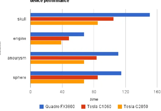
4.1 Algorithm performance running on different devices and with different (small) datasets. . . 47

4.2 Algorithm performance running on different devices and with different (big) datasets. . . 48

4.3 Algorithm speedup running on different devices and with different datasets. 48 4.4 Algorithm device usage on different devices and with different datasets. . 50

4.5 Algorithm components performance on different devices using the skull dataset. . . 51

4.6 Algorithm’s components performance on different devices using the8 skulls dataset. . . 51

4.7 Algorithm’s components performance on different devices using the un-knownHISOdataset. . . 52

4.8 Without prefetch. . . 54

4.9 With Prefetch. . . 55

4.10 Prefetch on OpenCL 1.0. . . 55

4.11 Algorithm components time on different devices using skull dataset. . . . 56

4.12 Algorithm components time on different devices using 8 skulls dataset. . 57

4.13 Algorithm components time on different devices using unknownHISO dataset. 57 4.14 Device usage on different devices and with different datasets. . . 59

4.15 Simple demo test using multiple devices. . . 60

7.1 Skull dataset.. . . 77

7.2 Engine dataset. . . 78

7.3 Aneurysm dataset. . . 78

7.4 Sphere dataset. . . 79

(13)

List of Tables

2.1 Illustration of a naive scan applied to a binary list, resulting in a unique

and sequential values. . . 13

2.2 Illustration of a naive prefix sum applied to a integer list, resulting in the sum of all previous values. . . 13

2.3 Memory allocations and access capabilities. . . 19

3.1 Details about processing a2563 samples dataset using different work unit sizes. . . 27

3.2 Results about processing a2563 samples dataset using different work unit sizes. . . 27

3.3 Details about processing a5123 samples dataset using different work unit sizes. . . 27

3.4 Results about processing a5123 samples dataset using different work unit sizes. . . 29

4.1 Units used in the test results. . . 46

4.2 Datasets used to perform the tests. . . 46

4.3 Systems used to preform the tests. . . 46

4.4 Devices used to preform the tests.. . . 46

4.5 Algorithm performance running on different devices and with different datasets. . . 47

4.6 Algorithm components performance running on a Quadro FX3800 device with different datasets. . . 49

4.7 Algorithm components performance running on a Tesla C1060 device with different datasets. . . 50

4.8 Algorithm components performance running on a Tesla C2050 device with different datasets. . . 50

4.9 Algorithm performance using pinned memory. . . 53

(14)

4.11 Algorithm performance using local memory. . . 53

4.12 Generation component performance using local memory. . . 54

4.13 Algorithm performance using prefetch. . . 54

4.14 Device usage using prefetch.. . . 54

4.15 Algorithm enhanced performance running on different devices and with different datasets. . . 56

4.16 Algorithm’s components performance running on a Quadro FX3800 de-vice with different datasets. . . 58

4.17 Algorithm’s components performance running on a Tesla C1060 device with different datasets. . . 58

4.18 Algorithm’s components performance running on a Tesla C2050 device with different datasets. . . 58

4.19 Algorithm performance using object identification with 2 objects. . . 59

4.20 Algorithm performance using object identification with 65 objects. . . 60

(15)

Listings

6.1 CUDA kernel of matrix multiplication example. . . 67

6.2 CUDA host program of matrix multiplication example. . . 68

6.3 OpenCL kernel of matrix multiplication example. . . 71

(16)

(17)

1

Introduction

Marching Cubes (MC) [LC87] is one of the most common algorithms for indirect volume rendering1_{(IVR) of volumetric datasets, it allows the creation of three-dimensional (3D)}

models of constant value. This can be very useful in many scientific areas, such as med-ical imaging, geophysmed-ical surveying, physics and computational geometry, but some of these applications require huge data sets to produce reliable models. A major problem is that the number of elements grows to the power of three with respect to sample den-sity, and the massive amounts of data puts hard requirements on processing power and memory bandwidth, even harder if the visualization is interactive or dynamic.

In the past, one way of handling problems with massive amounts of data was to use a distributed version2 of the marching cubes algorithm [Mac92]. This approach could use supercomputers or a cluster of computers to speed-up the process, but it yield scale problems due to typical bottlenecks of distributed approaches, like latency and limited bandwidth. More processing units implied more network bandwidth to feed them and a central unit powerful enough to receive the results. Ultimately, to speed-up the process the use of higher frequency CPUs was required, because the overhead of adding more processing units wouldn’t pay-off its costs.

Eventually the increase of frequency stalled and the solution found by the computer industry was to couple more processors in a single physical package. Although the shift

1_{Indirect Rendering techniques involve rendering of an intermediate structure, such as an isosurface, that} has been extracted from the data.

2

(18)

toward multi-core CPU architectures has created a strong potential for highly efficient solutions, at least compared with distributed ones, they still lacked the resources for high demanding usages.

Graphics processing units (GPUs) have always been based on a many-core design and their overall performance has continued to increase at a much higher rate than the tradi-tional multi-core CPUs, shown in figure1.1. Performance increase led to units more pro-grammable, capable of producing complex graphics effects, through the use of shaders3. This also allowed their usage in fields besides graphics applications.

There has been a lot of research on volume data processing using GPUs. This field involves huge computational tasks with challenging memory bandwidth requirements, building on massive parallelism. Such workloads have the potential to preform much better using massive parallel processing devices such as the GPUs, than the highly so-phisticated serial processing offered by the CPUs.

But despite all previous facts, programing GPUs was a lot more complicated and much more restricted than any multi-core CPU architecture.

Figure 1.1:Enlarging peak performance gap between GPUs and CPUs.

With the advent of General-Purpose computing on Graphics Processing Units (GPGPU) came a new degree of freedom to implement algorithms capable of exploiting such pro-cessing power. This would turn GPUs into open architectures, much like the regular CPUs but with tremendous parallel-processing power. To enable this new computing paradigm there are several frameworks, CUDA [NBGS08] introduced by NVIDIA and OpenCL [mun10] proposed by Khronos Group being the most popular ones.

We will be focusing on OpenCL, a new and open standard for task-parallel and data-parallel heterogeneous computing on a variety of modern CPUs, GPUs, DSPs, and other microprocessor designs. This is mainly due to the limited range of hardware devices

3

(19)

supported by other frameworks, they are either limited to a single microprocessor family or don’t support heterogeneous computing. For example, something developed with CUDA can only run on NVIDIA devices.

OpenCL provides easy-to-use abstractions and a set of programming APIs based on past successes with CUDA and other programming frameworks. Even if OpenCL can’t completely hide significant differences in hardware architecture, it does guarantee porta-bility and correctness. This makes it much easier to port OpenCL programs for different architectures, beginning with a generic version and then tweak each of them indepen-dently.

OpenCL can be a significant help in implementing an accelerated version of the March-ing Cubes algorithm. At least compared with graphics-based programMarch-ing standards, al-though much more verbose than similar CPU versions. Besides the advantages from the programming point of view, OpenCL also provides a clean and simple way to manage the hardware resources. A solution that can distribute its workload across several devices has the potential for great performance improvements.

1.1 Motivation

Besides the technical viability, this implementation also seeks its practical use. Its need comes from a scientific project4 that expects to build a set of GPU-accelerated tools. These tools perform heavy computational tasks that without GPU assistance would be too much impractical or require considerable CPU processing power.

Providing a visualization solution like this one using CPU power makes little to no sense. If the final results are presented by the GPU and it’s possible to produce such results using also the GPU, why not do the whole process there?

In situations where it’s practical to use CPU power, the resources can be very expen-sive if similar performances are expected. Using GPU assistance can be viewed as just a way of building a solution that otherwise would be more expensive.

4

(20)

(21)

2

Related Work

In this chapter we provide an introduction to the components used in our solution. Sec-tion2.1 begins with a brief introduction to what are the goals and requirements of the marching cubes algorithm. Then the fundamental stages in the standard algorithm are explained. Ending with some of the relevant approaches to our solution. Section2.2also begins with an introduction, including a brief history of GPGPU and the components of OpenCL. After that, an overview of OpenCL architecture is supplied, described follow-ing four models.

2.1 Marching Cubes

Marching Cubes [LC87] is a computer graphics algorithm, published in the 1987 SIG-GRAPH proceedings by Lorensen and Cline, with the purpose of modeling 3D medical data, typically, produced by scanners such as computed tomography (CT) or magnetic resonance (MR). The output of the algorithm is a polygonal mesh representing points of a constant value (e.g. pressure, temperature, velocity, density) within a volume.

2.1.1 Introduction

Usually we know in advance the shape of the body we want to model, but sometimes that is not the case, therefore, in some of those cases, we can use the marching cubes algorithm to build a close model. To achieve this there are a couple of requirements which are necessary to meet. Anisovaluethat will determine whether a given point is "inside" or "outside" of theisosurface1_{. And a volumetric data set, or a function capable of}

1

(22)

produce such data set, representing the desired model. This data must be arranged as a regularly structured grid of 3D points,P(x, y, z).

2.1.2 Algorithm

The algorithm begins by identifying which is the relevant data to build the isosurface, according to the isovalue specified by the user. This is done analyzing all logical cubes, also known asvoxels2, formed by two adjacent slices of data, each corner has a value, four at each slice, like in figure2.1. Each of these values are compared against a threshold, the isovalue, to determine if it belongs inside or outside the surface, values that exceeds (or equals) the isovalue belong inside. Only cubes with values inside and outside are rele-vant, this means that the surface cuts (intersects) the cube somewhere.

Figure 2.1:Illustration of a logical cube (voxel) formed by two adjacent slices of data.

Since cubes have eight corners and each corner has two possible states, inside and out-side, there are28

= 256possible combinations of edge intersections. In order to simplify the process of determining edge intersections it’s used a look-up table (built offline) with all possible combinations, which is indexed in such way that each corner has a distinct weight, a power of two. For example, if a cube has corner 1 and 3 inside, the correspon-dent index would be 12

+ 32

= 10. In the original MC implementation [LC87] the 256 combinations were reduced to 15, shown in figure2.2, by using symmetry properties like rotation and reflection (complementarity), shown in figure2.3.

Figure 2.2:Illustration of the 15 basic intersection topologies.

Based on the index previously calculated it’s determined which edge topology each relevant cube has, using an edge table (also built offline). Since this table only provides

2

(23)

Figure 2.3:Illustration of reflective (A with Af) and rotational (A with Ar) symmetries.

the intersection topology it’s necessary to calculate the actual intersection based on the value of each corner via linear interpolation. All vertex information needed to build the patches (triangles) that compose the surface is generated in this step.

With all vertex information generated the only thing missing it’s calculating normals for each triangular patch, for smooth rendering purposes. The original algorithm [LC87] calculates a unit normal at each cube vertex using central differences and interpolating the normal for each triangle vertex. Another way [NY06] of accomplish this after the facets have been created is to average the normals of all the faces that share a triangle vertex.

To finish the process it’s necessary to render all vertex information, a collection of triangular patches across all relevant cubes forming the triangular mesh that defines the isosurface. Moreover, the rendering process can also use normal information to produce Gouraud-shaded models.

2.1.3 Challenges

There are two main challenges while using marching cubes algorithm, the first is correct-ness and consistency, the second is efficiency and performance. End-user understanding of a data set is positively impacted if the extracted isosurface is both correct and topologi-cally consistent. An efficient algorithm can also have impact on user experience, specially if the output is a dynamic model and not a static one.

An isosurface is correct if it accurately matches the behaviour of a known function (or some assumed interpolant) that describes the phenomenon sampled in the data set. If each component of an isosurface is continuous then it is topologically consistent. It’s possible for an isosurface to have a consistent topology and not be correct.

(24)

one or both cubes, like in figure2.4(b)and figure2.4(c).

(a) isosurface with holes from an ambiguity in a face shared by two cubes

(b) one alternate facetization that yields a topologically con-sistent isosurface for the cubes

(c) another alternate facetiza-tion that yields a topologically consistent isosurface for the two cubes

Figure 2.4:Illustration of face ambiguity and resolutions.

Since the use of reflective symmetries is what causes face ambiguity, one simple way of resolving the problem directly is to use a look-up table that don’t exploit such symme-tries, like in figure2.5.

Figure 2.5:Illustration the 23 intersection topologies exploiting only rotation.

The facetization of a cube that hasn’t ambiguous faces can still have internal ambigu-ity, this kind of ambiguity doesn’t cause inconsistency but can yield an incorrect isosur-face, as shown in figure2.6.

(25)

(a) disjoint facetizations

(b) linking face-tization

Figure 2.6:Illustration of internal ambiguity (two facetizations of the case 4).

Employing computation avoidance and parallelization techniques can improve the algo-rithm performance.

Beginning with computation avoidance, one way of reducing processing cycles is to avoid unnecessary operations on non-relevant (empty) cells, which in general represents up to 70%. Although this technique can’t be used in all steps, since generating a correct isosurface requires each cell to be visited at least once to determine if the cell is rele-vant or not, it can avoid many unnecessary computations. Another enhancement is the possibility of sharing all common data, from the twelve edges of a cube only three need processing since the rest was already processed or will be, with the exceptions of bound-aries.

Parallelization presents an interesting path for improving performance. In theory a completely parallel algorithm can lead to unlimited speed-ups, with the necessary re-sources. Like most graphics algorithms, marching cubes exhibits a degree of intrinsic parallelism (e.g., cube faces not shared with previously visited cubes can be processed independently), its parallelization offers the potential for performance improvement.

Sometimes there are commitments between efficiency and performance that need to be done. A parallelized solution of marching cubes requires splitting data to be dis-tributed through the processing resources, and each portion of data has boundaries that are shared with adjacent portions. This means that some data is duplicated, wasting memory, and some work is also duplicated, wasting processing cycles. Typically, this kind of commitments have a spot where efficiency and performance are better combined.

2.1.4 Implementations

(26)

complexity of such solutions, mostly due to programming functionality being graphics-based.

Prior to the introduction of geometry shaders (GS), GPUs completely lacked function-ality to create custom primitives directly. Consequently, geometry had to be instantiated by the CPU or be prepared as a vertex buffer object (VBO). Therefore, a significant part of the work needed to be done in the CPU. Or a fixed number of triangles had to be as-sumed for each MC cell, wasting unnecessary resources.

A very common approach while using vertex shader (VS) or fragment shader (FS) so-lutions is to exploit a generalization of the MC algorithm, the marching tetrahedra (MT) algorithm [Elv92]. It has some advantages due to the reduced amount of redundant tri-angle geometry, since MT never requires more than two tritri-angles per tetrahedron. In addition, inspecting only four corners is enough to determine the configuration of the tetrahedron, reducing the amount of inputs. MT has also the advantage of being easily adapted to unstructured grids. Pascucciet al.[Pas04] and Kleinet al.[KSE04] are a couple of examples that explored this approach.

Even though MT being very common there are also approaches that used the MC algorithm. Goetz et al. [KW05] used the CPU to classify MC cells and only then were passed to the GPU to process the rest of the algorithm. A similar approach was followed by Johanssonet al.[JC06] where a kd-tree were used to cull empty regions. In both situa-tions was noted that this pre-processing on the CPU limits the speed of the algorithm.

When using hardware with shader model (SM) 4 capabilities the GS stage can pro-duce and also discard geometry on the fly. This is very useful since most methods based on previous hardware generations produce isosurfaces that are cluttered with degener-ate geometry. Degenerdegener-ated geometry can yield poor performance because of unneces-sary computations, which can represent a significant percentage. To produce a compact sequence of triangles additional post-processing is required, such as stream compaction.

(27)

unnecessary copy of data.

Another implementation of MC in CUDA is presented by Nagel [Nag08]. This ap-proach has very specific properties, it’s able to handle data sets so large that cannot be entirely loaded in the working computer’s main memory. These data sets can be of two kinds, a single volumetric grid that is too large to fit in memory and many temporal volumetric grids that individually fit in memory, but combined don’t. Because of these restrictions the process is force to compute only data set’s portions at a time in the GPU and then send them back to the CPU. After that, vertex information is compressed to make rendering possible. Thanks to this method the author claims that this solution can handle data sets as large as 77GB.

The NVIDIA GPU Computing SDK also provides an MC implementation in CUDA C source form3. Because of that it will be provided a deeper presentation than previously done with other presented solutions. Although, trying to omit certain implementation details or optional features for simplicity sake. Even without any kind of introduction to NVIDIA’s CUDA framework shouldn’t be too difficult to understand the implemen-tation principles. Besides, most framework architecture details are common to OpenCL, examined in the section2.2.

The application follows a typical structure of a GPGPU approach. It’s composed of two parts, the main program that executes on the CPU and functions that execute on the GPU.

The main program executed on the CPU do initializations, memory allocations and CUDA device coordination. All code that is executed only once or just a few times, work where serial processors are good at. The source code file ismarchingCubes.cppand most relevant functionality is in functioncomputeIsosurface().

The functions executed on the GPU do all operations that require large amounts of iterations and can be parallelized. These programs represent, or at least should represent, all the heavy work and most of the processing cycles.

The source code file ismarchingCubes_kernel.cu.

The application has three functions that run on the GPU, each with a different task:

1. classification of voxels topology (classifyVoxel)

2. separation of occupied voxels from empty ones (compactVoxels)

3. calculation of triangle’s vertices and normals (generateTriangles)

Additionally, there’s also a CUDPP library4 function that runs on the GPU, preforming scan operations, also known as perfix sum operations. All these functions will be further explained in the algorithm context.

(28)

One relevant part of the MC algorithm is the look-up table, which in this case is built offline and stored like a texture. In this solution there’s also a vertex table that covers all possible cube topologies, also built offline and stored like a texture. Since the data being processed is arranged in a 3D form, the processing elements are also organized in such way. All other bits of initialization, memory allocation, and other operations which aren’t relevant to the MC algorithm will be ignored.

This MC algorithm begins by classifying all voxels in the data set, this operation is done by the first GPU function. The goal of this evaluation is to populate two lists, one with the numbers of vertices per voxel, the other indicating whether a voxel is occupied. Each thread processes one voxel at a time and regardless its organization all vertex are verified, even if some vertices are shared with other voxels.

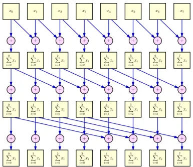
After classification an scan operation (also known as prefix-sum) is applied on the binary list that contains all occupied and empty voxels. A naive version of this operation is able to sumnelements of a list inlog2(n)steps, illustrated in figure 2.7. Along with

the sum, it also produces a new list where all ones are replaced by unique and sequential values, as shown in table2.1.

Figure 2.7:Illustration of a naive scan applied to an eight-element list inlog2(8) = 3steps.

(29)

1 0 0 1 1 0 1 1 1 1 0 1 2 1 1 2 1 1 1 2 2 2 3 3

1 1 1 2 3 3 4 5

Table 2.1:Illustration of a naive scan applied to a binary list, resulting in a unique and sequential values.

After compaction another scan operation is applied, this time on the list containing the vertices for each voxel. The operation results in its sum and a list that contains the vertices index for each voxel. The principle is the same as the above but with integers, shown in table2.2.

3 0 0 6 3 0 9 12

3 3 0 6 9 3 9 21

3 3 3 9 9 9 18 24 3 3 3 9 12 12 21 33

Table 2.2:Illustration of a naive prefix sum applied to a integer list, resulting in the sum of all previous values.

All previous stages produced the necessary information for starting the triangle gen-eration at this stage, it corresponds to the third GPU function. Vertices are interpolated to find out where the actual edge intersection occurred, producing more detail. This in-formation is stored in shared memory instead of local one, which is claimed to be faster. After that, it starts organizing vertices in triangles, and calculating their surface normals. The final result is the population of two lists, one with vertex information, the other with normal information. The information of these two lists are indexed based on the list produced in the previous stage, creating a compact stream of isosurface triangles. Since there’s a list of occupied voxels it’s possible to run this operation only on them, discard-ing all irrelevant ones.

The final stage is rendering all triangle information to create the isosurface. Addition-ally, the triangle surface normal information is used to enable shading.

Besides some brute force operations, like the verification of voxels topology, all heavy work is done in GPU, ensuring good performance and even interactivity. One detail that is also pointed in the source code is that, it’s possible to combine the both scan operations into just one. Because the information related with each voxel shares the same index in both lists.

(30)

easy to understand. The scan operation used was inclusive when in reality the exclusive is used, it fits computer programming needs better. In the exclusive prefix sum, the first element in the result list is the identity element (0 for add operation) and the last element of the operand list is not used. More detailed information about these operations with CUDA is available in [HSO07].

(31)

2.2 OpenCL

OpenCL (Open Computing Language) is an open royalty-free standard for general pur-pose parallel programming across CPUs, GPUs and other processors, giving software developers portable and efficient access to the power of these heterogeneous processing platforms.

2.2.1 Introduction

The internal architecture of early GPUs were too tied to graphics programming stan-dards such as DirectX and OpenGL. The tight relationship ensured an overall good per-formance, but limited the possibilities to what was provided by such graphics standards. Eventually, the GPU makers introduced customizable processing elements in the GPUs pipelines to overcome this limitation. These elements were able to run specific programs, called shaders.

Custom processing elements evolved over time, replacing more fixed function stages in the GPU pipeline. Eventually all these elements were unified, being able to provide functionality that were previously offered by different elements. The change was also reflected in the shaders, that went from assembly to high-level languages, capable of of-fering programs with advanced functionality. This would allow the creation of stunning applications, like video games, and the beginning of what is today known as GPGPU.

Before the introduction of GPGPU standard APIs this kind of processing was already done, it could be accomplished using OpenGL and DirectX APIs, but that was a really tough job.

When Nvidia introduced its GPGPU implementation, known as CUDA, the task of creating something capable of running on a GPU became much easier. This framework provides an easy API, which isn’t graphics-based like OpenGL or DirectX, coupled with C language (with some restrictions and Nvidia extensions) for writing kernels, the actual functions that execute on GPU devices.

OpenCL born from efforts of Apple while developing the Grand Central framework, its goal was to make multi-threaded parallel programming easier, later they realized it could be mapped nicely to the GPGPU problem domain. Then they wrapped up their Grand Central API into an API specification and, supported by Nvidia, AMD and Intel, released it to the Khronos Group as OpenCL.

(32)

The language specification describes the syntax and programming interface for de-veloping kernels. The language used is based on subset of ISO C99, due to its prevalence and familiarity in the developer community. To guarantee consistent results across dif-ferent platforms, a well-defined IEEE 754 numerical accuracy is defined for all floating point operations. One of the weakest points in CUDA is not being able to guarantee such accuracy, very important in scientific fields. There’s also some functions that assist the manipulation of such numerical formats. The developer has the option of pre-compiling their OpenCL kernels or letting that operation be preformed in runtime. Compilation in runtime guarantees that kernel programs can run on devices that don’t even exist.

The platform layer API offers access to functions that query the OpenCL system, pro-viding all kinds of useful information. Based on such information, developers can then choose the fittest compute devices to properly run their workload. It is at this layer that contexts and queues for operations such as job submission and data transfer requests are created.

The runtime API is responsible for managing the resources in the OpenCL system. It allows performing operations defined in contexts and queues.

2.2.2 Architecture

To help describe OpenCL architecture, it’s presented a hierarchy of models based on OpenCL specification [mun10]:

• Platform Model

• Memory Model

• Execution Model

• Programming Model

2.2.2.1 Platform Model

Every OpenCL environment has onehost, where the software to control the devices is ex-ecuted, typically a CPU. The host is connected to, at least, onecomputational device, which can be a CPU, GPU, or another accelerator. Each device contain one or more compute units(processor cores). And these units are themselves composed of one or more single-instruction multiple-data (SIMD)processing elements. This model is shown in figure2.8.

2.2.2.2 Execution Model

(33)

Figure 2.8:Illustration of the platform model.

devices.

The key property of OpenCL execution model is defined by how kernels execute. Each kernel submitted for execution gets an index space, which is mapped to all in-stances. A kernel instance is called work-item and is identified by its index in the cor-responding index space. The kernel code executed is the same in all work-items but each one of them has a different identification (ID), allowing different execution pathways.

Each kernel submission is applied to a group of work-items, calledwork-group. These groups provide a simple yet powerful organization and like work-items they are also identified by an index. Since work-items IDs are only unique within a work-group it’s necessary to use their global ID or a combination of their work-item and work-group IDs to identify them globally. The work-items in a given work-group execute concurrently on the processing elements of a single compute unit.

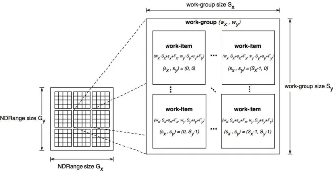
The space index used to identify work-items or work-groups is called NDRange. A NDRange is an N-dimensional index space, where N can be one, two or three. Figure2.9 is an example of a two-dimensional (2D) arrangement of work-groups and work-items.

After learning how working units are organized it’s time to know how to submit re-quests to them. OpenCL defines acontextthat provides resources to enable the execution of the kernels. The context includes the following resources:

Devices The collection of OpenCL devices to be used by the host.

Kernels The OpenCL functions that run on OpenCL devices.

Program Objects The program source and executable that implement the kernels.

(34)

Figure 2.9:Illustration of a two-dimensional (2D) arrangement of work-groups and work-items.

OpenCL API provides functionality to create and manipulate the context. To coor-dinate the execution of the kernels there’s a facility called command-queue. This queue schedules commands onto the devices within the context. These commands include the following functionality:

Kernel execution commands Execute a kernel on the processing elements of a device.

Memory commands Transfer data to, from, or between memory objects, or map and unmap memory objects from the host address space.

Synchronization commands Constrain the order of execution of commands.

The commands queued are then executed asynchronously between the host and the device. The order of execution depends on the mode, which can bein-orderorout-of-order. In-order execution guarantees the submission order. It fallows the logic first in first out (FIFO), in other words, a prior command on the queue completes before the following command begins. This serializes the execution order of commands in a queue.

Out-of-order execution doesn’t enforce any particular order, following commands don’t have to wait for the current to finish execution. Any order constrains must be enforced by the programmer through explicit synchronization commands.

(35)

It is possible to associate multiple queues with a single context. These queues run con-currently and independently with no explicit mechanisms within OpenCL to synchronize between them.

2.2.2.3 Memory Model

OpenCL defines four different memory regions that are available to the kernels. These memory regions differ mainly in size, latency and access capabilities. Much like the lev-els of cache in a CPU, with the exception that in OpenCL they are explicitly manipulated, providing great potential for optimizations. Smaller regions are the fastest and also clos-est to the working units, and vice-versa. A conceptual OpenCL device memory model is shown in figure2.10. Table2.3resumes memory allocations and access capabilities of different regions from the device and the host.

Global Memory This memory region permits read/write access to all work-items in all work-groups. Work-items can read from or write to any element of a memory ob-ject. Reads and writes to global memory may be cached depending on the capabil-ities of the device.

Constant Memory This memory region permits read access to all items in all work-groups. Work-items can read from or write to any element of a memory object. Reads and writes to constant memory may be cached depending on the capabilities of the device.

Local Memory A memory region local to a work-group. This memory region can be used to allocate variables that are shared by all work-items in that work-group. It may be implemented as dedicated regions of memory on the OpenCL device. Alternatively, the local memory region may be mapped onto sections of the global memory.

Private Memory A region of memory private to a work-item. Variables defined in one work-item’s private memory are not visible to another work-item.

Global Constant Local Private

Host Dynamic allocation Dynamic allocation Dynamic allocation No allocation

Read / Write access Read / Write access No access No access

Device No allocation Static allocation Static allocation Static allocation

Read / Write access Read-only access Read / Write access Read / Write access

Table 2.3:Memory allocations and access capabilities.

(36)

Figure 2.10:Illustration of a conceptual OpenCL device memory model.

copying data or mapping and unmapping regions of a memory object. These two opera-tion are accomplished using the command queuing mechanism explained previously, in sub-sub section2.2.2.2.

Explicit copy of data between the host and a device may be a blocking or non-blocking operation. Blocking operation function calls return only after the host can be safely reused, without the risk of tempering the data being transferred. Non-blocking opera-tion funcopera-tion calls return as soon as the command is enqueued.

OpenCL uses a relaxed consistency memory model, for example, the state of memory visible to a item is not guaranteed to be consistent across the collection of work-items at all times.

Within a work-item memory has load / store consistency. Local memory is consistent across work-items in a single work-group at a work-group barrier. Global memory is consistent across work-items in a single work-group at a work-group barrier, but there are no guarantees of memory consistency between different work-groups executing a kernel.

2.2.2.4 Programming Model

(37)

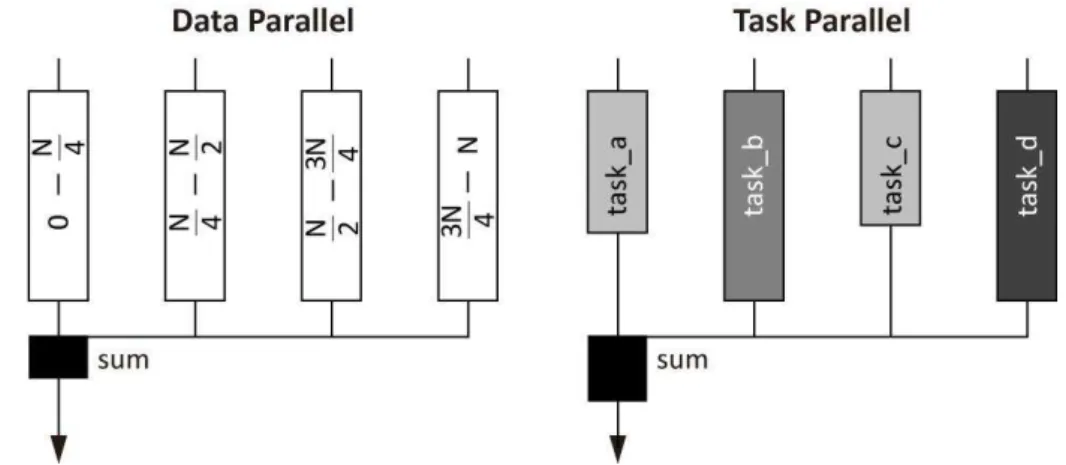
In the data parallel programming model, the same kernel is passed through the com-mand queue to be executed simultaneously across the compute units or processing ele-ments. The index space associated with the OpenCL execution model defines the work-items and how the data maps onto the work-work-items.

For the task parallel programming model, different kernels are passed through the command queue to be executed on different compute units or processing elements. The parallelism can be express by enqueuing multiple tasks.

The figure 2.11shows the different between the two models. Supposing that a pro-gram is composed by four independent tasks that operate on a data set to produce a result. While it’s possible to process those four tasks simultaneously it’s also possible to divide the data in four equal parts and apply the combination of the four tasks to them simultaneously.

Figure 2.11:Illustration of the difference between data parallel and task parallel programming models.

There are two domains of synchronization in OpenCL, items in a single work-group and commands enqueued to command-queue(s) in a single context.

Synchronization between work-items in a single work-group can be accomplished us-ingbarriers. All the work-items of a work-group must execute the barrier before any are allowed to continue execution beyond the barrier. Note that the work-group barrier must be executed by all work-items of a work-group or by none of them, to avoid dead-locks. There is no mechanism for synchronization between work-groups.

Synchronization between commands in command-queues can be accomplished using

barriersorevents.

(38)

(39)

3

Implementation

3.1 Introduction

The goal is to implement an (indirect) volume rendering solution using the Marching Cubes algorithm, taking advantage of the OpenCL framework. This framework allows to accelerate the execution of the algorithm, using heterogeneous processing devices, in its heavy paths. Which means that besides the traditional CPUs it’s possible to use GPUs and other kinds of (parallel) processors, like the IBM Cell, to explore their high paral-lel processing power. Also, this framework is device/vendor independent (contrary to CUDA), it provides portability between different families of devices. The implementa-tion tries to be as efficient and parallel as possible, allowing it to be fast and scale up well in multi-processor devices. Its generic design tries to promote extensibility and readabil-ity over small tweaks.

3.2 Summary

This implementation bundles two important components, one focused on the Marching Cubes algorithm (mc* prefixed modules) and the other addressing OpenCL implementa-tion details (cl* prefixed modules). The algorithm component has two fundamental mod-ules, one in charge of decompose and distribute the work for the available processing devices (mcDispatcher) and the other containing a Marching Cubes algorithm’s imple-mentation (mcCore). The OpenCL component part offers extended functionality (clScan) and low-level API abstraction (clHelper).

(40)

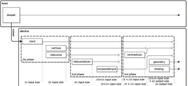
for the available processing devices, following a method similar to round-robin. This division of the dataset in smaller pieces allows big volumes of data to be processed, in addition to enable the usage of more than one device in parallel. These work units are computed by the mcCore module, which can work in parallel by (at least) as many in-stances as available devices, each producing a fraction of the output until all of them are finished. The mcCore implementation of the Marching Cubes algorithm takes as input an isovalue and a dataset and outputs the corresponding 3D model (geometry and shad-ing). This module is divided in three phases (classification, compaction and generation), closely corresponding the three OpenCL kernel functions used to speed up the algorithm.

Figure 3.1: Overview of the execution work-flow (to keep it simple only Marching Cube modules are visible, most OpenCL modules usage is done inside mcCore module).

3.3 Host Modules

3.3.1 mcDispatcher

This module divides the work into smaller pieces, called work units, and dispatches them to be processed. Each work unit produces a memory entry (a fraction of the final result) that make the output list. The division of work brings some advantages, related to a higher division granularity, but there are also some associated costs.

One important advantage is the possibility of processing high quantities of data (big datasets). The memory usage during a regular execution of the algorithm (mcCore mod-ule) reaches several times the input (dataset) size, without the division it would be im-possible to process an input with more than a small fraction of the device’s memory.

(41)

way, each has an independent execution path (using threads) and it’s responsible for requesting work every time it becomes unoccupied and there’s available work units yet to be processed.

The associated costs of duplicate data across boundaries of two consecutive work items are seen as overhead. Since datasets and work units are made of slices (like a stack of paper), being one slice (a sheet) the smallest unit of data, each division accounts for (at least) one slice of overhead. In addition, the process of dispatching may have to account for exceptions, boundaries that didn’t result from division (the first and last slice) require especial treatment. This exceptional treatment only happens when the duplicated data goes further behind the boundary, in such case the overhead grows up one slice, in both extremities (exception made to the the first and last slice), for each extra level of duplicity. Another technical detail that influences the overhead is the work unit size, it must be defined considering aspects like overhead ratio, runtime algorithm’s memory requirements, fair distribution of work across multiple devices, among others.

Besides the resulting overhead there’s also the extra technical work of coordinate mul-tiple concurrent paths of execution (threads). This coordination make use of locks, a mu-tual exclusion method, to ensure that each work unit (or some part of it) is assigned only to one device. A central variable is used to hold the progress of work, it points to the first slice of the remaining undone work. Whenever a work unit is requested this variable is updated to reflect the current progress of work, in a complete exclusive way.

Figure 3.2:mcDispatcher module execution work-flow.

3.3.1.1 Work Unit Size

(42)

As previously mentioned, during a regular execution of the algorithm (mcCore mod-ule) the memory usage reaches several times the input (work unit) size, which can be-come a problem if the input size is too big. In extreme cases can be impossible to run a single execution the algorithm, in less extreme cases there’s still the problem of the lim-ited amount of space to store other work units results (algorithm runtime needs + other work units results). Another issue with big work units is the unbalanced distribution of work when using multiple devices, specially relevant on the last work units. Some devices may become idle whereas others stay running for a significant period of time.

While using big work units leads to unwanted consequences, using too small units also has big disadvantages. Small work units means more divisions, more duplicated data, more overhead and a bigger performance hit. This happens because duplication is done for complete slices, so even if each slice is quite big (its area) but the work unit has just a few of them the overhead is high.

Device processing power can also assist the decision, specially useful when there are multiple devices and they yield different performances. Although useful in certain situa-tions this subject wasn’t deeply studied and because of that it doesn’t help in the decision making process.

To see how the work unit size affects the algorithm’s execution some tests were con-ducted using two different sized datasets,2563

and5123

samples, while different work unit sizes are being used. To focus the attention on this subject and keep things as simple as possible no additional details will be given about the input or the output, they are not important here and are further analysed in chapter 4. This results help choose a good work unit size in ideal conditions.

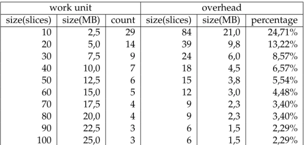
Tables3.1and3.3present details about the execution, the columnssizeandpercentage

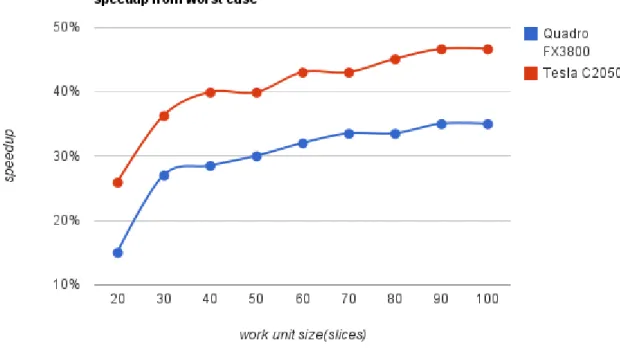
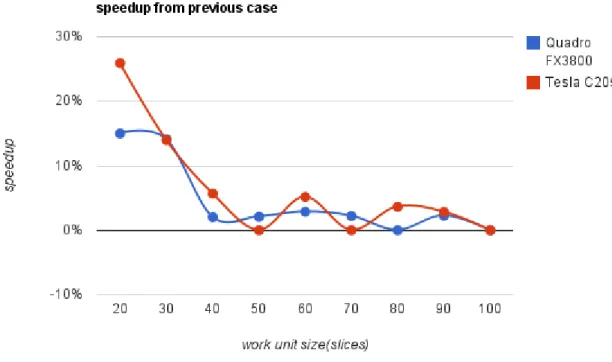
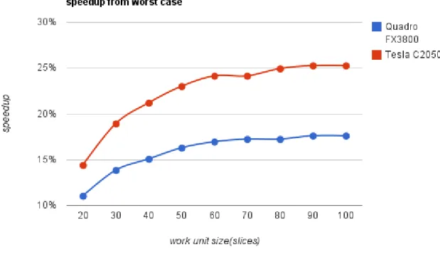
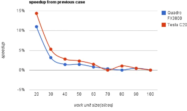
are pretty much self explanatory and the column counthas the quantity of work units resulted from the corresponding work unit size. Tables3.2and3.4present results about the execution, the columns time have the total time spent, the columns worst have the speedup (in percentage) from the worst case (which is the first), the columnsprevioushave the speedup (also in percentage) from the previous case (hence the non existing result in the first case) and the column speedup has the speedup between the devices. Figures 3.3,3.4and3.5 are charts based on the results from table3.2(2563

samples dataset) and figures3.6,3.7and3.8are based on the table3.4(5123

samples dataset).

(43)

work unit overhead

size(slices) size(MB) count size(slices) size(MB) percentage

10 2,5 29 84 21,0 24,71%

20 5,0 14 39 9,8 13,22%

30 7,5 9 24 6,0 8,57%

40 10,0 7 18 4,5 6,57%

50 12,5 6 15 3,8 5,54%

60 15,0 5 12 3,0 4,48%

70 17,5 4 9 2,3 3,40%

80 20,0 4 9 2,3 3,40%

90 22,5 3 6 1,5 2,29%

100 25,0 3 6 1,5 2,29%

Table 3.1:Details about processing a2563

samples dataset using different work unit sizes.

work unit Quadro FX3800 Tesla C2050

size(slices) time(ms) worst previous time(ms) worst previous speedup

10 200 - - 193 - - 1,04

20 170 15,00% 15,00% 143 25,91% 25,91% 1,19

30 146 27,00% 14,12% 123 36,27% 13,99% 1,19

40 143 28,50% 2,05% 116 39,90% 5,69% 1,23

50 140 30,00% 2,10% 116 39,90% 0,00% 1,21

60 136 32,00% 2,86% 110 43,01% 5,17% 1,24

70 133 33,50% 2,21% 110 43,01% 0,00% 1,21

80 133 33,50% 0,00% 106 45,08% 3,64% 1,25

90 130 35,00% 2,26% 103 46,63% 2,83% 1,26

100 130 35,00% 0,00% 103 46,63% 0,00% 1,26

Table 3.2:Results about processing a2563

work unit overhead

size(slices) size(MB) count size(slices) size(MB) percentage

10 10 57 168 168 24,71%

20 20 27 78 78 13,22%

30 30 18 51 51 9,06%

40 40 14 39 39 7,08%

50 50 11 30 30 5,54%

60 60 9 24 24 4,48%

70 70 8 21 21 3,94%

80 80 7 18 18 3,40%

90 90 6 15 15 2,85%

100 100 6 15 15 2,85%

Table 3.3:Details about processing a5123

(44)

Figure 3.3:Processing time of a2563

Figure 3.4:Processing speedup from worst case of a2563

(45)

Figure 3.5:Processing speedup from previous case of a2563

work unit Quadro FX3800 Tesla C2050

size(slices) time(ms) worst previous time(ms) worst previous speedup

10 1063 - - 883 - - 1,20

20 946 11,01% 11,01% 756 14,38% 14,38% 1,25

30 916 13,83% 3,17% 716 18,91% 5,29% 1,28

40 903 15,05% 1,42% 696 21,18% 2,79% 1,30

50 890 16,27% 1,44% 680 22,99% 2,30% 1,31

60 883 16,93% 0,79% 670 24,12% 1,47% 1,32

70 880 17,22% 0,34% 670 24,12% 0,00% 1,31

80 880 17,22% 0,00% 663 24,92% 1,04% 1,33

90 876 17,59% 0,45% 660 25,25% 0,45% 1,33

100 876 17,59% 0,00% 660 25,25% 0,00% 1,33

Table 3.4:Results about processing a5123

(46)

Figure 3.6:Processing time of a5123

Figure 3.7:Processing speedup from worst case of a5123

(47)

Figure 3.8:Processing speedup from previous case of a5123

slices it’s a better approach than using the storage space.

Even with 30 being a good choice there are some situations where this size is not practical, specially when dealing with big slices (its area). Since it’s important to keep a moderate usage of memory because of the runtime needs and the results from other work units, the storage space approach is also used to limit extreme cases. This implies an enforcement of maximum and minimum limits in the memory usage, based on the device memory and reference dataset sizes. Besides device memory, dataset sizes are also used because they provide real numbers. As reference datasets, the small one has

1283

samples (8MB) and the big one has10243

samples (4GB). The minimum work unit size is set to 4MB, which allows the small dataset to be divided in 2 work units (each with 64 slices). The maximum work unit size is set to the smaller size between 128MB or

(48)

3.3.2 mcCore

As previously mentioned, this module contains the Marching Cubes algorithm imple-mentation and it’s divided in three phases. In fact, the first two phases are just an effi-ciency requirement due to parallel implementation constrains, that is, the third (and last) phase do all the necessary work to build a model from the input dataset. The first two phases are just responsible for analyse and discard all the irrelevant data, generating a compacted version of the input dataset. This way the third phase will only process data that matters, and since it’s the most expensive, the two previous phases are very im-portant in the whole process. Previous implementations of the algorithm using OpenGL without Geometry Shaders suffer a great performance hit because weren’t able to discard useless data, this would consume too much memory and processing time, render them inefficient and unable to scale up.

All critical paths of the algorithm are executed making use of OpenCL, through kernel functions. The host code provides the glue for setting up the execution of the algorithm, making a pipeline with the three phases.

The execution (and the first phase) begins by uploading the input dataset data to the device memory (in 3D texture form) and creating the two necessary memory buffers to output the results from the mcClassification kernel. These memory buffers, filled by the execution of the kernel, contain the analysis of the dataset (according to the chosen iso-value). For each voxel, one buffer indicates if the voxel is relevant (occupied) or not and the other the voxel’s number of vertices (or triangles). The relevance buffer may seem redundant, since it is possible to deduce it from the buffer with the number of triangles (it’s only relevant if it has at least one triangle), but is necessary for the next phase. The execution of the kernel ends this phase.

(49)

the second phase.

The third and final phase is responsible for producing the model’s geometry and the corresponding shading data. The result are two buffers, one containing groups of three vertices (triangles) and the other their normals, filled by the mcGeneration kernel. But before executing it there’s one thing missing, a scanned version of the buffer with the amount of vertices per voxel (produced in the first phase). The result is a buffer with unique indexes (or positions) for all relevant voxels, but this time not sequentially or-dered (non-binary array). Each index is the sum of the vertices from all previous entries. This fulfils exactly the requested needs because it allows to output all data in independent positions (addresses) and without any holes, similar to what was done in the previous phase. And once again, the sum of all entries, preformed by the scan, is useful to deter-mine the output buffers size. After being scanned the triangles buffer is released since it’s no longer needed. Now it’s possible to execute mcGeneration kernel, which fills the output buffers. At this point, all remaining buffers, except the last two (geometry and shading buffers), are released and the algorithm is finished.

Figure 3.9:mcCore module execution work-flow.

3.3.2.1 Memory Usage

(50)

Figure 3.10:mcCore module memory usage.

3.3.2.2 Data Format

This module takes as input a dataset and an isovalue, both of which are floating-point type (cl_float). The dataset is a simple array, implicitly arranged in a three dimensional form (volume’s data), and the isovalue is a single value. The output can be released in one of two forms, VBOs1_{or OpenCL memory buffers, these are also floating-point type}

(cl_float4) and are stored in device memory. The difference between the two is that only memory buffers can be retrieved by the host and only VBOs can be used directly by OpenGL.

3.3.2.3 CPU Implementation

A serial implementation that resembles the OpenCL one but skipping the unnecessary tasks, like compaction and all involved steps. Such implementation has the purpose of being the base reference for a serial version, it’s very important to see how the OpenCL implementation preforms against it. The followed approach was to build something that could provide the same results while making it very simple and clean. Although it has no special tweak, the execution path is very strait forward which make it very fast.

The results aren’t uploaded to the GPU, which isn’t completely fair when compared with the OpenCL implementation.

3.3.3 clScan

This module provides thescanoperation, a fundamental functionality in this implemen-tation, also known asprefix sumorreduction. The operation outcome is the sum of all val-ues from a vector while arranging it in a very useful way, performed in parallel, which makes such operation a very important piece of parallel computation.

(51)

Just to recap, each value in the output vector results from summing all previous val-ues in the input vector (e.g.: out[2] = in[0] +in[1]). This operation has two variants,

inclusive 2 and exclusive 3, the former sums all previous values including it self while the latter doesn’t, only includes previous values. While there are two variants, only the exclusive one is relevant in this case because its values can be used as proper indexes.

The output values can be used to uniquely address their corresponding4input ones, that is, for each non-null input value there’s a corresponding unique output one. These values can be used as unique addresses to define independent and self-contained chunks of data on shared resources, allowing multiple processor units to operate simultaneously on it.

In this implementation scan is used to know the output size and the output indexes of dynamic sized buffers. The first case uses the scan operation on a binary vector, which counts (summing just ones and zeros can be thought as counting) how many elements (or components) are non-null and at the same time produces a vector containing unique and sequential indexes just in the corresponding non-null elements positions. These results are used to create a vector containing only non-null data based on the previous binary input vector. The second case uses scan on an integer vector, which sums all its elements and indexes (not sequentially) the non-null ones. Such results are used to create buffers and define independent chunks of data within them.

This module reuses theOpenCL Parallel Prefix Sum (aka Scan) Example5

from Apple, adapted to fit the needs of the implementation. Instead of creating it from scratch the solution was forked from Apple’s example, which provides features like non-power of two sizes, memory bank conflict avoidance and usage of local memory to store partial sums.

3.3.4 clHelper

This module provides some abstractions to the low-level OpenCL API. Tasks such as er-ror reporting, resource and program handling, resource information, profiling and some others are offered as simple functions. Such tasks would require several steps using the OpenCL API. These functions try to be as generic as possible although some of them make some compromises oriented towards this implementation. This abstracted API was created with usability in mind, properties like similar behaviour and ease of use show that.

Although errors can be ignored, all functions handle and forward OpenCL errors, which can be very useful to know how things go in the OpenCL runtime while still using these abstractions.

2_e.g:_out_{[1] =}_in_{[0] +}_in_[1] 3_e.g.:_out_{[1] =}_in_[0]

4_{the same position in both vectors}

(52)

Some functions return the result directly instead of changing the arguments’ refer-enced value, a very common approach in the OpenCL API. Tasks returning data in na-tive types can be greatly simplified, reducing to just a function call what would require several lines of code using the OpenCL API. Profiling, resource information and error reporting functions benefit most with such approach.

Management of resources allows to initialize and free OpenCL resources in one step each, tasks that can be highly automatized. This is mostly because these resources are the minimum requisites to preform any useful work using OpenCL. Besides the common steps to initialize such resources, like platform and device selection and assignment of command queues to devices, the context creation also handles interoperation between OpenCL and OpenGL. Platforms can be selected based on their name, devices can be se-lected based on a provided list and their type. The creation returns a (struct) object that comprises the necessary OpenCL (opaque) objects, while the first is used by some func-tions offered by this module it’s still possible to have direct access to OpenCL using the second ones. Besides the necessary OpenCL objects there’s also some useful information, which avoids querying OpenCL to know things like the maximum work-group size and available global and local memory.

Compilation and management of binaries are handled in a simple and automated manner. It’s possible to compile programs’ sources into binaries and store them on disk for future use. This avoids compiling always from source, which shrinks the initialization process time.

Simpler functionality such as resources information, error reporting, profiling events and creating shared buffers (GL-CL) are also provided.

3.4 OpenCL

3.4.1 Kernels

3.4.1.1 mcClassification

This kernel is responsible for analyse and classify all voxels from the input dataset. This work depends on the isovalue, it influences the interpretation. The result is the output of two arrays – one containing relevance (occupied or empty, binary values) the other vertices, for each voxel.

(53)

grid, it follows closely the input dataset form (3D texture) to avoid unnecessary con-versions between different arrangements (1D to 3D). Although useful it’s not strictly re-quired, instead of calculating only the output position (on 1D arrays) it would be possible to use an 1D arrangement of work-items and calculate the necessary coordinates (on a 3D texture) instead. But since most operations are related to the input it’s much preferable to use 3D arrangement of work-items. Later kernels will not follow this approach be-cause in those situations it would be counter productive, further details about them will be given ahead.

The execution can be started as soon as the dataset and the isovalue are available (and the output arrays are created). Each work-item gets its own coordinates, the base to determine the voxel’s corners coordinates used to read the corresponding values from the input texture. Together with the isovalue these corner values are used to determine the voxel’s combination, which is then used to know how many vertices (or triangles) the voxel will produce. To know how many vertices a combination produces there are a table with all possible combinations (256) that are looked up, this table was built offline. Since the output is done to an unidimensional array, it’s necessary to convert a 3D position to an 1D position. The 1D position is then used to write the amount of vertices and its binary variant (relevance - has vertices or not), to each array.

Kernel 1mcClassification pseudo-code

input:dataset, isoValue

output:occupied[], vertices[]

sizes←getSizes()

coordinates←getCoordinates()

outputP osition←getP osition(coodinates, sizes)

corners[8]←getV oxelCornersV aluesF romDataset(dataset, coordinates)

combination←calculateV oxelCombination(isoV alue, corners)

verticesCount←getV oxelV erticesCount(combination)

vertices[outputP osition]←verticesCount

ifverticesCountthen

occupied[outputP osition]←OCCU P IED_V OXEL

else

occupied[outputP osition]←EM P T Y_V OXEL

end if

3.4.1.2 mcCompaction

(54)

than one thread of execution problems arise, some data paths may suffer from concur-rency problems, in particular the output positions. To solve such problems it’s common to use a mutual exclusion method to protect the affected data, but such technique doesn’t fit well under our model of independent data, it greatly hits parallel performance. A bet-ter solution to this problem can be achieved with an extra array, holding the positions for all output data, which can be obtained by a scanned version of the input array. Note that this result can only be accomplished in arrays with binary values, which is the case (when needed, convert non-binary arrays to binary ones can be easily done). With the positions (addresses) for all output entries obtained, each work-item will be in charge of processing one entry, and since all entries are independent it’s possible to process all of them in a truly parallel way.

Once again there’s a direct relation between the input data size and the amount of work-items launched (1:1), but not with the output data size. In contrast with the previ-ous kernel, this doesn’t arrange work-items in a 3D grid, it prefers a flat 1D arrangement because all data arrays involved (the inputs and the output) are unidimensional.

Each work-item begins by getting its index, which uses to determine the entry it’s in charge with and where it can write the results (through the scanned array). Then, it only has to check the corresponding input value to decide if it has to write its index to the output array or not.

This kernel doesn’t perform compactionper se, it only discards data considered irrel-evant, producing (in general) a much smaller array, hence the name.

Kernel 2mcCompaction pseudo-code

input:values[], scannedValues[]

output:compacted[]

position←getP osition()

compactedP osition←scannedV alues[position]

ifvalues[position]then

compacted[compactedP osition]←position

end if

3.4.1.3 mcGeneration

The last kernel is responsible for producing all model’s data (geometry and shading). It takes as input a dataset, an isovalue, a scanned version of the array containing the amount of vertices each voxel produces and an array holding only the indexes of the voxels which produce vertices (relevant ones), referred to as compacted. And outputs two arrays, these contain geometry (vertices) and shading (normals), respectively.

(55)

of vertices, and it’s not desirable to assume the maximum for all of them. And, since they are processed in an independent way (to allow efficient parallelization) the position where they will write the results must be known in advance.

As previously said, this kernel will only work on relevant voxels (listed in the com-pacted array), each of them are processed by one work-item. Once more there’s a di-rect relation between an input size, this time the compacted array, and the work-items launched (1:1). This kernel (like the first one) has data with different arrangements, the dataset are 3D while all other input and output buffers are in a 1D form. Since voxel attribution is based on the compacted array (1D), work-items will also follow the unidi-mensional arrangement.

The execution begins by determining its own work-item index, which is then used to get the position of one relevant voxel from the compacted array. This voxel position is converted to coordinates (1D to 3D) and the same steps used in the mcClassification are replicated here up to determining the voxel combination (exception made to the voxel’s corners, that besides their values also hold their coordinates). This may seem redundant because it’s possible to save also the combination and get it at this point, instead of pre-forming all the necessary steps to determine it again. But the voxel’s corners values, used to determine the combination, are also used in further steps, which means this values would still need to be fetched. So, the only work that could be saved was the calculations to determine the combination, and since it’s faster to preform them than get it from an array, the redundant work are excused.

After determining the combination it’s calculated all vertices along the edges (formed by the corners). This vertices are determined using linear interpolation, applied between any two corners that form an edge, using their values as weights. All potential vertices (12) are calculated, even if they are outside the edge’s limits, because it avoids branching, unnecessary complexity and cause no side effects on the next steps.

The next step is to get the amount of vertices produced by the voxel (the same way as in the first phase), an array listing which edges (their vertices) are used to build the triangles (looking up in a table containing the edges of all combinations, also built offline) and the output position for the whole voxel (through the scanned array).