An alternative methodology for imputing missing data in trials with genotype-by-environment interaction
Sergio Arciniegas-Alarcón1, Marisol Garc´ıa-Pe˜na1, Carlos Tadeu dos Santos Dias2, Wojtek Janusz Krzanowski3
1
Departamento de Estad´ıstica, Universidad Nacional de Colombia, Bogot´a, D.C., Colombia, e-mail: [email protected]
2
Departamento de Ciˆencias Exatas, Universidade de S˜ao Paulo/ESALQ, Piracicaba, SP - Brasil
3
School of Engineering, Computing and Mathematics, University of Exeter, United Kingdom
Summary
A common problem in multi-environment trials arises when some genotype-by-environment combinations are missing. The aim of this paper is to propose a new deterministic imputation algorithm using a modification of the Gabriel cross-validation method. The method involves the singular value decomposition (SVD) of a matrix and was tested using three alternative component choices of the SVD in simulations based on two complete sets of real data, with values deleted randomly at different rates. The quality of the imputations was evaluated using the correlations and the mean square deviations between these estimates and the true observed values. The proposed methodology does not make any distributional or structural assumptions and does not have any restrictions regarding the pattern or mechanism of the missing data.
Key words: imputation, missing data, cross-validation, genotype-by-environment interaction, SVD.
1. Introduction
each cell has a measurement of the variable of interest, but some prob-lems in the data collection or in the design can cause difficulties in further analysis. For example, the data analyst may encounter difficulties caused by outliers, missing repetitions (if the costs were considered) and missing data due to weather issues, dead animals, damaged plants, incorrect data measurement or transcription, and many other situations that arise when working with real data.
In the case of missing data, the loss of information produces unbalan-ced designs that lose their symmetry and, for instance, hypothesis tests of interest such as those for the difference between the treatments may need special theoretical development. Sometimes, if the number of miss-ing values is large, some parametric functions are not estimable and the wrong calculation of the degrees of freedom for the sums of squares may cause inappropriate inferences and poor conclusions about the experiment. A possible solution could be to repeat the experiment under similar con-ditions and in this way to obtain new values for the missing observations. However, this solution, although ideal, might not be viable in terms of avail-able time and money. Dodge (1985) and Little and Rubin (2002) present two of the most common approaches used to solve this problem. Dodge (1985) presents theoretical considerations for an analysis based only on the observed data, while Little and Rubin (2002) describe a large number of imputation methods in order to fill the empty cells.
It is common for bifactorial experiments to have only one observation per cell and additionally to have missing data. An example of this situation is in multi-environment experiments, where the cultivars are studied in different locations or environments and each cell presents the mean of each factor level combination. These types of trial are very often applied for the genetic improvement of plants and are known as genotype-environment experiments (G×E).
ANOVA (Duarte and Vencovsky, 1999), but these models have some prob-lems in parameter estimation if there are missing values (Denis and Baril, 1992). For instance, in the classic estimation of the AMMI models it is nec-essary to find the singular value decomposition (SVD) (Good, 1969) of the non-additive residual matrix, but this SVD cannot be calculated if some matrix entries are missing.
Several suggestions have been made in the literature to solve these prob-lems. One of the first was made by Freeman (1975), who suggested imput-ing the missimput-ing data in an iterative way by minimizimput-ing the residual sum of squares and doing the G×E interaction analysis on the completed table, reducing the degrees of freedom by the number of missing values. Subse-quently, Gauch and Zobel (1990) developed an imputation method using the EM algorithm and the AMMI model, and some variants of this procedure using multivariate statistics (cluster analysis) were described in Godfrey et al. (2002). Mandel (1993) proposed making the imputation in incomplete two way tables using linear functions of the rows (or columns). Other meth-ods recommended by van Eeuwijk and Kroonenberg (1998) as having good results in the case of missing data for (G×E) experiments were developed by Denis (1991), Caliński et al. (1992) and Denis and Baril (1992). They found that using imputations through alternating least squares with bi-linear interaction models or AMMI estimates based on robust sub-models can give results as good as those found with the EM algorithm. Addi-tionally, Caliński et al. (1999) introduced an algorithm that combines the SVD with the EM algorithm, showing it to be very useful for experiments in which the alternating least squares have some problems. One example was the convergence failures found by Piepho (1995), who concluded that the best alternative to imputing missing data using fixed effects is the additive model without interaction. Recently, Bergamo et al. (2008) pro-posed a distribution-free multiple imputation method that was assessed by Arciniegas (2008), who compared it with other algorithms in a simulation study with real data.
2. Material and methods
2.1. Data imputation using a cross-validation method
The cross-validation method proposed by Gabriel (2002) used a mixture of regression and lower-rank approximation to find the optimum number of principal components in any data set that can be arranged in matrix form. Because of this characteristic, Dias and Krzanowski (2006) employed the method to determine the best AMMI model in (G×E) experiments. The methodology is next presented.
Consider then×p matrixX with elementsxij (i= 1, . . . , n;j= 1, . . . , p),
use the following partition
X=
"
x11 xT1
x1 X11
#
(1)
and approximate the submatrixX11by its rankmapproximation using the singular value decomposition (SVD)
X11=
m
X
k=1
u(k)dkvT(k)=UDVT (2)
whereU = [u1, . . . , um], V= [v1, . . . , vm], D =diag(d1, . . . , dm) andm ¬
min{n−1, p−1}. Then, using the regressionUD−1VTx
1(orVD
−1UTx
1)
of the first row (or the first column) omitting the first column (or row) the predictor ofx11 is defined by
ˆ
x(11m)=xT1
VD
−1UTx
1 (3)
and the cross-validation residual bye11=x11−xˆ(11m). The cross-validation fitted values ˆx(ijm) and the residuals eij =xij −xˆ(ijm) are obtained similarly
for all other elementsxij (i= 1, . . . , n;j = 1, . . . , p); (i, j)6= (1,1), but of
course each element requires a different partition of the original matrixX. Through elementary operations in the rows and columns ofX, the element (i, j) of interest can be taken to occupy the position x11 in (1). Note also thatD−1 in (3) may be replaced by the Moore-Penrose generalized inverse (Dias and Krzanowski, 2003). For each possible choice of m (the number of components), the measure of discrepancy between actual and predicted value is defined by the following expression, known as the Prediction Sum of Squares
P RESS(m) = 1
np
n
X
i=1
p
X
j=1
xij−xˆ(ijm)
2
This method can be applied directly when there is only one missing value. For the case of several missing values inX, a modification is made following the studies of Krzanowski (1988), Bello (1993) and Bergamo et al. (2008). Initially all values are imputed by their respective column means, giving a completed matrixX. This matrix is then standardized, mean-centering the columns with mj and dividing the result bysj (where mj andsj represent
the mean and the standard deviation of thej-th column). Using the stan-dardized matrix, the imputation for each cell corresponding to an original missing value is made using (3). Finally, the Xmatrix must be returned to its original scale,xij =mj+sjxˆ(ijm). This process is then iterated until the
imputations achieve convergence (i.e. stability in the successive imputed values). Note that this process is appropriate ifn > p, and if this is not the case then the matrix should first be transposed.
The imputation process depends on equation (2) and specifically on the value chosen for m. Krzanowski (1988) and Bergamo et al. (2008) took
m= min{n−1, p−1}with the objective of using the maximum amount of available information in the matrix, but Arciniegas (2008) and Arciniegas-Alarcón and Dias (2009) showed through a simulation study based on real data from a G×E experiment, that the imputation efficiency using thism
choice can be matched by other algorithms that do not use the SVD, for instance, an additive model without interaction. So, in the present paper we will also study other options form, following the recommendation suggested by Caliński et al. (1999) that the residual dispersion of the interaction measured by the eigenvalues is close to 75%. Applying this suggestion to (2), we will consider the following three choices of m:
1. GabrielMax:m= min{n−1, p−1}.
2. GabrielCrit1:m such that,
Pm k=1dk Pmin{n−1,p−1}
k=1 dk
≈0.75
3. GabrielEigen:m such that,
Pm k=1d
2
k
Pmin{n−1,p−1}
k=1 d
2
k
≈0.75
2.2. The data
A simulation study based on real data was used to assess the imputa-tion method and the different possible choices for m. The data used were obtained from the Upland cotton variety trials (Ensaio Estadual de Algo-doeiro Herb´aceo) in the agricultural year 2000/01, of the cotton improve-ment program for the Cerrado conditions. The experiimprove-ments were conducted in 27 locations in the Brazilian states of Mato Grosso, Mato Grosso do Sul, Goi´as, Minas Gerais, Rondˆonia, Maranh˜ao e Piau´ı. A randomized complete block design was used with 15 cultivars and 4 repetitions. The experimental plot was constituted by four rows of 5m in length with spacing of 0.80m be-tween rows and a density of seven plants per meter. The useful area of the plot was composed of two central rows (Farias, 2005). The studied variable was yield seed cotton (kg/ha) and for this work the mean yield for each genotype in each of the locations comprised the data values (because only the mean was available), but in general terms the procedure works for any data set that can be arranged in matrix form.
3. Simulation study
The data set contained 405 observations. Values from this data set were then deleted randomly at three different percentages, namely 10%, 20% and 40% missing. The process was repeated 1000 times for each percentage of missing values, giving a total of 3000 different data sets with missing val-ues chosen at random. In the first case (10%) 41 valval-ues were deleted, in the second (20%) 81 values and in the third (40%) 162 values. For each one of the 3000 data sets with simulated missing data, the GabrielMax, GabrielCrit1 and GabrielEigen imputation algorithms were applied to pre-dict the missing values through a computational program implemented in SAS/IML (SAS INSTITUTE, 2004).
The Pearson correlation coefficient and the mean square deviation (MSD) between the estimates of the missing values and the true values of the experiment were calculated as quality measures of the imputations. Here
M SD = P
i,j(T Vij −EVij)2/N M where T V denotes true value, EV
others then its individual MSD values will be clustered at the bottom on the standardized scale, and this pattern shows up readily in box plots.
3.1. Simulation study results
Figure 1 shows the box plot of the 1000 standardized MSD values for each imputation method and each percentage. It can be seen that the stan-dardized MSD distribution for GabrielMax always has a left asymmetric distribution, concentrating the majority of the values above 1.0 (on the scale), which indicates that this method achieved the greatest differences between the imputations and the real data of the trial. For 10% and 20% deletion, GabrielCrit1 and GabrielEigen have approximately symmetric dis-tributions, with most of the values concentrated around−0.5 (in the stan-dardized scale), which means that with these criteria the differences be-tween the real data and the corresponding imputed data were minimized. For 40% deletion GabrielCrit1 and GabrielEigen have a right and a left asymmetric distribution respectively, with a concentration of the values in the negative part of the scale, indicating that for that percentage of missing values the methods minimize the differences between the real and imputed data. All three imputation methods have outliers, because there are many values lying away from the principal data set, but the smallest variability is obtained with the GabrielMax algorithm. It can be concluded that the greatest median MSD is achieved with the GabrielMax prediction, and the lowest with GabrielEigen. The best methods of imputation are those that minimize the MSD and maximize the correlation between imputed and real values. In order to know which method minimizes the standardized MSD, it is useful to observe the variance or the interquartile distance of the MSD. However, it should be considered that these criteria will only be efficient if, in addition to small variance or interquartile distances, the means and medians are small as well.
Figure 1. Box plot of the standardized MSD distribution.
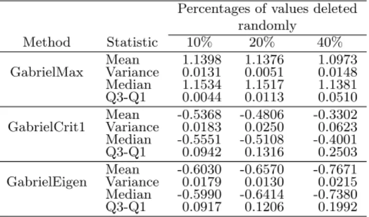
Table 1. Statistics of the standardized MSD.
Percentages of values deleted randomly
Method Statistic 10% 20% 40%
Mean 1.1398 1.1376 1.0973 GabrielMax Variance 0.0131 0.0051 0.0148 Median 1.1534 1.1517 1.1381 Q3-Q1 0.0044 0.0113 0.0510 Mean -0.5368 -0.4806 -0.3302 GabrielCrit1 Variance 0.0183 0.0250 0.0623 Median -0.5551 -0.5108 -0.4001 Q3-Q1 0.0942 0.1316 0.2503 Mean -0.6030 -0.6570 -0.7671 GabrielEigen Variance 0.0179 0.0130 0.0215 Median -0.5990 -0.6414 -0.7380 Q3-Q1 0.0917 0.1206 0.1992
missing values is GabrielMax.
The Friedman non-parametric test was used to investigate differences among the standardized MSD values for the three imputation methods in each percentage of missing values. The values of theTF riedman statistic
com-parisons among the imputation methods showed that there are significant differences of the MSD among the all methods. Similarly, applying the Levene test of variance homogeneity of the standardized MSD among the algorithms for the three percentages of missing values yielded values of the Levene statistic of 0.32 (p-value < 0.7245), 12.72 (p-value < 0.0001) and 54.18 (p-value < 0.0001) respectively, indicating rejection of the variance homogeneity hypothesis of the methods for the 20% and 40% percentages of missing values.
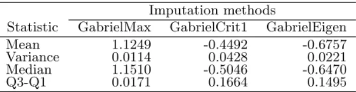
Table 2. General statistics of the standardized MSD.
Imputation methods
Statistic GabrielMax GabrielCrit1 GabrielEigen
Mean 1.1249 -0.4492 -0.6757
Variance 0.0114 0.0428 0.0221
Median 1.1510 -0.5046 -0.6470
Q3-Q1 0.0171 0.1664 0.1495
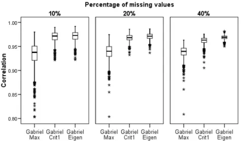
Finally, Table 2 shows the overall statistics obtained in the simulation study, irrespective of the percentages of missing values. The method that minimizes the interquartile distance is GabrielMax. GabrielEigen yields the lowest values of the MSD median and mean, while the minimal variance is achieved by GabrielMax. Overall the GabrielMax method gave the smallest variances, but this is only good if the mean/median are small too, and this was not the case here. So, according to the standardized MSD, the most efficient imputation method is GabrielEigen. Figure 2 presents the corre-lation coefficient distribution that was calculated in each simulated data set to compare the imputations with the real experimental data. It shows that the performance of the GabrielCrit1 and GabrielEigen algorithms is similar when imputing 10% and 20% of the data, with an approximately asymmetrical distribution and with correlations higher than 0.90. For 40% imputation, the method that presents the highest correlations and the mini-mal variability of the Pearson correlation coefficient in the simulation study is GabrielEigen. In all the percentages the GabrielMax method shows the greatest variability and the lowest values of the correlation coefficient. In general, according to the Pearson correlation coefficient the best method is GabrielEigen.
3.2. Example
Figure 2.Box plot of the correlation distribution between real and imputed data for 10%, 20% and 40% missing values.
of the standardized MSD and also obtaining the best correlations with the real data. So, to check the consistency of the results, another real data set was chosen from a trial with genotype-by-environment interaction, in order once again to apply the proposed imputation methods.
The data correspond to trials conducted in seven environments in the south and southeast regions of Brazil, for 20Eucalyptus grandis progenies from Australia. A randomized block design with 6 plants per plot and 10 replicates was used, the whole experiment taking up a space of dimension 3.0 m by 2.0 m. The original data and additional features of the trials can be found in Lavoranti (2003, p.91) and Bergamo (2007, p.33).
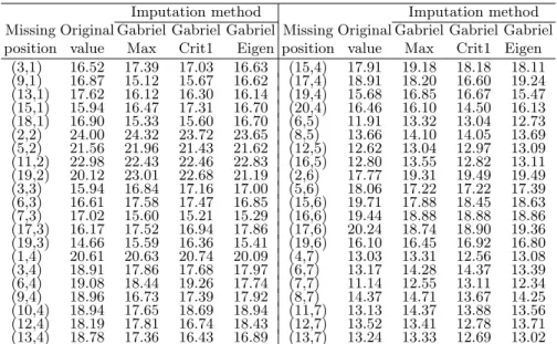
The data matrix has size 20×7, and unlike the simulation study, only a random withdrawal of 30% was considered and without repetitions, i.e. 42 missing values. The same situation was studied by Bergamo et al. (2008). The results obtained using GabrielMax, GabrielCrit1 and GabrielEigen are presented in Table 3.
Table 3. Estimates of missing values introduced into the data by random deletion.
Imputation method Imputation method
Missing Original Gabriel Gabriel Gabriel Missing Original Gabriel Gabriel Gabriel position value Max Crit1 Eigen position value Max Crit1 Eigen
(3,1) 16.52 17.39 17.03 16.63 (15,4) 17.91 19.18 18.18 18.11 (9,1) 16.87 15.12 15.67 16.62 (17,4) 18.91 18.20 16.60 19.24 (13,1) 17.62 16.12 16.30 16.14 (19,4) 15.68 16.85 16.67 15.47 (15,1) 15.94 16.47 17.31 16.70 (20,4) 16.46 16.10 14.50 16.13 (18,1) 16.90 15.33 15.60 16.70 (6,5) 11.91 13.32 13.04 12.73 (2,2) 24.00 24.32 23.72 23.65 (8,5) 13.66 14.10 14.05 13.69 (5,2) 21.56 21.96 21.43 21.62 (12,5) 12.62 13.04 12.97 13.09 (11,2) 22.98 22.43 22.46 22.83 (16,5) 12.80 13.55 12.82 13.11 (19,2) 20.12 23.01 22.68 21.19 (2,6) 17.77 19.31 19.49 19.49 (3,3) 15.94 16.84 17.16 17.00 (5,6) 18.06 17.22 17.22 17.39 (6,3) 16.61 17.58 17.47 16.85 (15,6) 19.71 17.88 18.45 18.63 (7,3) 17.02 15.60 15.21 15.29 (16,6) 19.44 18.88 18.88 18.86 (17,3) 16.17 17.52 16.94 17.86 (17,6) 20.24 18.74 18.90 19.36 (19,3) 14.66 15.59 16.36 15.41 (19,6) 16.10 16.45 16.92 16.80 (1,4) 20.61 20.63 20.74 20.09 (4,7) 13.03 13.31 12.56 13.08 (3,4) 18.91 17.86 17.68 17.97 (6,7) 13.17 14.28 14.37 13.39 (6,4) 19.08 18.44 19.26 17.74 (7,7) 11.14 12.55 13.11 12.34 (9,4) 18.96 16.73 17.39 17.92 (8,7) 14.37 14.71 13.67 14.25 (10,4) 18.94 17.65 18.69 18.94 (11,7) 13.13 14.37 13.88 13.56 (12,4) 18.19 17.81 16.74 18.43 (12,7) 13.52 13.41 12.78 13.71 (13,4) 18.78 17.36 16.43 16.89 (13,7) 13.24 13.33 12.69 13.02
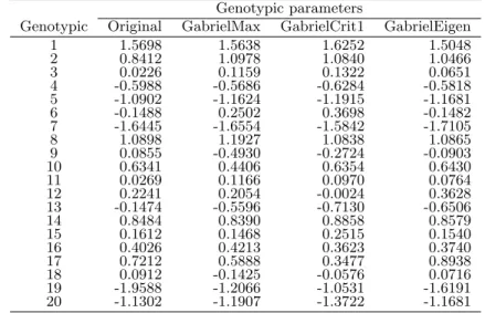
The results of the example and the simulation study, confirm that Gabriel-Eigen should be the recommended method. The GabrielCrit1 algorithm gave inconsistent results because its standardized MSD was smaller than GabrielMax in the simulation study, but in the example it had largest MSD. Since missing data are also predicted in order to complete tables of in-formation with the final goal of estimating model parameters, we fitted the genotypic and environmental parameters (i.e., the principal effects) using the analysis of variance ANOVA after the data imputation. The genotypic and environmental parameters of the original data and completed data are shown in Table 4 and Table 5. The genotype 1 and 19 have the most in-fluence in theE. grandis heights, positive and negative respectively; while the environments are highlighted on 2 and 5.
The MSDs among the genotypic parameters of the original data and the completed data were as follows: 0.0722 imputing with GabrielMax, 0.0957 using GabrielCrit1 and 0.0256 with the imputation through GabrielEigen. GabrielEigen again gives the best results.
Table 4. Fitted genotypic parameters by ANOVA in completed data.
Genotypic parameters
Genotypic Original GabrielMax GabrielCrit1 GabrielEigen
1 1.5698 1.5638 1.6252 1.5048
2 0.8412 1.0978 1.0840 1.0466
3 0.0226 0.1159 0.1322 0.0651
4 -0.5988 -0.5686 -0.6284 -0.5818
5 -1.0902 -1.1624 -1.1915 -1.1681
6 -0.1488 0.2502 0.3698 -0.1482
7 -1.6445 -1.6554 -1.5842 -1.7105
8 1.0898 1.1927 1.0838 1.0865
9 0.0855 -0.4930 -0.2724 -0.0903
10 0.6341 0.4406 0.6354 0.6430
11 0.0269 0.1166 0.0970 0.0764
12 0.2241 0.2054 -0.0024 0.3628
13 -0.1474 -0.5596 -0.7130 -0.6506
14 0.8484 0.8390 0.8858 0.8579
15 0.1612 0.1468 0.2515 0.1540
16 0.4026 0.4213 0.3623 0.3740
17 0.7212 0.5888 0.3477 0.8938
18 0.0912 -0.1425 -0.0576 0.0716
19 -1.9588 -1.2066 -1.0531 -1.6191
20 -1.1302 -1.1907 -1.3722 -1.1681
Table 5. Fitted environmental parameters by ANOVA in completed data.
Environmental parameters
Environment Original GabrielMax GabrielCrit1 GabrielEigen
1 -0.3468 -0.5274 -0.4067 -0.3904
2 5.6582 5.8021 5.7769 5.6990
3 -0.1378 -0.0109 0.0368 -0.0276
4 1.1922 0.9024 0.7520 0.9265
5 -4.2698 -4.1279 -4.1378 -4.1785
6 1.5312 1.3796 1.4955 1.5013
7 -3.6273 -3.4179 -3.5167 -3.5302
4. Conclusions
References
Arciniegas S. (2008): Imputa¸c˜ao de dados em experimentos com intera¸c˜ao genótipo por ambiente: uma aplica¸c˜ao a dados de algod˜ao. MSc thesis (in Portuguese) - Universidade de S˜ao Paulo (accessed in March 23, 2009). http://www.teses.usp.br/teses/disponiveis/11/11134/tde-11032009-150202/ Arciniegas-Alarcón S., Dias C.T.S. (2009): Imputa¸c˜ao de dados em experimentos
com intera¸c˜ao genótipo por ambiente: uma aplica¸c˜ao a dados de algod˜ao. Revista Brasileira de Biometria 27 (1): 125–138.
Bello A.L. (1993): Choosing among imputation techniques for incomplete multi-variate data: a simulation study. Communications in Statistics - Theory and Methods 22 (3): 853–877.
Bergamo G.C. (2007): Imputa¸c˜ao m´ultipla livre de distribui¸c˜ao utilizando a decomposi¸c˜ao por valor singular em matriz de intera¸c˜ao. PhD thesis (in Portuguese), Universidade de S˜ao Paulo (accessed in March 23, 2009). http://www.lce.esalq.usp.br/tadeu/genevile bergamo tese.pdf
Bergamo G.C., Dias C.T.S., Krzanowski W.J. (2008): Distribution-free multiple imputation in an interaction matrix through singular value decomposition. Scientia Agricola 65 (4): 422–427.
Caliński T., Czajka S., Denis J.B., Kaczmarek Z. (1992): EM and ALS algorithms applied to estimation of missing data in series of variety trials. Biuletyn Oceny Odmian 24-25: 7–31.
Caliński T., Czajka S., Denis J.B., Kaczmarek Z. (1999): Further study on esti-mating missing values in series of variety trials. Biuletyn Oceny Odmian 30: 7–38.
Denis J.B. (1991): Ajustements de mod`eles lin´eaires et bilin´eaires sous contraintes lin´eaires avec donn´ees manquantes. Revue de statistique appliqu´ee 39 (2): 5–24.
Denis J.B., Baril C.P (1992): Sophisticated models with numerous missing values: the multiplicative interaction model as an example. Biuletyn Oceny Odmian 24-25: 33–45.
Dias C.T.S., Krzanowski W.J. (2003): Model selection and cross validation in additive main effect and multiplicative interaction models. Crop Science 43: 865–873.
Dias C.T.S., Krzanowski W.J. (2006): Choosing components in the additive main effect and multiplicative interaction (AMMI) models. Scientia Agricola 63 (2): 169–175.
Dodge Y. (1985): Analysis of experiments with missing data. John Wiley, New York.
Farias F.J.C. (2005): ´Indice de sele¸c˜ao em cultivares de algodoeiro herb´aceo. PhD thesis (in Portuguese) - Universidade de S˜ao Paulo (accessed in March 23, 2009). http://www.teses.usp.br/teses/disponiveis/11/11137/tde-12012006-162727/publico/FranciscoFarias.pdf
Freeman H. G. (1975): Analysis of interactions in incomplete two-ways tables. Applied Statistics 24 (1): 46–55.
Gabriel K. R. (2002): Le biplot - outil d´exploration de donn´ees multidimen-sionelles. Journal de la Societe Francaise de Statistique 143: 5–55.
Gauch H.G. (1988): Model selection and validation for yield trials with interaction. Biometrics 44 (3): 705–715.
Gauch H.G. (1992): Statistical Analysis of Regional Yield Trials: AMMI Analysis of Factorial Designs. Elsevier, Amsterdam.
Gauch H.G., Zobel R.W. (1990): Imputing missing yield trial data. Theoretical and Applied Genetics 79: 753–761.
Godfrey A.J.R., Wood G.R., Ganesalingam S., Nichols M.A., Qiao C.G. (2002): Two-stage clustering in genotype-by-environment analyses with missing data. Journal of Agricultural Science 139: 67–77.
Good I.J. (1969): Applications of the singular decomposition of a matrix. Techno-metrics 11 (4): 823–831.
Krzanowski W.J. (1988): Missing value imputation in multivariate data using the singular value decomposition of a matrix. Biometrical Letters XXV (1,2): 31–39.
Lavoranti O.J. (2003): Estabilidade e adaptabilidade fenot´ıpica atrav´es de reamostragem “bootstrap” no modelo AMMI. PhD thesis (in Por-tuguese) - Universidade de S˜ao Paulo (accessed in March 23, 2009). http://www.teses.usp.br/teses/disponiveis/11/11134/tde-22102003-160700/ Little R. J., Rubin D.B. (2002): Statistical analysis with missing data. John Wiley,
New York.
Mandel J. (1993): The analysis of two-way tables with missing values. Applied Statistics 42 (1): 85–93.
Piepho H.P. (1995): Methods for estimating missing genotype-location combina-tions in multilocation trials - an empirical comparison. Informatik, Biometrie und Epidemiologie in Medizin und Biologie 26 (4): 335–349.
SAS INSTITUTE. (2004): SAS/IML 9.1 User.s guide. Carey: SAS Institute Inc. Sprent P., Smeeton N.C. (2001): Applied Nonparametric Statistical Methods.
Chapman and Hall, London.