Diffraction and reflection of irregular waves in a harbor employing a spectral model

(1)

(Annals of the Brazilian Academy of Sciences) ISSN 0001-3765

www.scielo.br/aabc

Diffraction and reflection of irregular waves in a harbor

employing a spectral model

NELSON VIOLANTE-CARVALHO1, RAFAEL B. PAES-LEME1, DOMENICO A. ACCETTA2 and FREDERICO OSTRITZ1 1_{Faculdade de Oceanografia, Universidade do Estado do Rio de Janeiro/UERJ}

Rua São Francisco Xavier, 524, 4015E, 20550-900 Rio de Janeiro, RJ, Brasil

2_{Instituto Nacional de Pesquisas Hidroviárias/INPH}

Rua General Gurjão, 166, 20930-040 Rio de Janeiro, RJ, Brasil

Manuscript received on June 11, 2008; accepted for publication on June 17, 2009; presented byALCIDESN. SIAL

ABSTRACT

The SWAN wave model is widely used in coastal waters and the main focus of this work is on its application in a harbor. Its last released version – SWAN 40.51 – includes an approximation to compute diffraction, however, so far there are few published works that discuss this matter. The performance of the model is therefore investigated in a harbor where reflection and diffraction play a relevant role. To assess its estimates, a phase-resolving Boussinesq wave model is employed as well, together with measurements carried out at a small-scale model of the area behind the breakwater. For irregular, short-crested waves with broad directional spreading, the importance of diffraction is relatively small. On the other hand, reflection of the incident waves is significant, increasing the energy inside the harbor. Nevertheless, the SWAN model does not achieve convergence when it is set to compute diffraction and reflection simultaneously. It is concluded that, for situations typically encountered in harbors, with irregular waves near reflective obstacles, the model should be set without the diffraction option.

Key words:wind waves, SWAN model, wave reflection, wave diffraction, wave transformations in a harbor.

INTRODUCTION

Wave exposure is an important consideration in plan-ning, designing and operating in the coastal zone. Care-ful analysis is necessary to determine the main charac-teristics of the waves as significant height, period and direction of propagation covering intervals of time long enough for the characterization of their spatial and tem-poral variability. In order to do so, wave measurements are employed, with sensors operating remotely such as altimeters (Robinson 2004, Chelton et al. 2001) and Syn-thetic Aperture Radars (Violante-Carvalho et al. 2005, Rousseau and Forget 2001), or in situ as buoys and PUV gauges (Tucker and Pitt 2001).

Correspondence to: Nelson Violante-Carvalho

E-mail: [email protected]; [email protected]

The description of the variability of the wave cli-mate is of utmost importance for the construction of any coastal structure such as groins, seawalls, jetties and breakwaters. A considerable part of the energy trans-ferred from the atmosphere to the ocean is carried on in the form of wind waves, which is released very quickly in the surf zone affecting the local hydrodynamics, the transport of sediments and the coastal morphology. Ex-posure analysis is used to evaluate the need to reduce wave energy, while the investigation of wave energy dis-sipation is required to support the design of these coastal structures.

(2)

wave agitation should be explored in either a mathe-matical or physical model in order to arrive at an opti-mum harbor layout. Wind waves are the main respon-sible for the movement of moored vessels from their berthing positions, causing efforts in mooring cables and structures of the pier. The propagation of waves in the vicinity of breakwaters is a complex process that involves shoaling, refraction, diffraction and reflection (Losada et al. 1990, Dingemans 1997, Cho et al. 2001, Ocampo-Torres 2001).

With the advance of computer science, numerical models have been widely improved. However, to be used effectively, it is important that the data are sup-plied to the model with wealth of details. Modeling an area around a breakwater is a difficult task for numer-ical models due to the complex transformations under-gone by the water waves. From the point of view of coastal research, an effective option would be to employ a numerical model and a small scale physical model, simultaneously, together with wave measurements car-ried out in the area.

Numerical models may be employed to estimate the main wave characteristics. They can be divided into two general classes (Young 1999): phase resolving and phase averaging models. Phase resolving models pre-dict both the amplitude and phase of the waves, but are computationally much more demanding. Among the main physical processes of interest, only diffraction and three wave interactions require phase resolving models, hence its applications are generally confined to small areas around harbors and the nearshore zone. Phase av-eraging models, on the other hand, predict average quan-tities such as the spectrum or significant wave height. If the wave properties vary slowly over a length of order 10 wavelengths or more, computations over large areas are feasible and phase averaging models are more con-venient than phase resolving models.

The most employed phase resolving models are those based either on the Mild Slope Equation derived by Berkhoff (1972) or on the Boussinesq Equations (Madsen et al. 1991, Madsen and Sorensen 1992). These models have been applied mainly to the areas where there is an interaction between the waves and any structure like a breakwater or an island. They do not, or only to some extent, account for wave-wave

inter-actions, generation and dissipation and require a high spatial resolution over the entire computational region.

Spectral (phase averaging) models, such as WAM (WAMDI Group 1988), WAVEWATCH III (Tolman 1991) and SWAN (Booij et al. 1999), can account for the processes of generation, propagation, refraction, dissipation and wave-wave interactions. However, these models are not normally used to account for diffrac-tion. In coastal regions, diffraction plays a relevant role in the wave transformations, especially around emerged structures. In general so far, phase-averaged models have been used to estimate the wave conditions in the coastal area and phase-resolving models have been used to compute the wave conditions in the nearshore zone. Recently, a phase-decoupled refraction-diffraction ap-proximation has been incorporated into the spectral wave model SWAN (Holthuijsen et al. 2003), widen-ing its range of applications. Phase-averaged are more efficient than phase-resolving models, therefore, the in-corporation of a diffraction approximation into spectral models is a highly desirable feature.

For any coastal study, another possible approach is the construction of physical models of a particular region, as a harbor, represented in scale in the labora-tory. Small scale physical models are very useful for developing, improving or testing numerical models, which mainly rely on empirical parameters and on field measurements affected by large uncertainties. They al-low the representation of structures, in reduced scale, for understanding their behavior when subjected to en-vironmental conditions. Its main purpose is the repres-entation of possible situations that are not easily tract-able analytically.

(3)

the understanding of the effect of diffraction estimated by the SWAN in a harbor, its performance is compared with a small scale model and the numerical model MIKE BW 21 (DHI 1998), a phase-resolving model based on the Boussinesq equations. The structure of the paper is as follows. First, the study area is described in Section 2, while the SWAN and the MIKE BW 21 models are discussed in Section 3. The methodology employed is described in Section 4 and the results are given in Section 5. Section 6 concludes with a summary and main recommendations.

STUDY AREA

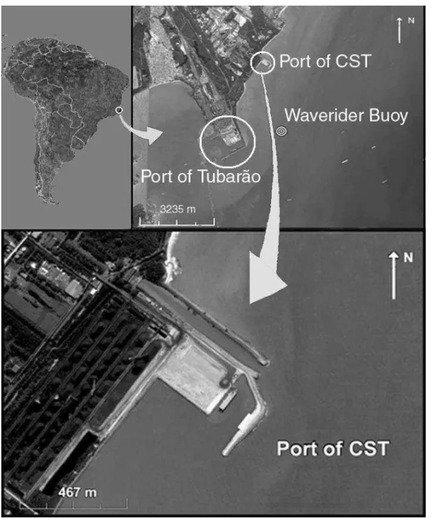
The study area (Fig. 1), the port of the Tubarão Siderur-gic Company (CST, from its acronym in Portuguese), lies between latitudes 20◦₁₄′_{S and 20}◦₁₉′_{S and} longi-tudes 40◦12′W and 40◦15′W. The worldwide leader in producing steel slabs, CST is located in the city of Vitória, Espírito Santo State, Southeastern Brazil. Vitó-ria, in general, is subject to waves of higher energy from the southern quadrant, associated with the pas-sage of frontal systems (INPH 2003a).

A directional Waverider was deployed during 198 days, from May 28, 2001 until December 11, 2001, by the Brazilian Waterways Research Institute (INPH) off the Port of Tubarão (located in the vicinity of CST, Fig. 1). The buoy measures vertical and horizontal accelerations using accelerometers and an onboard com-pass to give the directional displacement in two hori-zontal axes. The instrument was moored in 20◦17′18′′S and 40◦12′54′′W, in a water depth of approximately 21 m. Conventional Fourier techniques were employed for the buoy data analysis, as described in Violante-Car-valho and Robinson (2004).

Measurements did not cover a full year, which is the minimum time required for the characterization of the seasonal variability in a region. However, they were carried out during the period considered most critical for the operation of the harbor. During the Southern Hemisphere winter and spring, extra-tropical cyclones pass over the area more often with the consequent in-crease in wave energy (INPH 2003b). The higher en-ergy events were selected from the data gathered by the Waverider and employed for simulations with the numerical models. The most unfavorable conditions

of operation inside the harbor were determined, which were employed for the configuration of the physical model.

NUMERICAL MODELS

SWAN

SWAN (Simulating WAves Nearshore) is a third gen-eration numerical model developed for wave computa-tions in coastal regions (see the ‘SWAN book’ Holthuij-sen 2007, chapter 9). The model uses the action bal-ance to compute the evolution of the wave field in time and space, given by:

∂ ∂tN +

∂

∂xcxN +

∂ ∂ycyN

+ ∂

∂σcσN + ∂

∂θcθN = ∂S

∂σ.

(1)

The action balance equation (1) is a first-order partial differential equation with five independent vari-ables: time (t), the two horizontal coordinates (x,y), relative frequency(σ )and direction of propagation(θ ). The first term on the left hand side of (1) represents the rate of change of action (or energy) density in time, where N(σ, θ )is the action density spectrum. The sec-ond and third terms indicate propagation of action in the geographical area (with speeds of propagation cx

andcy inx andy, respectively). The fourth term deals

with changes of the relative frequency due to variations in depth and currents (with velocity of propagationcσ). The fifth term represents refraction induced by varia-tions in depth and currents (with velocity of propaga-tioncθ). The source term S (= S(σ, θ )) represents the effects of generation, dissipation and non-linear wave-wave interactions.

(4)

Fig. 1 – The study area, off of the city of Vitória, Espírito Santo State, Southeastern Brazil. The Waverider buoy position is also shown, together with the Port of CST and the Port of Tubarão. Source: Google Earth.

The steady state solution, hence neglecting the first term on the left hand side of (1), is achieved through a number of iterations. The propagation step in the geographical space is carried out for each grid point decomposing the directional space in four quad-rants. In each quadrant the computations are carried out independently of the other quadrants with propagation of these components called sweep. By rotating each quadrant of 90◦ becomes possible to propagate energy in all directions over the entire geographical domain.

However, effects that can change the direction of propagation of the wave components, as refraction

(5)

previously stipulated, is achieved whether the process turned out to converge or not.

The effects of refraction are easily accounted for with phase-averaged models. Diffraction, on the other hand, is incorporated into the model as presented in Hol-thuijsen et al. (2003). The approximation is based on the Mild Slope Equation for refraction-diffraction, omitting, however, information about the phase of the waves. The implementation is achieved by adding a parameterδE to the propagation velocitiescx, cy and cθ given by

δE =

∇ •ccg∇√E

κ2_cc

g √

E , (2)

wherecandcgare the phase and group velocity,

respec-tively. The energy density is represented byE₌E(σ, θ ) andκis a separation parameter.

Apart form the possibility of turning diffraction on and off, the model has some programmable parameters to control how diffraction is computed. The parameters SMPAR and SMNUM are basically used to control the amount of smoothing among adjacent grid points, avoid-ing numerical instabilities (SWAN Team 2006).

MIKE 21 BW

The phase-resolving model MIKE 21 BW is based on the numerical solution of a new formulation of the Boussinesq equations, derived by Madsen et al. (1991) and Madsen and Sorensen (1992). The main limitation of the classical Boussinesq equations lies on the cal-culation of wave propagation in deep water. However, its enhanced formulation with improved frequency dis-persion makes the model appropriate for simulation of wave propagation from deep water through shallow water. A major engineering application of the model is the assessment of disturbance inside harbors aiming to determine its optimum layout.

The model is capable of reproducing the combined effects of most physical processes of interest in shal-low water, such as shoaling, refraction, diffraction and reflection of directional, irregular waves of finite am-plitude propagating over complex bathymetries (DHI 1998). It can be applied for the determination of the wave-induced hydrodynamics in coastal areas, as well as for the analysis of oscillations caused by regular and

irregular waves in enclosed basins (Hansen et al. 2005). The version employed here does not include realistic approaches for the mechanism of wave breaking. Con-sequently, the model should not be extended into the surf zone where wave breaking is important, which is not the case in the present investigation. Hansen et al. (2005) and Sorensen et al. (2004) report the results of some models based on the Boussinesq equations that include wave breaking in their calculations.

The main aim of the present study is to evaluate the efficiency of the SWAN model in situations where diffraction is important; therefore, the description of the model MIKE 21 BW is kept to a minimum. Further details of its main features are described in the opera-tion manual (DHI 1998).

MATERIALS AND METHODS

A bathymetric survey was conducted in the Espírito Santo Bay by INPH in 1999 and in 2002 by Argos Hydrographic Services Limited. In the region further away from the coast the bottom topography was deter-mined from the nautical chart DHN 1410, published by the Brazilian Navy Hydrographic Center.

Simulations performed with MIKE 21 BW indi-cated that the most unfavorable conditions of operation inside the harbor occur when the direction of wave propagation offshore is from 150◦_{(INPH 2003b). This} was, therefore, the direction chosen to set up the phys-ical model. Among the data gathered by the Waverider buoy, 4 records were selected with mean wave direc-tion around 150◦and significant height of 1.0 m, 1.5 m, 2.0 m and 2.5 m. The main parameters of selected records of the buoy data used as boundary conditions for the physical model and for the numerical models are listed in Table I.

SCALEMODELEXPERIMENTATION

(6)

TABLE I

Measurements made by the Waverider buoy used as

boundary conditions for the physical model and for the

numerical models. The values listed are Peak Period

(Peak Per), Mean Period (Mean Per), Significant Wave

Height (Sig Hei) and Mean Direction (Mean Dir), the

direction waves are coming from (compass bearing).

Record Peak Per Mean Per Sig Hei Mean Dir

1 9.1 s 6.1 s 0.99 m 145.5◦

2 7.7 s 5.9 s 1.49 m 149.7◦

3 8.3 s 5.8 s 2.00 m 154.6◦

4 10.5 s 6.4 s 2.51 m 144.2◦

A wave gage array of 8 sampling elements was de-signed to provide estimates of significant wave height within the physical model. The wave gage operates with a submerged, insulated wire rod. The time-varying height of the water surface creates a varying capacitance that is transmitted to a converter yielding an output volt-age proportional to the wave height, later scaled up to natural scale (INPH 2003b).

The position of the 8 wave rods relative to the harbor lay out is presented in Figure 2. The measured field data from the physical model and the calculated data from the two wave models can then be compared. Statistical comparisons were performed with the wave rods displaced over two lines. Line 1 consists of the wave rods numbered as 11, 5, 10, 4 and 9. The outer wave rod number 11, in the less sheltered position, is spaced by a distance from the others of, respectively, 50, 90, 130 and 170 m in the real world scale. Line 2 is composed by rods number 6, 7 and 8. The outer one, number 6, is spaced from the other two of 30 and 190 m, respectively.

NUMERICALIMPLEMENTATION

Simulations with the models were performed and the measured directional spectra were taken as input at all boundary grid points. Both models were run in sta-tionary mode on a regular grid in Cartesian coordinates. Comparisons of the measured data from the physical model and the calculated data from SWAN and MIKE 21 BW were performed for the computational grid points that correspond to the wave rods. The

re-flection coefficient chosen (0.40) for both models is typical for rubble mound breakwaters (DHI 1998). Ef-fects such as wind input, whitecapping, currents and wave-wave interactions (triad or quadruplet) were not included in the present study.

MIKE 21 BW was run with a grid spacing of 8 m with a total of 651 by 1021 points. Sponge and porosity layers were used to model absorption and re-flection areas through the computational domain. The area around the Port of CST was set as a porosity layer to model partial reflections around the breakwater, while the remaining area was set as a sponge layer absorbing all incoming wave energy.

SWAN simulations, on the other hand, were com-puted on a coarser grid of 131 by 205 points (grid spac-ing of 40 m) to reduce computational time. In the area closer to the port, shown in Figure 2, model estimations were achieved by nesting a finer grid run, with resolu-tion of 8 m, in the coarse grid run. Ilica et al. (2007) present several simulations employing SWAN (with dif-fraction) to determine the optimum grid size with the lowest error and fewer cycles to achieve a stable solu-tion. In that work, the best results were achieved when the ratio between the wavelength corresponding to the peak period and grid size Lp

1x

was from 10 to 15. For larger grid sizes, fewer cycles were necessary to obtain a stable solution. However, increasing grid size worsens the results around tip of structures such as breakwaters (Enet et al. 2006) and a compromise between grid size and model performance must be sought. In the present work, with a grid resolution of 8 m, the ratio₁Lp_x is 16.3, 11.5, 13.4 and 21.4, respectively, for the different simu-lations shown in Table I.

Wave reflection in SWAN is computed setting the coordinates of obstacle lines and a constant reflection coefficient. The position of the obstacle lines in the sur-roundings of the Port of CST is also depicted in Fig-ure 2. Additionally, several combinations of the diffrac-tion smoothing parameters SMNUM and SMPAR were tested without significant changes in the results, hence their default values were used.

DESCRIPTION AND RESULTS OF THE SIMULATIONS

(7)

Fig. 2 – Obstacle lines represented by the dark gray lines around the Port of CST, where reflection is computed by the SWAN model. The position of the wave rods in the computational domain is also shown, which are the grid points where significant wave height were estimated by the numerical models. The figure represents the region between latitudes 20◦15′35′′S and 20◦15′47′′S and longitudes 40◦13′21′′W and 40◦13′01′′W.

in the harbor and test their results against measurements obtained by the wave rods in the physical model. In order to assure that, different configurations were im-plemented with the SWAN model. At first, simulations were conducted with diffraction and without reflection (the obstacle lines were not habilitated). In all tests, the model yielded stable solutions after around 10 cycles. A second test was performed without diffraction and with reflection, with stable solutions obtained after around five cycles.

A third configuration, using diffraction and reflec-tion simultaneously, was performed, but the simulareflec-tions did not converge. After the few initial iterations (from six to nine) the accuracy drops from over 90% of the wet grid points to less than 10% and remains low. How-ever, for each of the four simulations with different inci-dent significant wave heights, the values over the wave rod lines for the iteration obtaining the highest accu-racy were compared to the values of the subsequent iterations. The maximum differences, in most of the cases, were less than 1 cm. Therefore, the values of the iteration with the maximum accuracy were used for fur-ther comparisons even if the model did not turn out to

converge. The three configurations (with and without diffraction and reflection) were then employed to in-vestigate the importance of diffraction and reflection in SWAN simulations in a harbor.

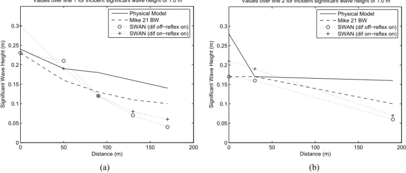
Figures 3, 4, 5 and 6 show the results for the phys-ical model, for MIKE 21 BW run and for two differ-ent runs of the SWAN model (with reflection and with/ without diffraction). The figures correspond, respec-tively, to incident wave heights of 1.0, 1.5, 2.0 and 2.5 m and the two lines where the wave rods were dis-placed (Fig. 2). It is clear from the figures that higher incident waves correspond to higher energy in the port. The significant wave height measured in the physical model decreases from the outer region (represented by the value 0 on the horizontal axis) towards the sheltered region. Similar results were given by MIKE 21 BW in most of the simulations except in Figure 4b (where sig-nificant wave height in rod number 7 is 1 cm higher than in number 6) and in Figure 6b, where significant wave height in rod number 6 is much higher than in number 7 and the curve exhibits an abrupt slope. The same pat-tern of energy decay towards the inner part of the port is observed with the SWAN estimates but for Figure 6b, where significant wave height in rod number 7 is higher than in number 6.

The plots corresponding to the wave rods over line 1 – Figures 3a, 4a, 5a and 6a – show that the mod-els results are similar, independent of the incident wave height. In general, MIKE 21 BW underestimates the re-sults from the physical model, however comparatively, its values are closer to measurements than SWAN runs. The pattern of the SWAN runs is somehow more er-ratic, in general underestimating the data derived from the physical model in the sheltered part of the port and overestimating in the outer part. It is also worth mention-ing that SWAN predictions with diffraction are higher than without diffraction. In the outer wave rod (num-ber 11), SWAN estimates without diffraction are slightly better than with diffraction.

(8)

0 50 100 150 200 0 0.05 0.1 0.15 0.2 0.25 0.3 Distance (m) S ig n if ica n t W a ve H e ig h t (m)

Values over line 1 for incident significant wave height of 1.0 m

Physical Model Mike 21 BW SWAN (dif off−reflex on) SWAN (dif on−reflex on)

0 50 100 150 200

0 0.05 0.1 0.15 0.2 0.25 0.3 Distance (m) S ig n if ica n t W a ve H e ig h t (m)

(a) (b)

Fig. 3 – Significant wave height measured in the physical model and estimated by the models MIKE 21 BW and SWAN with reflection on for: diffraction off (dif off—reflex on) and diffraction on (dif on—reflex on). For incident significant wave height of 1.0 m (over Line 1 (a) and over Line 2 (b)).

0 50 100 150 200

0 0.05 0.1 0.15 0.2 0.25 0.3 0.35 0.4 0.45 Distance (m) S ig n if ica n t W a ve H e ig h t (m)

0 50 100 150 200

0 0.05 0.1 0.15 0.2 0.25 0.3 0.35 0.4 0.45 Distance (m) S ig n if ica n t W a ve H e ig h t (m)

(a) (b)

an incident significant wave height of 2.5 m (Fig. 6b). As over line 1, SWAN estimates with diffraction are higher than without diffraction and are closer to the physical model predictions. However, in the more shel-tered positions (wave rods number 4 and 9 over line 1 and 1 and 8 over line 2) the difference among SWAN predictions with and without diffraction is small, never more than 6 cm.

(9)

0 50 100 150 200 0 0.1 0.2 0.3 0.4 0.5 0.6 Distance (m) S ig n if ica n t W a ve H e ig h t (m)

Physical Model Mike 21 BW

SWAN (dif off−reflex on) SWAN (dif on−reflex on)

0 50 100 150 200

0 0.1 0.2 0.3 0.4 0.5 0.6 Distance (m) S ig n if ica n t W a ve H e ig h t (m)

SWAN (dif off−reflex on) SWAN (dif on−reflex on)

(a) (b)

0 50 100 150 200

0 0.1 0.2 0.3 0.4 0.5 0.6 0.7 0.8 Distance (m) S ig n if ica n t W a ve H e ig h t (m)

0 50 100 150 200

0 0.1 0.2 0.3 0.4 0.5 0.6 0.7 0.8 Distance (m) S ig n if ica n t W a ve H e ig h t (m)

(a) (b)

with SWAN runs is slightly lower,r=0.86 and 0.80 and s =13 and 12 cm, respectively, for configuration with and without diffraction. As a matter of comparison, the correlation coefficient between SWAN with and without diffraction is 0.96 with standard deviation of 13 cm.

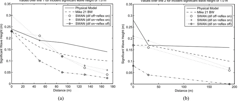
Additional tests, shown in Figure 7, were conducted without reflection and with diffraction for incident

(10)

0 20 40 60 80 100 120 140 160 180 0

0.05 0.1 0.15 0.2 0.25 0.3 0.35

Distance (m)

S

ig

n

if

ica

n

t

W

a

ve

H

e

ig

h

t

(m)

SWAN (dif off−reflex on) SWAN (dif on−reflex on) SWAN (dif on−reflex off)

0 50 100 150 200

0 0.05 0.1 0.15 0.2 0.25 0.3 0.35

Distance (m)

S

ig

n

if

ica

n

t

W

a

ve

H

e

ig

h

t

(m)

SWAN (dif off−reflex on) SWAN (dif on−reflex on) SWAN (dif on−reflex off)

(a) (b)

Fig. 7 – Significant wave height measured in the physical model and estimated by the models MIKE 21 BW and SWAN with reflection on for: diffraction off (dif off—reflex on) and diffraction on (dif on—reflex on). The values for reflection off and diffraction on (dif on—reflex off) are also shown. For incident significant wave height of 1.0 m; over Line 1 (a) and over Line 2 (b).

Due to the lack of convergence when SWAN was run with diffraction and with reflection, the choice seems to be either with diffraction and without reflection or without diffraction and with reflection. The results indi-cate that taking reflection into consideration has a greater relative importance for prediction of wave energy in the harbor. The mean differences between SWAN estim-ates without diffraction and with reflection and the physical model measurements are, respectively, of 6, 8, 9 and 13 cm for incident wave heights of 1.0, 1.5, 2.0 and 2.5 m. These values correspond to 6, 5.3, 4.5 and 5.2% of the incident significant wave height. Moreover, it is worth to stress that smaller differences were ob-tained when the model was tested with both diffraction and reflection, although it did not turn out to converge.

SUMMARY AND CONCLUSIONS

Analysis of wave interaction with breakwaters in gen-eral are performed using numerical models or small scale physical models. In the present study, both approaches were employed to assess practical limitations regarding the applicability of the combined effect of diffraction and reflection in the SWAN model computing waves in a harbor. In addition, the results of a phase-resolving model were also available, together with measurements made by a Waverider buoy. The validation tests revealed

that SWAN did not converge when set up with reflection and diffraction simultaneously, becoming unstable, re-vealing limitations to the use of diffraction in the model. Previous studies have questioned the need to com-pute wave diffraction in the lee of a breakwater for broad directional spread (as in, for example, Briggs et al. 1995). There is a direct relation between directional spread and wave diffraction. For short crested, irregular waves, with broad directional spread, more energy will be diffracted into the lee of the breakwater than for an equivalent monochromatic, long crested wave. There-fore, several computations were made with and without diffraction. The simulations confirmed that for irregu-lar, short crested waves, the difference in the results with and without diffraction is small and the effect of direc-tional spreading reduces the importance of diffraction. However, the model with the diffraction option enabled predicts the wave heights slightly better than the model without diffraction – although it did not turn out to con-verge – meaning a gain in the model results with the new phase-decoupled refraction-diffraction approximation.

(11)

undesirable oscillations. In the SWAN runs with diffrac-tion and without reflecdiffrac-tion effects, the values computed were much smaller than the physical model data and, in some situations, the significant wave height in the most sheltered positions was zero. The results indicate that reflection has, comparatively, a greater importance.

With the configurations presented here in, SWAN achieves convergence only when it is not set up to com-pute diffraction and reflection simultaneously. The best or most probable explanation, according to Holthuijsen (2007), is that the diffraction option should not be used in front of reflecting obstacles, as in the present case. In such situations, stationary waves can occur and phase information is necessary, which is not available. There-fore, in conditions usually found in harbors with broad directional spread, short crested irregular waves, SWAN 40.51 should be implemented without diffraction and with reflection to assure that it will achieve convergence. Naturally, phase resolving models are more appropriate in such situations, however, the rms difference between SWAN estimates without diffraction and with reflection and the physical model data is 10 cm and the mean dif-ference is around 5% of the incident significant wave height. Since SWAN is currently under continuous de-velopment, it is expected that such limitations, i.e. the problem of convergence, will be eliminated in future versions of the model.

RESUMO

O modelo de ondas SWAN é amplamente empregado em

simu-lações na região costeira e o presente trabalho investiga sua

aplicação dentro de um porto. A última versão disponibilizada

para a comunidade – SWAN 40.51 – inclui uma aproximação

para computar a difração, embora, até o momento, poucos

tra-balhos abordando este tema foram publicados. O desempenho

do modelo é estudado em um porto onde os fenômenos de

reflexão e difração são importantes. Para avaliar suas

estima-tivas, um modelo do tipo Boussinesq também é empregado,

juntamente com medições realizadas em um modelo em escala

reduzida da área atrás do quebramar. Para ondas irregulares,

com cristas curtas e espalhamento direcional mais amplo, a

importância da difração é relativamente menor. Contudo, o

modelo SWAN não alcança convergência quando programado

para estimar difração e reflexão simultaneamente. Conclui-se

que, para situações normalmente encontradas em portos, com

ondas irregulares próximas a obstáculos refletivos, o modelo

deve ser empregado sem a opção de difração.

Palavras-chave: ondas geradas pelo vento, modelo de

gera-ção e propagagera-ção de ondas SWAN, reflexão de ondas, difragera-ção

de ondas, transformação de ondas em um porto.

REFERENCES

BERKHOFF JCW. 1972. Computation of combined refrac-tion-diffraction. In: Proceedings 13thInt. Conf. Coastal Eng., ASCE, Vancouver, p. 471–490.

BOOIJN, RISRANDHOLTHUIJSENL. 1999. A third gener-ation wave model for coastal regions – 1. Model descrip-tion and validadescrip-tion. J Geophys Res 104(C4): 7649–7666.

BRIGGS MJ, THOMPSON EF AND VINCENT CL. 1995.

Wave diffraction around breakwater. J Waterw Port Coast Ocean Eng 121: 23–35.

CHELTONDB, RIESJ, HAINESBJ, FULLANDCALLA -HANP. 2001. Satellite altimetry. In: FULLANDCAZA -NAVE A (Eds), Satellite altimetry and earth sciences. Academic Press, 463 p.

CHOYS, YOONS, LEEJIANDYOONTH. 2001. A con-cept of beach protection with submerged breakwaters. J Coastal Res 34: 671–678.

DHI. 1998. MIKE 21 – User guide and reference manual, release 2.7. Technical report, Danish Hydraulic Institute. Denmark, 98 p.

DINGEMANSMW. 1997. Water wave propagation over un-even bottoms: Part 1 – linear wave propagation. World Scientific, London.

ENET F, NAHON A, VAN VLEDDER GAND HURDLE D.

2006. Evaluation of diffraction behind a semi-infinite breakwater in the SWAN Wave Model. In Proceedings of Ninth International Symposium on Ocean Wave Mea-surement and Analysis – WAVES06.

HANSEN KH, KERPERDR, SORENSENOR ANDKIRKE -GAARD DJ. 2005. Simulation of long wave agitation in ports and harbours using a time-domain Boussinesq model. In Proceedings of Fifth International Symposium on Ocean Wave Measurement and Analysis – WAVES 2005. Madrid, Spain.

HOLTHUIJSENLH. 2007. Waves in Oceanic and Costal Wa-ters. Cambridge University Press, Great Britain, 387 p.

HOLTHUIJSEN LH, HERMAN A AND BOOIJ N. 2003.

(12)

ILICAS,VAN DERWESTHUYSENBA, ROELVINKCJAND CHADWICK A. 2007. Multidirectional wave transfor-mation around detached breakwaters. Coastal Eng 54: 775–789.

INPH. 2003a. The evolution of wave generation systems in INPH. Technical report, Brazilian Waterways Research Institute (INPH). In Portuguese, 53 p.

INPH. 2003b. Mathematical modeling of wave propaga-tion around and inside the Port of CST. Technical report, Brazilian Waterways Research Institute (INPH). In Por-tuguese, 27 p.

LOSADAMA, DALRYMPLERAANDVIDALC. 1990. Water waves in the vicinity of breakwaters. J Coastal Res 7: 119–137.

MADSEN PANDSORENSENO. 1992. A new form of the Boussinesq equations with improved linear dispersion characteristics. Part 2. A slowly-varying bathymetry. Coastal Eng 18: 183–204.

MADSEN P, MURRAY IANDSORENSENO. 1991. A new form of the Boussinesq equations with improved linear dispersion characteristics. Coastal Eng 15: 371–388.

OCAMPO-TORRES FJ. 2001. On the homogeneity of the wave field in coastal areas as determined from ERS-2 and RADARSAT Synthetic Aperture Radar images of the ocean surface. Sci Mar 65(S1): 215–228.

ROBINSON IS. 2004. Measuring the Oceans from Space. Springer-Praxis Books, Great Britain, 669 p.

ROUSSEAUSANDFORGET P. 2001. Ocean wave mapping from ERS SAR images in the presence of swell and wind waves. Sci Mar 68(1): 1–5.

SORENSENOR, SCHAFFERHAANDSORENSENLS. 2004. Boussinesq-type modelling using an unstructured finite element technique. Coastal Eng 50: 181–198.

SWAN TEAM. 2006. Swan User Manual version 40.51. Department of Civil Engineering and Geosciences, Delft University of Technology, Delft, The Netherlands, 111 p.

TOLMANH. 1991. A third-generation model for wind waves on slowly varying, unsteady and inhomogeneous depths and currents. J Phys Oceanogr 21: 782–797.

TUCKERMJANDPITT EG. 2001. Waves in Ocean Engi-neering. Elsevier Engineering Book Series, Great Britain, 521 p.

VIOLANTE-CARVALHONANDROBINSONIS. 2004. On the retrieval of two dimensional directional wave spectra from spaceborne Synthetic Aperture Radar (SAR) images. Sci Mar 68(3): 317–330.

VIOLANTE-CARVALHO N, ROBINSON IS AND SCHULZ -STELLENFLETHJ. 2005. Assessment of ERS Synthetic Aperture Radar wave spectra retrieved from the MPI scheme through intercomparisons of one year of direc-tional buoy measurements. J Geophys Res 110(C07019).

WAMDI GROUP. 1988. The WAM model. A third genera-tion ocean wave predicgenera-tion model. J Phys Oceanogr 18: 1775–1810.

YOUNGIR. 1999. Wind Generated Ocean Waves. Elsevier, 288 p.

ZIJLEMAMAND VAN DERWESTHUYSENAJ. 2005. On