Bias in the prediction of genetic gain due to mass and half-sib selection in
random mating populations
José Marcelo Soriano Viana, Vinícius Ribeiro Faria and Admilson da Costa e Silva
Departamento de Biologia Geral, Universidade Federal de Viçosa, Viçosa, MG, Brazil.
Abstract
The prediction of gains from selection allows the comparison of breeding methods and selection strategies, although these estimates may be biased. The objective of this study was to investigate the extent of such bias in predicting ge-netic gain. For this, we simulated 10 cycles of a hypothetical breeding program that involved seven traits, three popu-lation classes, three experimental conditions and two breeding methods (mass and half-sib selection). Each combination of trait, population, heritability, method and cycle was repeated 10 times. The predicted gains were bi-ased, even when the genetic parameters were estimated without error. Gain from selection in both genders is twice the gain from selection in a single gender only in the absence of dominance. The use of genotypic variance or broad sense heritability in the predictions represented an additional source of bias. Predictions based on additive variance and narrow sense heritability were equivalent, as were predictions based on genotypic variance and broad sense heritability. The predictions based on mass and family selection were suitable for comparing selection strategies, whereas those based on selection within progenies showed the largest bias and lower association with the realized gain.
Key words:predicted genetic gain, realized genetic gain, recurrent selection. Received: April 16, 2008; Accepted: February 5, 2009.
Introduction
More than two decades ago, Wricke and Weber (1986) stated that the formula for predicting gain from se-lection “is certainly one of the central points in plant breed-ing research”. However, it is unlikely that either of these authors would now defend this position. Various relevant methods, such as selection indices, diallel analysis, stability and adaptability analysis, Best Linear Unbiased Prediction (BLUP) and QTL analysis, were developed by quantitative geneticists prior and after the proposition of a general func-tion for gain predicfunc-tion by Eberhart (1970). The predicfunc-tion function developed by Eberhart (1970) based on work by Falconer (1960) has proven useful for assessing the effi-ciency of breeding methods and selection strategies. Al-though regularly used in breeding studies, this function, popularly known as ‘the breeder’s equation’, is not the only one available to quantitative geneticists (Loywycket al., 2005).
Gonçalves et al. (2007) assessed several selection processes in families of yellow passion fruit obtained by Design I. The best process was combined selection. The predicted gain from combined selection based on the num-ber of fruits per plant was 18.55%, whereas the best results
for index-based selection were 15.92% for Pesek and Baker and 15.85% for Mulamba and Mock. In a study with BR 5011 corn cultivar in which three mass selection cycles and 17 cycles of half-sib selection were used, Carvalho and Souza (2007) predicted an average gain in yield of 2.56% in the last 14 cycles. Roseet al.(2007) assessed the efficiency of half-sib selection in switchgrass (Panicum virgatumL.) in high and low yield environments. The predicted gains for dry matter were generally lower in the unfavorable envi-ronment. The predicted gain for family selection was supe-rior to that for mass selection. Baltuniset al.(2007) showed that in loblolly pine (Pinus taedaL.) the predicted direct gain from half-sib selection for rooting ability was 36% while the predicted indirect gain for height at two years was 5.4%. Selecting the best families for height resulted in di-rect and indidi-rect predicted gains of 8.1% and 14.8%, re-spectively. The predicted direct gain from full-sib selection for rooting ability was 43% while the predicted indirect gain for height at two years was 9%. Selecting the best fam-ilies for height yielded direct and indirect predicted gains of 10.1% and 8.6%, respectively. The selection of clones based on rooting ability resulted in a predicted direct gain of 96% associated with a decrease in height. Selecting the best clones for height resulted in direct and indirect pre-dicted gains of 27% and 43%, respectively. Thus, overall, the selection indices assessed resulted in gains for both traits.
www.sbg.org.br
Send correspondence to José Marcelo Soriano Viana. Departa-mento de Biologia Geral, Universidade Federal de Viçosa, 36570-000 Viçosa, MG, Brazil. E-mail: [email protected].
Despite its usefulness in helping to choose the best breeding method or selection process, the Eberhart predic-tion formula is widely known to provide a biased estimate (usually an overestimate) of changes in the population mean. Bordeset al.(2006) compared the efficiency of two methods of corn inbred lines development. For yield, the use of the dihaploid method resulted in a predicted gain of 2%/year, which was lower than the predicted gains of 2.4%/year and 2.9%/year for two cycles of S1families, re-spectively, in four years. The real gains were 1.65%/year and 1.75%, respectively, indicating overestimation of the predicted gains. A study with popcorn showed that al-though there was agreement between the predicted and true mean gains in expansion volume and yield, the predictions per cycle were generally overestimated (Viana, 2007). Sim-ilar results are reported by Hallauer and Miranda Filho (1988).
In view of the lack of information on the relative im-portance of possible sources of bias, the aim of this study was to investigate biases in the prediction of genetic gains from selection.
Material and Methods
Sources of bias in the prediction of genetic gains
Although generally applicable to genetic breeding, the Eberhart function is based on mass selection in a single gender. The genetic gain (DM) is calculated as M1 - M, whereM1is the genotypic mean of the bred population and Mis the genotypic mean of the population in which the se-lection was made. The gain is proportional to the difference between the phenotypic mean of the selected population (Ps) and the phenotypic mean of the base population (P),
re-ferred to as the selection differential (SD), i.e.,
DM=b.(Ps-P). Thus,M1=M+b.SD. Since the bred popu-lation consists of half-sib families whose common parents are the selected individuals, the parameter b should be the same as the regression of the mean phenotypic value of progeny as a function of the difference between the pheno-typic value of the selected individual and the phenopheno-typic mean of the base population (Po Ps P i
i =b0+b1( i - )+e ,
assuming identity of the models for each selected individ-ual). Based on this assumption,
E Po M Ps P M bSD
i
( )= 1 =b0+b1( - )= + . In addition, as-suming that genotypic value and environmental effect are independent,
b P P
V P
G G
V P
s o s
s o s
=Cov( , )=Cov
( )
( , ) ( )
whereGsandGoare the genotypic values of a selected
indi-vidual and its progeny in the bred population, the cova-riance of which is unknown. Assuming that alterations in
the gene frequencies are negligible, then in the case of the additive-dominant model (Wricke and Weber, 1986)
b A
P
=( / )1 2
2
2
s s
wheresA2 andsP2
are the additive genetic variance and the phenotypic variance in the base population, respectively.
Hence, the predicted gain from mass selection on a single gender is
DMp A SD h SD
P
=1 =
2
1 2 2
2
2
s s
whereh2is the heritability.
Introducing selection intensity (i= SD/sP) (Wricke
and Weber, 1986) results in
DMp i A
P
=1
2 2
2
s s
where 1/2 is the parental control (Eberhart, 1970).
Assuming that the numerator of the coefficient of pro-portionality b is the covariance between the additive ge-netic value of an individual in the selection unit (X) and the additive genetic value of its relative in the bred population (Y) (COVA(X, Y) = 2rXYsA
2
, whererXYis the coefficient of relationship between X and Y), then the predicted gain in a year is (Eberhart, 1970)
DM
y p h SD yp i
p
g
ph
=1 2 = 1
2
2
s s
wherepis the parental control (1/2, 1 or 2),h2is the heri-tability of the selection unit,sg
2
is the genotypic variance of the selection units, attributable to the average effects of the genes (sg rXYsA
2 2
4
= ),sph
2
is the phenotypic variance of the selection units and y is the number of years per cycle. This is a generalization of the function presented by Falconer (1960) for mass selection on both genders.
Since the additive covariance between an individual in the selection unit and its relative in the bred population is only equal to 2r 2
XYsA in the case of absence of selection, the
genetic gain prediction function is biased because even though the selection is not efficient the prediction will not necessarily be nil. Additional biases will result from errors in estimatingh2andsg
2
, attributable to sampling, experi-mental error and unmet assumptions such as Hardy-Weinberg equilibrium, linkage equilibrium and the absence of epistasis.
Theoretical genetic gains
p
p pq sH q sR A A
2
2 2 1 1
2 1 1
[ + ( - )+ ( - )] 2 1
2 1 1
2 2 1 2
pq s
p pq s q s A A
H H R ( ) [ ( ) ( )] -+ - + -q s
p pq s q s A A
R
H R
2
2 2 2 2
1
2 1 1
( )
[ ( ) ( )]
-+ - +
-wherepandqare the frequencies of the A1and A2alleles in the base population,sHis the intensity of selection against
the heterozygote (carrier of the undesirable A2gene) andsR
is the selection intensity against the homozygote for the un-favorable allele. The function
p2 pq sH q2 sR pqsH q s2 R PS
2 1 1 1 2
+ ( - )+ ( - )= - - =
is the proportion of selected individuals, which is a function of the initial gene frequencies and of thesHandsRvalues.
With no selection (natural or artificial),sH= sR= 0 and,
therefore,PS= 1.
The change in the frequency of the favorable gene is
Dp pq s p q qs
P H R S 1 2 = [ ( - )+ ]
The mean of the improved population is
M m p q pqs q s
P a
pq qs p q
H R S H 1 3 2 1
2 1 2
= +é - - +
ë ê ù û ú + - + -( )( )
[ ( ) s ps q qs q
P d
M M
R H R
S
][2 (1 2 ) (1 )]
2 2 1 - + - + é ë ê ù û ú = + D
wheremis the mean of the genotypic values of the homozy-gotes,ais the deviation between the genotypic value of the homozygote of greater expression andm,dis the deviation between the genotypic value of the heterozygote andm, and M=m+ (p-q)a+ 2pqdis the mean of the base population (Wricke and Weber, 1986).
The genetic gain due to selection is
DM1 =2(Dp1)a-2(Dp1)2d
whereais the effect of substituting the A2gene with the A1 gene (Wricke and Weber, 1986). Since the selection inten-sity is the ratio between the height of the ordinate of the standard normal distribution corresponding to the truncat-ing point (at) and the proportion of selected individuals (PS)
(Wricke and Weber, 1986), then
DM pq s p q qs
P
pq s p q qs P H R S H R S 1 2 2 2 2
= - + -ìí - +
î ü ý a a [ ( ) ] [ ( ) ] þ = - + - - + ì 2 2 2 2 2 1 2 2 d
i s p q qs a
ipq s p q qs
a d A H R t H R t s a a ( ) [ ( ) ] í î ü ý þ
The bias in the genetic gain prediction is
V M M
M
s p q qs
a
ipq s p q qs
a p H R t H R t = - = - + - - + D D D 1 1 2 2 1 2 ( ) [ ( ) ]
a a2 s
2 1 d P ì í î ü ý þ
-With mass selection on both genders the change in the frequency of the favorable gene isDp2= 2Dp1. The mean of the bred population is
¢ = +æ - + è
çç öø÷÷ + - -
-M m p q q s
P a
pq qs ps qs
P R
S
H H R
S 1
2
2
2 (1 )(1 )
é ë ê ù û ú = + d M DM2
Thus,
DM2 =4(Dp1)a-8(Dp1)2d or,
DM i s p q qs
a
ipq s p q qs
a d A H R t H R t 2 2 2 2 2 1
= ìí - + - - +
î s
a a
( ) [ ( ) ] ü
ý þ
The bias in the prediction of genetic gain is V
s p q qs a
iqp s p q qs
a d H R t H R t P = - + - - + ì í î ü ý þ 1 2 2 2 2 ( ) [ ( ) ]
a a s
-1
TheDM2/DM1ratio is only equal to two if there is no dominance and, accordingly, only in this situation will the gain from mass selection on the two genders be twice the gain from mass selection on a single gender. Therefore, if dominance is present, then the assumption that selection on both genders results in a predicted gain that is two-fold greater than for selection on only one of the genders is an approximation and a further source of bias.
The impossibility of using the bias functions to inves-tigate the magnitude of bias must be emphasized since the selection intensities forsH andsRon each gene, together
with the selection intensity i, are not knowna priori. The same is true for family selection. In the case of half-sib se-lection with recombination only among individuals of the selected progenies, the alteration in the favorable gene fre-quency is
Dp pq ps p s qs
P
D H R
S
= [ ( / )-1 2 +( -1 2/ ) +( / )1 2 ]
wheresD,sHandsRare the selection intensities on the
fami-lies of common parents A1A1, A1A2and A2A2.
M m p q p s pq p q s q s a P pq pq pq s
D H R
S 1 3 3 1 2 2 2 = + - - - - + + - + [ ( ) ]
{ ( ) H D R
D H
p q p s pq q s
p q p p p s s
- + - - + + + 1 2 2 1 2 2 1 2
2 2 2 3
2 1 1
( ) ( )
[ ( ) ] + + +
+ + + +
p q pq s s pq pq q q q s s pq p p
D R
H R
2 2 1 2 2 1 2 3 1 2 4 1 2 ( )
[ ( ) ] ( 3 2 2 2 3
4 2 1 2 4 1 2 3 2
q s p q pq s pq q pq s d
P M M
D H R S ) ( ) ( ) } + +
+ + = + D
The genetic gain from among family selection is
DM =2(Dp)a+2(Dp)2d or,
DM pq ps p s qs
P
pq ps p
D H R
S D = - + - + -- + -2 2 1 2 1 2 1 2 1 2 1 2 a a { [ ]
{ [ ]s qs
P d
i ps p s qs
a
i
H R
S
A
D H R
t + = - + - + -1 2 2 2 2 2 1 2 1 2 1 2 1 } } { [ ] a s a
pq ps p s qs
a d
D H R
t
{ [ ] ( )}
}
-1 + - +
2 1 2 1 2 2 2 2 a
The bias in the genetic gain prediction is
V
ps p s qs
a
ipq ps p
ph
D H R
t D = - + - + - - + -1 4 2 1 2 1 2 1 2 1 2 1 2 s a
[ ] { [ ]s qs
a d H R t + ì í ï îï ü ý ï þï -1 2 2 2 2 1 } a
Characterization of the gene systems, populations and environmental conditions
The simulation done here considered seven generic traits, three classes of populations, three environmental conditions and two breeding methods, both conducted for 10 cycles. The traits were characterized by different de-grees of dominance. The values 2 and -2, 1 and -1, 0.5 and -0.5, and 0 were used to define overdominance, complete dominance, partial dominance and no dominance, respec-tively. A positive value indicated dominance of a favorable gene (one that increased trait expression) whereas a nega-tive value indicated dominance of the unfavorable gene (one that decreased trait expression). Each trait was assumed to be determined by 10 genes with an assortative distribution. Additional assumptions included absence of epistasis, Hardy-Weinberg equilibrium and linkage equi-librium.
Since the frequencies of favorable genes in a popula-tion can range from 0 to 1, we attempted to represent all possible populations by using three categories, namely, an unimproved population, a population with intermediate fre-quencies of favorable genes and an improved population. The frequencies of the favorable genes for these classes were assumed to be 0.1, 0.5 and 0.9, respectively. The ex-perimental conditions or degree of error control also varied, which resulted in changes in the parametric values for heritability based on the magnitude of the environmental effects that were introduced. This approach accounted for situations of high (90%), intermediate (50%) and low (10%) heritability. Because of the difficulty in precisely es-tablishing the desired heritability value, a variation of±4% in the desired value was allowed. The breeding methods used were mass selection in one sex and half-sib selection with recombination of selected progenies. In the case of mass selection, the population size was 1000. With half-sib selection, the simulation assumed 200 progenies (200
fe-males and an infinite male gamete pool), with a completely randomized block design, two replications and 25 individu-als per plot. The best 10% were selected based on pheno-typic values of the individuals and the average phenopheno-typic values of the families. For the recombination plot, the simu-lation assumed 100 individuals in each selected progeny and an infinite male gamete pool.
The genetic gain due to mass selection was calculated as the difference between the parametric mean of the im-proved population (cycle n + 1) and the mean of the previ-ous population (cycle n). The genetic gain due to family se-lection was calculated as the difference between the mean of the improved population obtained with family selection and the mean of the previous population, whereas the gain for the selection of superior individuals in the best proge-nies was calculated as the difference between the mean of the improved population obtained by among and within se-lection and the mean of the improved population obtained with family selection. A generation of random mating was assumed to occur after each selection cycle. The predicted gains were calculated based on the parametric values of ad-ditive and genotypic variances and of narrow and broad sense heritabilities, as well as the estimated values of these parameters. With mass selection, there was no defined con-stant bias in the estimate of the additive variance. The esti-mates were also obtained by simulating parent-offspring and mid-parent-offspring regressions (average of 10 esti-mates for each regression). In the case of half-sib selection, the estimates of additive variance came from analyses of variance. The function of the predicted gain due to within family selection was
DMpw A DS i
ph w
A
ph
w w
=1 =
DMpw G DS i
ph w
G
ph
w
w
w
w
=1 =
2
1 2 2
2
2
2
s s
s s
The simulated data were obtained by using many of the built-in functions of Microsoft Excel®software (Micro-soft Inc.). The sequence of events used was: (1) specifica-tion of the trait and effects of the favorable genes, with insertion of the degree of dominance (the same for each gene), (2) characterization of the population, with insertion of the frequencies of the favorable genes, (3) specification of the environmental conditions, with definition of the desired heritability, (4) calculation of the population para-metric mean (cycle 0), (5) simulation of the individual ge-notypes in the case of mass selection, or of the parent genotypes (females) and 150 individual genotypes for each progeny in the case of half-sib selection, (6) simulation of the genotypic values, environmental effects and phenotypic values of the individuals, (7) in the case of half-sib selec-tion, analysis of variance of the plot phenotypic values (mean phenotypic value of 25 individuals), (8) estimation of genetic parameters (genotypic and additive variances, and heritabilities) and prediction of gains, (9) identification of superior individuals in the case of mass selection, or of the best families in the case of half-sib selection, (10) com-putation of the gene frequencies in the improved popula-tion, and (11) computation of the improved population mean and of realized gains (first cycle). For the other cy-cles, the same order of events was used, except for events (1) and (3). Note the correspondence between events (10) and (11) for cycle n and events (2) and (4) for cycle n + 1. Each combination of trait (7), population (3), herita-bility (3), breeding method (2) and cycles (10) was repeated ten times and corresponded to 12.600 simulations. In the case of mass selection, when the predicted gain was calcu-lated with estimates of the parameters (biased estimates) only one replication was done (total of 1.260 simulations).
Results and Discussion
Mass selection
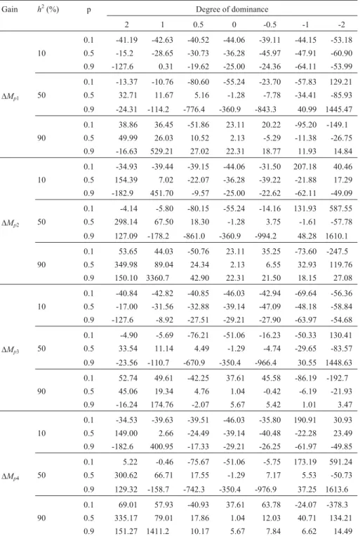
Few experimental studies have compared predicted and realized gains, especially using mass selection. This lack of data makes it difficult to compare the results for bi-ases in gain predictions with mass selection (Table 1). An-other limiting factor, even when experimental data are available, is the lack of knowledge about gene frequencies in the population under selection,i.e., the level of breeding in the population and the degree of dominance of the genes controlling the traits being studied. As shown here, the pre-diction of gain from selection is biased, even when the true values of the genetic parameters (unbiased estimates) are used in the calculation. Ignoring biases > 300% that essen-tially reflected only a small predicted gain and no actual gain, the mean biases in this simulation ranged from 39.2% to 59.3%, depending on the prediction function used.
Ex-treme values generally represented < 10% of the cases and occurred mainly in bred populations with average heri-tability.
Overestimation of gain was not a general rule in our analysis. When additive variance or narrow sense heritability was used there was a tendency to underestimate the gain, particularly with low heritability (Table 1). How-ever, when genotypic variance or broad sense heritability was used, the overestimation of gain for traits with a mean dominance =1.0 was more frequent. Consequently, the use of genotypic variance or broad sense heritability (rather than additive variance and narrow sense heritability) was a further source of bias in gain prediction. In several cases, the bias went from negative (underestimation) to positive (overestimation) values, with an increase in magnitude. The mean absolute values of the biases ranged from 39.2% to 59.3% (increase of 51.3%) with the use of genotypic variance, and from 41.3% to 49.9% (increase of 20.8%) with the use of broad sense heritability. The magnitude and sign of the biases further showed that prediction based on selection intensity and additive variance was equivalent to prediction based on narrow sense heritability and selection differential (means absolute values of the biases were 39.2% and 41.3%, respectively). The same was true for the use of genotypic variance and broad sense heritability (means of 59.3% and 49.9%, respectively).
The results of different traits showed that the magni-tude of the bias was proportional to the degree of domi-nance, regardless of whether the favorable genes were dominant or recessive (Table 1). With prediction based on additive variance, the mean magnitude of the bias with complete dominance/overdominance and partial dominan-ce/absence of dominance was 47.7% and 27.5%, respec-tively. Finally, small magnitude bias was observed in popu-lations with intermediate frequencies and under high heritability conditions. The means of the absolute values were 42.2%, 42.9% and 32.9% for cases of low, medium and high heritability, respectively, and 51.9%, 27.5% and 37.9% in non-bred populations, populations with interme-diate frequencies, and bred populations, respectively, with prediction based on additive variance.
When gain is predicted based on biased estimates of the genetic parameters, the additional bias can increase or decrease the difference between the realized and predicted gains. Using estimates of additive variance (obtained by parent/offspring and mid-parent/offspring regressions) and genotypic variance (obtained from the difference between the phenotypic and environmental variances), the
simula-tion study confirmed almost all of the previous inferences. The exception was a small bias in a bred population, for which the mean magnitude ranged from 27.4% to 47.9%, depending on the prediction function. The bias in the esti-mates of additive variance ranged from -30.1% to 24.6%, with a predominance of underestimation (71.4% of the cases), which explained the smaller magnitude of the bias
Table 1- Percentage bias between realized and predicted gains in the first mass selection cycle based on unbiased estimates of additive and genotypic
variances1.
Gain h2(%) p Degree of dominance
2 1 0.5 0 -0.5 -1 -2
0.1 -41.19 -42.63 -40.52 -44.06 -39.11 -44.15 -53.18 10 0.5 -15.2 -28.65 -30.73 -36.28 -45.97 -47.91 -60.90 0.9 -127.6 0.31 -19.62 -25.00 -24.36 -64.11 -53.99
0.1 -13.37 -10.76 -80.60 -55.24 -23.70 -57.83 129.21
DMp1 50 0.5 32.71 11.67 5.16 -1.28 -7.78 -34.41 -85.93
0.9 -24.31 -114.2 -776.4 -360.9 -843.3 40.99 1445.47
0.1 38.86 36.45 -51.86 23.11 20.22 -95.20 -149.1 90 0.5 49.99 26.03 10.52 2.13 -5.29 -11.38 -26.75
0.9 -16.63 529.21 27.02 22.31 18.77 11.93 14.84
0.1 -34.93 -39.44 -39.15 -44.06 -31.50 207.18 40.46 10 0.5 154.39 7.02 -22.07 -36.28 -39.22 -21.88 17.29 0.9 -182.9 451.70 -9.57 -25.00 -22.62 -62.11 -49.09
0.1 -4.14 -5.80 -80.15 -55.24 -14.16 131.93 587.55
DMp2 50 0.5 298.14 67.50 18.30 -1.28 3.75 -1.61 -57.78
0.9 127.09 -178.2 -861.0 -360.9 -994.2 48.28 1610.1
0.1 53.65 44.03 -50.76 23.11 35.25 -73.60 -247.5 90 0.5 349.98 89.04 24.34 2.13 6.55 32.93 119.76
0.9 150.10 3360.7 42.90 22.31 21.50 18.15 27.08
0.1 -40.84 -42.82 -40.85 -46.03 -42.94 -69.64 -56.36 10 0.5 -17.00 -31.56 -32.88 -39.14 -47.09 -48.18 -58.84 0.9 -127.6 -8.92 -27.51 -29.21 -27.90 -63.97 -54.68
0.1 -4.90 -5.69 -76.21 -51.06 -16.23 -50.33 130.41
DMp3 50 0.5 33.54 11.14 4.49 -1.29 -4.74 -29.65 -83.57
0.9 -23.56 -110.7 -670.9 -350.4 -966.4 30.55 1448.63
0.1 52.74 49.61 -42.25 37.61 45.58 -86.19 -192.7 90 0.5 45.06 19.34 4.76 1.04 -0.42 -6.19 -21.93
0.9 -16.24 174.76 -2.07 5.67 5.42 1.01 3.47
0.1 -34.53 -39.63 -39.51 -46.03 -35.80 190.91 30.93 10 0.5 149.00 2.66 -24.49 -39.14 -40.48 -22.28 23.49 0.9 -182.6 400.95 -17.33 -29.21 -26.25 -61.97 -49.85
0.1 5.22 -0.46 -75.67 -51.06 -5.75 173.19 591.24
DMp4 50 0.5 300.62 66.71 17.55 -1.29 7.17 5.53 -50.73
0.9 129.32 -158.7 -742.3 -350.4 -976.9 37.25 1613.6
0.1 69.01 57.93 -40.93 37.61 63.78 -24.07 -378.3 90 0.5 335.17 79.01 17.86 1.04 12.03 40.71 134.21
0.9 151.27 1411.2 10.17 5.67 7.84 6.62 14.49
1D
Mp1,DMp2,DMp3, andDMp4are the predicted gains based on additive variance, genotypic variance, narrow sense heritability and broad sense
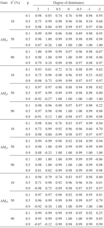
observed here. With few exceptions, the realized and pre-dicted gains during 10 cycles were also in full agreement (average correlation of 0.80).
Half-sib selection
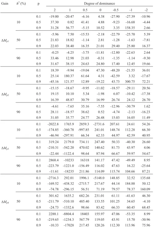
The results of bias in predictions of gain from family selection showed similarities and differences compared to those obtained with mass selection (Table 3). Although the amplitude of the absolute value of bias was not smaller (minimum of 0.25% and maximum of 158.4%, with predic-tion based on the parametric value of the additive variance), there were no very high results (> 300%) and the mean value was 17.7%. The corresponding values in the case of mass selection were 0.31%, 149.1% and 39.2% (Table 1). Although the frequency of cases involving overestimation and underestimation were equivalent (54% and 46%), there was a tendency for overestimation in traits controlled by dominant favorable genes. These results were similar to the findings of Carvalhoet al.(2000) for corn yield, in which the bias between the predicted and realized gains was 287.3%. Bonomo et al. (2000) reported yield biases of 53.5%, 119.0%, 129.8% and 88.3% when the selection in-tensity varied from the lowest to the highest value. More re-cently, Viana (2007) calculated the realized gain by using the means of the progeny tests and observed full correspon-dence between the realized and predicted gains. The re-spective means of the predicted and realized gains for the three selection cycles were 5.6% and 5.6% for expansion volume, and 8.1% and 7.8% for yield.
The mean absolute values of biases by trait, popula-tion and heritability were larger with complete dominance and overdominance (21.4%), in bred populations (28.9%) and with low heritability (23.8%) (Table 3). The mean val-ues in cases of partial/absence of dominance, in non-bred populations and in populations with intermediate gene fquencies, average heritability and high heritability were, re-spectively, 12.7%, 12.3%, 11.9%, 14.7% and 14.6%. Once again, equivalence was observed between prediction based on selection intensity and additive variance and prediction based on narrow sense heritability and selection differen-tial. For bias in the predictions based on estimates of addi-tive variance, all of the previous inferences were con-firmed, with no exceptions (Table 3). Although the use of biased estimates of genetic parameters can either increase or decrease the bias calculated based on parametric values, only increases were observed here. The absolute minimum, mean and maximum values were 0.52%, 25.9% and 180.4%, respectively.
The gain prediction from family selection was a poorer indicator of the efficiency of recurrent population breeding methods and selection strategies compared to similar prediction from mass selection (Table 4). The linear association between predicted and realized gains during 10 cycles was only adequate for heritability > 50%, regardless of the traits and the bias in the additive variance estimates.
The mean correlation was 0.71 for prediction based on un-biased estimates of the additive variance, and 0.59 in the case of prediction based on biased estimates. When low heritability cases were excluded, the mean correlations were 0.85 and 0.81.
Table 2- Correlation between realized and predicted gains in 10 mass
se-lection cycles based on unbiased estimates of additive and genotypic vari-ances1.
Gain h2(%) p Degree of dominance
2 1 0.5 0 -0.5 -1 -2
0.1 0.98 0.85 0.74 0.76 0.98 0.98 0.95 10 0.5 0.75 0.99 0.90 0.96 0.96 0.54 0.68 0.9 0.98 0.80 0.99 0.99 0.97 0.97 0.96
0.1 0.99 0.99 0.96 0.88 0.89 0.98 0.95
DMp1 50 0.5 0.98 1.00 0.99 0.99 0.98 0.98 0.98
0.9 0.87 -0.26 1.00 1.00 1.00 1.00 1.00
0.1 1.00 0.99 0.99 0.97 0.96 0.98 -0.07 90 0.5 0.98 1.00 0.99 1.00 0.99 0.98 0.96 0.9 0.79 0.18 0.99 0.98 0.97 0.98 0.97
0.1 0.93 0.81 0.72 0.76 0.98 0.99 0.82 10 0.5 0.75 0.98 0.90 0.96 0.95 0.53 -0.02 0.9 -0.98 0.75 0.99 0.99 0.97 0.97 0.97
0.1 0.97 0.97 0.96 0.88 0.94 0.98 0.82
DMp2 50 0.5 0.97 0.99 0.99 0.99 0.98 0.98 0.80
0.9 -0.92 -0.27 1.00 1.00 1.00 1.00 1.00
0.1 0.98 0.96 0.98 0.97 0.97 0.98 0.22 90 0.5 0.97 0.98 0.98 1.00 1.00 0.99 0.88 0.9 -0.91 0.13 1.00 0.98 0.97 0.99 0.98
0.1 0.98 0.84 0.76 0.83 0.97 0.99 0.94 10 0.5 0.73 0.99 0.92 0.96 0.96 0.60 0.70 0.9 0.98 0.80 0.99 0.98 0.97 0.97 0.97
0.1 0.99 0.99 0.98 0.92 0.94 0.99 0.94
DMp3 50 0.5 0.98 1.00 0.99 0.99 0.99 0.99 0.99
0.9 0.88 -0.33 1.00 1.00 0.99 1.00 1.00
0.1 1.00 1.00 1.00 0.99 0.99 0.99 -0.06 90 0.5 0.98 1.00 0.99 1.00 1.00 0.99 0.98 0.9 0.81 0.02 0.99 0.98 0.99 0.99 0.98
0.1 0.94 0.79 0.74 0.83 0.97 0.98 0.80 10 0.5 0.71 0.98 0.92 0.96 0.96 0.56 0.01 0.9 -0.98 0.75 0.99 0.98 0.97 0.97 0.97
0.1 0.97 0.97 0.98 0.92 0.98 0.95 0.81
DMp4 50 0.5 0.96 0.99 0.99 0.99 0.99 0.97 0.79
0.9 -0.92 -0.38 1.00 1.00 0.99 1.00 1.00
0.1 0.99 0.99 0.99 0.99 0.95 0.92 0.25 90 0.5 0.95 0.99 0.99 1.00 1.00 0.99 0.85 0.9 -0.87 -0.12 0.99 0.98 0.99 0.99 0.99
1D
Mp1,DMp2,DMp3, andDMp4are the predicted gains based on additive
Comparison of the predicted and realized gains based on the selection of individuals in the best families yielded poor results (Tables 3 and 4). In approximately 54% of the cases, the realized gain was practically nil, implying very high bias values in relation to the predicted gain (Table 3). This situation occurred in predictions of traits controlled by
dominant favorable genes (degree of dominance > 0, re-gardless of the bias in the estimates of additive variance). When these values were ignored, the smallest magnitude of bias was 4.6% and the absolute maximum value was 297.9%, with prediction using unbiased estimates of addi-tive variance. The mean magnitude of the bias was 94.5%.
Table 3- Percentage bias between realized and predicted gains in the first half-sib selection cycle based on unbiased and biased estimates of additive
vari-ance1.
Gain h2(%) p Degree of dominance
2 1 0.5 0 -0.5 -1 -2
0.1 -19.00 -20.47 -6.16 4.38 -27.90 -27.39 -10.96 10 0.5 37.30 0.82 41.41 4.88 -9.23 -16.68 -4.44 0.9 31.28 56.77 -5.15 10.52 3.35 158.35 2.66
0.1 -5.96 7.50 -15.53 -2.18 -22.79 -25.70 5.39
DMp1 50 0.5 21.83 18.82 -1.14 2.81 -1.28 -1.63 -7.81
0.9 22.03 38.40 16.35 21.01 29.40 25.80 16.37
0.1 -0.25 -4.25 -3.75 -11.81 -12.80 -22.63 2.64 90 0.5 33.46 12.98 21.03 -0.31 -1.35 -1.14 -9.30 0.9 31.67 38.15 24.63 24.80 17.40 12.45 19.66
0.1 18.39 -9.94 -19.04 47.30 -48.20 -21.55 36.01 10 0.5 25.14 180.37 61.64 4.31 -42.59 3.32 -17.67 0.9 -45.16 121.57 12.89 -19.22 43.73 300.75 72.21
0.1 -15.15 -18.67 -9.95 -11.02 -18.57 -29.11 20.56
DMp2 50 0.5 19.15 10.10 5.34 -1.98 6.07 -10.42 -17.38
0.9 16.39 48.87 30.79 16.99 26.74 24.12 26.70
0.1 -4.61 -7.65 35.16 -7.55 -12.96 -30.79 1.62 90 0.5 28.11 -18.57 38.62 0.52 -4.74 -2.13 -16.23 0.9 31.05 35.77 24.77 26.48 15.03 16.05 11.49
0.1 -2022.8 1765.9 2859.3 -2731.6 207.61 24.61 54.26 10 0.5 -174.85 -360.78 -997.85 241.01 148.74 112.28 66.30 0.9 -46.94 -297.91 66.34 62.33 44.97 42.59 40.95
0.1 319.24 2179.0 734.11 247.40 50.33 -40.30 26.60
DMp3 50 0.5 -210.31 -542.20 470.02 140.62 81.73 43.97 4.06
0.9 -22.44 -1122.4 98.64 87.94 66.67 59.97 54.67
0.1 2868.4 -10233 16318 141.17 47.42 -49.49 8.95 90 0.5 -223.79 -1221.0 -156.49 116.02 47.63 16.22 -25.64 0.9 -11.61 -18235 211.86 114.09 115.74 104.66 87.21
0.1 -2716.3 292.01 1996.1 -5148.0 148.85 32.52 135.68 10 0.5 -169.52 -438.32 -2715.7 217.67 44.14 184.88 50.12 0.9 -74.78 -296.15 56.51 71.19 79.57 78.37 160.09
0.1 301.62 1635.2 682.26 231.01 61.11 -41.63 46.30
DMp4 50 0.5 -211.79 -510.10 485.40 133.55 101.25 34.65 -4.10
0.9 -24.73 -1332.6 98.66 83.42 66.33 60.45 68.45
0.1 2288.1 -8804.4 18403 155.97 47.06 -53.35 8.99 90 0.5 -219.65 -1234.3 567.79 119.05 43.91 15.70 -30.96 0.9 -10.33 -17028 217.45 120.26 112.30 113.96 75.96
1DM
p1andDMp2are the predicted gains with family selection, calculated based on the parametric and estimated values of additive variance;DMp3and DMp4are the predicted gains with selection of individuals in the best progenies, calculated based on the parametric and estimated values of additive
These values were greater than those observed with mass selection, indicating that prediction of gain from within half-sib selection is more biased than prediction of gain
from mass selection using unbiased estimates of additive variance. There was a tendency for underestimation in traits controlled by favorable genes with a degree of dominance > 1.0, as also seen with corn grain yield. However, overesti-mation was detected in the other situations. These observa-tions agreed with findings for popcorn yield (Matta and Viana, 2003), for which the biases in gain predictions from among and within selection were 218.1% and -116.3%, re-spectively, in line with the theoretical results. For expan-sion volume, considered by Scapim et al. (2002) to be determined by favorable dominant and recessive genes (bi-directional dominance), the bias was towards underesti-mation, i.e., -18.4% with progeny selection and -78.4% with selection of individuals in the selected families. As ex-pected, bias in gain prediction from within selection was much larger than bias in gain prediction from among family selection.
Greater biases were observed for traits controlled by favorable dominant genes (average magnitudes of 133.3%, 297.9% and 115.0% for degrees of dominance of 0.5, 1 and 2, respectively) and traits not controlled by allelic interac-tion effects (average magnitude of 143.8%) (Table 3). The average absolute values of the biases for traits controlled by favorable recessive genes were 90.1%, 54.9% and 41.0% for degrees of dominance of -0.5, -1 and -2, respectively. Greater absolute biases were observed in populations with intermediate gene frequencies (113.1% versus 81.6% and 86.2%, in non-bred and bred populations) and low heri-tability (108.8% versus 82.4% and 92.4%, with medium and high heritability). The predicted gains calculated based on biased estimates of additive variance were more biased, but generally confirmed the results obtained by using the parametric value. The minimum, mean and maximum mag-nitudes were 4.1%, 102.3% and 296.1%, respectively.
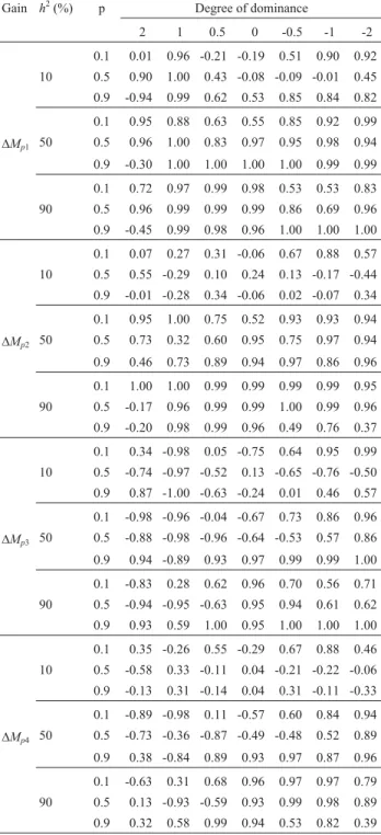
An additional negative aspect of gain prediction from individual selection within the selected families was shown by the correlation between predicted and realized gain dur-ing 10 cycles. Regardless of the magnitude of the bias in ad-ditive variance, the correlation was negative in ~40% of the situations assessed (Table 4) but was > 0.7 in only 30%-40% of the cases. Only in cases of traits controlled by favorable recessive genes with average to high heritability was there sufficient agreement between predicted and real-ized gains to allow assessment of the efficiency of the re-current breeding method and selection strategies (average correlation of 0.75, regardless of the bias in the additive variance estimate). The average correlations for unbiased and biased estimates of the additive variance were 0.15 and 0.24, respectively.
In conclusion, the use of unbiased and biased esti-mates of the genotypic variance within progeny rather than the within family additive variance,i.e., broad versus nar-row sense heritability, increased the magnitude of bias without worsening the correlation between predicted and realized gains. These findings indicate that Eberharts
for-Table 4- Correlation between realized and predicted gains during 10 half-sib selection cycles based on unbiased and biased estimates of addi-tive variance1.
Gain h2(%) p Degree of dominance
2 1 0.5 0 -0.5 -1 -2
0.1 0.01 0.96 -0.21 -0.19 0.51 0.90 0.92 10 0.5 0.90 1.00 0.43 -0.08 -0.09 -0.01 0.45 0.9 -0.94 0.99 0.62 0.53 0.85 0.84 0.82
0.1 0.95 0.88 0.63 0.55 0.85 0.92 0.99
DMp1 50 0.5 0.96 1.00 0.83 0.97 0.95 0.98 0.94
0.9 -0.30 1.00 1.00 1.00 1.00 0.99 0.99
0.1 0.72 0.97 0.99 0.98 0.53 0.53 0.83 90 0.5 0.96 0.99 0.99 0.99 0.86 0.69 0.96 0.9 -0.45 0.99 0.98 0.96 1.00 1.00 1.00
0.1 0.07 0.27 0.31 -0.06 0.67 0.88 0.57 10 0.5 0.55 -0.29 0.10 0.24 0.13 -0.17 -0.44 0.9 -0.01 -0.28 0.34 -0.06 0.02 -0.07 0.34
0.1 0.95 1.00 0.75 0.52 0.93 0.93 0.94
DMp2 50 0.5 0.73 0.32 0.60 0.95 0.75 0.97 0.94
0.9 0.46 0.73 0.89 0.94 0.97 0.86 0.96
0.1 1.00 1.00 0.99 0.99 0.99 0.99 0.95 90 0.5 -0.17 0.96 0.99 0.99 1.00 0.99 0.96 0.9 -0.20 0.98 0.99 0.96 0.49 0.76 0.37
0.1 0.34 -0.98 0.05 -0.75 0.64 0.95 0.99 10 0.5 -0.74 -0.97 -0.52 0.13 -0.65 -0.76 -0.50 0.9 0.87 -1.00 -0.63 -0.24 0.01 0.46 0.57
0.1 -0.98 -0.96 -0.04 -0.67 0.73 0.86 0.96
DMp3 50 0.5 -0.88 -0.98 -0.96 -0.64 -0.53 0.57 0.86
0.9 0.94 -0.89 0.93 0.97 0.99 0.99 1.00
0.1 -0.83 0.28 0.62 0.96 0.70 0.56 0.71 90 0.5 -0.94 -0.95 -0.63 0.95 0.94 0.61 0.62 0.9 0.93 0.59 1.00 0.95 1.00 1.00 1.00
0.1 0.35 -0.26 0.55 -0.29 0.67 0.88 0.46 10 0.5 -0.58 0.33 -0.11 0.04 -0.21 -0.22 -0.06 0.9 -0.13 0.31 -0.14 0.04 0.31 -0.11 -0.33
0.1 -0.89 -0.98 0.11 -0.57 0.60 0.84 0.94
DMp4 50 0.5 -0.73 -0.36 -0.87 -0.49 -0.48 0.52 0.89
0.9 0.38 -0.84 0.89 0.93 0.97 0.87 0.96
0.1 -0.63 0.31 0.68 0.96 0.97 0.97 0.79 90 0.5 0.13 -0.93 -0.59 0.93 0.99 0.98 0.89 0.9 0.32 0.58 0.99 0.94 0.53 0.82 0.39
1D
Mp1andDMp2are the predicted gains with family selection, calculated
based on the parametric and estimated values of additive variance;DMp3
andDMp4are predicted gains with selection of individuals in the best
mula, which is a function of additive variance or narrow sense heritability, is a less biased estimator of genetic gain than the estimator based on a function of genotypic vari-ance or broad sense heritability. As shown for mass and family selection, there was full correspondence between the gains calculated with additive or genotypic variance and the predictions based on broad or narrow sense heri-tability.
References
Baltunis BS, Huber DA, White TL, Goldfarb D and Stelzer HE (2007) Genetic gain from selection for rooting ability and early growth in vegetatively propagated clones of loblolly pine. Tree Genet Genomes 3:227-238.
Bonomo P, Sampaio NF, Viana JMS and Oliveira AB (2000) Comparação entre ganhos preditos e realizados na produção de grãos da população de milho Palha Roxa. Rev Ceres 47:383-392.
Bordes J, Charmet G, Vaulx RD, Pollacsek M, Beckert M and Gallais A (2006) Doubled haploid versus S1family recurrent
selection for testcross performance in a maize population. Theor Appl Genet 112:1063-1072.
Carvalho WHL and Souza EM (2007) Ciclos de seleção de progê-nies de meios-irmãos do milho BR 5011 Sertanejo. Pesq Agropec Bras 42:803-809.
Carvalho HWL, Guimarães PEO, Leal MLS, Carvalho PCL and Santos MX (2000) Avaliação de progênies de meios-irmãos da população de milho CMS-453 no nordeste brasileiro. Pesq Agropec Bras 35:1577-1584.
Eberhart SA (1970) Factors effecting efficiencies of breeding methods. Afr Soils 15:669-680.
Falconer DS (1960) Introduction to Quantitative Genetics. Ron-ald, New York, 365 pp.
Gonçalves GM, Viana AP, Neto FVB, Pereira MG and Pereira TNS (2007) Seleção e herdabilidade na predição de ganhos genéticos em maracujá-amarelo. Pesq Agropec Bras 42:193-198.
Hallauer AR and Miranda Filho JB (1988) Quantitative Genetics in Maize Breeding. 2nd edition. Iowa State University Press, Ames, 468 pp.
Loywyck V, Bijma P, van der Laan MHP, van Arendonk J and Verrier E (2005) A comparison of two methods for predic-tion of response and rates of inbreeding in selected popula-tions with the results obtained in two selection experiments. Genet Sel Evol 37:273-289.
Matta FP and Viana JMS (2003) Eficiências relativas dos proces-sos de seleção entre e dentro de famílias de meios-irmãos em população de milho-pipoca. Ciênc Agrotecnol 27:548-556. Rose LW, Das MK, Fuentes RG and Taliaferro CM (2007) Effects
of high- vs. low-yield environments on selection for in-creased biomass yield in switchgrass. Euphytica 156:407-415.
Scapim CA, Pacheco CAP, Tonet A, Braccini AL and Pinto RJB (2002) Análise dialélica e heterose de populações de milho-pipoca. Bragantia 61:219-230.
Viana JMS (2007) Melhoramento intrapopulacional recorrente de milho-pipoca, com famílias de meios-irmãos. Rev Bras Mi-lho Sorgo 6:199-210.
Wricke G and Weber WE (1986) Quantitative Genetics and Selec-tion in Plant Breeding. Walter de Gruyter, Berlin, 406 pp.
Associate Editor: Pedro Franklin Barbosa