Elastic Cross Sections for Low-Energy e ,
{CH 4
Collisions L. E. Machado
1
, M.-T.Lee 2
and L. M. Brescansin 3 1 Departamento de Fsica, UFSCar, 13565-905, S~ao Carlos, SP, Brazil 2 Departamento de Qumica, UFSCar, 13565-905, S~ao Carlos, SP, Brazil 3
Instituto de Fsica \Gleb Wataghin", UNICAMP, 13083-970, Campinas, SP, Brazil
ReceivedFebruary12,1998
Recently we have extended our codes based on the Schwinger variational iterative method in order to study elastic electron scattering by non-planar molecules with symmetries reducible to the C2v point group and also to include a correlation-polarization contribution to the electron-molecule interaction potential. In this work we report the rst application of these newly extended codes to the calculation of cross sections for low-energy elastic scattering of electrons by methane. Dierential, integral and momentum-transfer cross sections were calculated in the 0.1{50 eV incident energy range. Comparison of our results with the extensive available data, both experimental and theoretical, reveals the reliability of our method. Particularly, the Ramsauer minimumat around 0.4 eV and the resonance structure at around 8 eV are well reproduced in our calculations.
I. Intro duction
Over the last fteen years the Schwinger variational iterative method (SVIM) [1] has been widely used for calculations on elastic electron-molecule scattering [2-6] and molecular photoionization [1, 7-11]. Also, com-bined with the distorted-wave approximation, SVIM has been applied to the investigation of electronic ex-citation in molecules [12-18]. Besides its capability of treating electron scattering by both neutral and ionic molecular targets, SVIM has very solid theoretical grounds. It provides continuum wavefunctions that are shown to converge to the exact solutions of the spec-ied projectile-target interaction potential being used [19]. Fully ab-initiocalculations using SVIM have led to reliable cross sections and other related parameters over a large range of incident energies, from low (a few eV) to intermediate (up to a hundred eV) in a number of previous applications. However, except for a study on photoionization of methane [10] the use of SVIM has been limited to diatomic, linear and planar polyatomic molecular targets. In addition, those applications of the method have been restricted to the static-exchange (SE) level of approximation. On the other hand,
accu-rate descriptions of the electron-molecule collision dy-namics at the low and very-low (sub-eV) energy ranges usually require treatments beyond the SE level of ap-proximation, namely, an appropriate balance of static, exchange and correlation-polarization potentials. We have recently extended our SVIM codes in order to treat nonplanar molecules with symmetry reducible to C2v. Also, in this extended version a local correlation-polarization contribution to the electron-molecule inter-action potential is included, following the prescription recommended by Padial and Norcross [20]. As a rst application of the new version of our codes we studied the elastice
,{CH
4scattering in a wide incident energy range.
30's showed a deep minimum at around 0.4 eV and a broad maximum at 8 eV in the total cross sections [24-27]. These structures have also been seen in more re-cent measurements of elastic integral and momentum-transfer cross sections (ICS and MTCS) [28-34]. Dif-ferential cross sections (DCS) of elastically scattered electrons have also been extensively studied. Recent experimental data on DCS were reported in a number of works: Curryetal. [21], Tanakaetal. [28], Vuskovic and Trajmar [29], Sohn et al. [30], Shyn and Cravens [31], Boesten and Tanaka [32], Kanik et al. [33] and Mapstone and Newell [35], just to cite a few.
On the theoretical side, the literature is equally rich. DCS, MTCS as well as ICS for elastic e
,{CH 4 scat-tering have been calculated in the last fteen years at dierent levels of approximation. Model poten-tials at static-exchange (SE) and at static-exchange-polarization (SEP) levels were used by several authors [36-39]. The Schwinger multichannel method using pseudopotentials was applied by Bettega etal. [40] to study elastic scattering of electrons by XH4 molecules (X=C, Si, Ge, Pb). An exact SE calculation for elastic e,{CH
4 scattering was reported by Lima
et al. [41]. Beyond the exact-SE level, the correlation-polarization contributions to the interaction potential were taken into account either via an approximated local function [42,43] or via a multichannel treatment of the scattering equations [44,45].
In this work we use our newly extended version of the SVIM codes to calculate DCS, ICS and MTCS for elastic e
,{CH
4 scattering in the 0.1{50 eV energy range. The large amount of data provided by this cal-culation will be compared with the numerous results available in the literature. Our particular interest is to check if our method is capable, for instance, of describ-ing correctly the structures in the ICS curve, namely, the Ramsauer minimum at very low energies and the broad resonance at around 8 eV. Once the reliability is rmly assured, our new codes will be applied to electron scattering by larger nonplanar systems.
The organization of the paper is as follows. In Sec. II we briey discuss some aspects of the theory been used and in Sec. III we present some details of the computation. Our results are presented and compared with the available data in the literature in Sec. IV, where we also present short concluding remarks.
I I. Theory andcalculation
The Schrodinger equation for the continuum scat-tering orbitals can be written (in atomic units) as:
,r
2+
U(~r),k 2
~k(~r) = 0 (1) where U(~r) = 2V(~r) and V(~r) is the interaction po-tential between the target and the scattering electron. Eq. (1) can be converted into an equivalent Lippmann-Schwinger equation
()
~k = ~k+G () 0
U ()
~k (2)
withG ()
0 being the free-particle Green's operator with outgoing- (G
(+)
0 ) or incoming-wave ( G
(,)
0 ) boundary conditions. In order to take advantage of the symme-try of the target, the scattering wavefunctions can be partial-wave expanded as:
()
~k (~r) = h
2 i
1 21
k X
plh
il ()
p
k;lh (~r)X
p
lh (^k): (3) where Xlhp(^r) are generalized spherical harmonics, re-lated to the usual spherical harmonicsYlm by:
Xlhp(^r) = X
m
bplhmYlm(^r): (4) Here p is an irreducible representation (IR) of the molecular point group,is a component of this repre-sentation andhdistinguishes between dierent bases of the same IR corresponding to the same value ofl. The coecients b
p
T () ~ k ; ~ k0 = < () ~ k
jU j ~ () ~ k0
>+< ~ () ~ k
jU j () ~ k0 >, < ~ () ~ k
jU,UG () 0
U j ~ () ~ k 0
> (5)
with ~ () ~
k denoting trial scattering wavefunctions . Using partial-wave expansions similar to (3) for both ~ () ~ k and the free-particle wave vector ()
~
k , a partial wave on-shell T matrix (diagonal in both
pand) is obtained: T () p k ;lh;l 0 h 0 = < () p k ;l 0 h 0
jU j ~ ()
p k ;lh
>+< ~ () p k ;l 0 h 0
jU j () p k ;lh >, < ~ () p k ;l 0 h 0
jU,UG () 0
U j ~ ()
p k ;lh
> (6)
where k = j ~ k 0
j = j ~
kjfor the elastic process.
The initial scattering wave functions can be expanded in a set R 0 of
L
2basis functions
i(
~r) =<~rj i
>: ~ ()
p k ;lh (
~ r) =
N X i=1 a () p i;lh ( k) i( ~
r) (7)
Using (6) and (7), variationalT ()
p k ;lh;l
0 h
0 matrix elements can be derived as: T () p k ;lh;l 0 h 0 = N X i;j=1 < () p k ;l 0 h 0
jU j i
>[D ()
,1 ]ij
< j
jU j () p k ;lh > (8) where D () ij = < i
jU ,UG () 0
U j j
> (9)
and the corresponding approximate scattering solution with outgoing-wave boundary condition becomes:
(+) p
(S 0
) k ;lh (
~r) = p k ;lh(
~r) + M X i;j=1
<~rjG (+) 0
U j i
>[D (+)
,1 ]ij
< j
jU j p k ;lh
> (10)
Converged outgoing solutions of (2) can be obtained via an iterative procedure. The method consists in augmenting the basis set R
0by the set S 0 = f (+) p (S 0 ) k ;l1h1 (
~r); (+)
p (S
0 ) k ;l2h2 (
~r);::: (+)
p (S
0 ) k ;lchc (
~
r)g (11)
where l
c is the maximum value of
l for which the expansion of the scattering solution (3) is truncated. A new set of partial wave scattering solutions can now be obtained from:
(+) p
(S 1
) k ;lh (
~r) = p k ;lh(
~ r) +
M X i;j=1
<~rjG (+)
U j (S0) i
>[D (+) ,1 ]ij < (S0) j
jU j p k ;lh > (12) where (S 0 ) i ( ~
r) is any function in the setR 1=
R 0
S S
0 and M is the number of functions in R
1. This iterative pro-cedure continues until a converged (+)
p (S
n ) k ;lh (
~
r) is achieved. These converged scattering wavefunctions correspond, in fact, to exact solutions of the truncated Lippmann-Schwinger equation with the potentialU.
In an actual calculation we compute the converged partial wave K-matrix elements,K p
(Sn) k ;lh;l
0 h
0. These K-matrix elements can be obtained by replacing D
(+) by its principal value, D
(P), in Eq. (8). Hence, the corresponding partial-wave T-matrix elements can be calculated from
T p (S n ) k ;lh;l 0 h 0 = , h 2 i X [1,iK
By usual transformations, these matrix elements can be expressed in the laboratory frame (LF). The LF scattering amplitude f(^k0;^k0
0) is related to the T matrix by: f(^k0; ^k0
0) = ,2
2T; (14)
where ^k0 0 and ^k
0are the directions of incident and scattered electron linear momenta, respectively. The dierential cross section for elastic electron-molecule scattering is given by:
d
d = 812 Z
dsinddjf(^k 0;^k0
0) j
2: (15)
Here, (, , ) are the Euler angles which dene the orientation of the principal axes of the molecule. Finally, after some angular momentum algebra, the LF DCS averaged over the molecular orientations can be written as:
d d =
X
L AL(k)PL(cos) (16)
where is the scattering angle. The coecients AL(k) in Eq. (16) are given by the formula AL(k) = 122L + 11
X
plhl0h0mm0
p11l1h1l 0 1h 0 1m 1m 0 1
(,1)m 0
,m p
(2l + 1)(2l1+ 1) bp11
l0 1h 0 1m 0 1
bp11
l1h1m1b
p
l0h0m0b
p lhmap1
1
l1h1;l 0 1h
0 1
(k)aplh;l0h0(k)
(17)
(l10l0 jL0)(l 0 10l 00 jL0)(l 1 ,m 1lm
jL,M)(l 0 1m
0 1l
0m0 jLM) where (j1m1j2m2
j j
3m3) are the usual Clebsch-Gordan coecients and the auxiliary amplitudes a
p
lh;l0h0(k) are dened as
aplh;l0h0(k) = ,
p 3 k il
0 ,l
p
2l0+ 1Tp (Sn)
k;lh;l
0h0: (18)
d
III. Computational details
In our study U is an optical potential which includes both an exact static-exchange part and a parameter-free correlation-polarization (CP) contribution. Fol-lowing the prescription of Padial and Norcross [20], the correlation-polarization eects are introduced in the po-tential through a parameter-free model which combines the target correlation calculated from the local electron-gas theory for short distances with the asymptotic form of the polarization potential, given (for Td molecules) by:
vp(~r) =, 1 20
r4; (19)
where 0 is the spherical part of the molecular dipole polarizability. In our calculations the experimental value 0= 17:5 a.u. was taken [47]. An SCF wavefunc-tion for methane ground state is obtained and is used
to generate the static-exchange-polarization potential. In Table 1 we show the contracted Cartesian Gaussian basis set used in this calculation. At the equilibrium C,H bond distance (RC
,H = 2:0503 a0) this basis set gives an SCF energy of -40.1987 a.u. which can be compared with the -40.2155 a.u. value of Nishimura and Itikawa [39]. In the present calculation the cuto parameter used in the expansions of the target bound orbitals and of the static plus CP potential is lc = 16. All possible values of h l are retained. With this cuto, the normalization of all bound orbitals is better than 0.999. In SVIM calculations, we have limited the partial-wave expansions to lc= 12 for energies E0
Table 1: Cartesian gaussian functions used in the SCF calculations.
Atom s p d
Exp. Coe. Exp. Coe. Exp. Coe.
4232.61 0.006228 18.1557 0.039196 634.882 0.047676 3.98640 0.244144 146.097 0.231439 1.14290 0.816775 42.4974 0.789108
C 14.1892 0.791751 1.96660 0.321870
5.14770 1.000000 0.35940 1.000000 1.500 1.000000 0.49620 1.000000 0.11460 1.000000 0.750 1.000000 0.15330 1.000000 0.04584 1.000000 0.300 1.000000 0.06132 1.000000 0.02000 1.000000
33.6444 1.000000 1.00000 1.000000 5.05796 1.000000 0.50000 1.000000 H 1.14680 1.000000 0.10000 1.000000
0.321144 1.000000 0.101309 1.000000
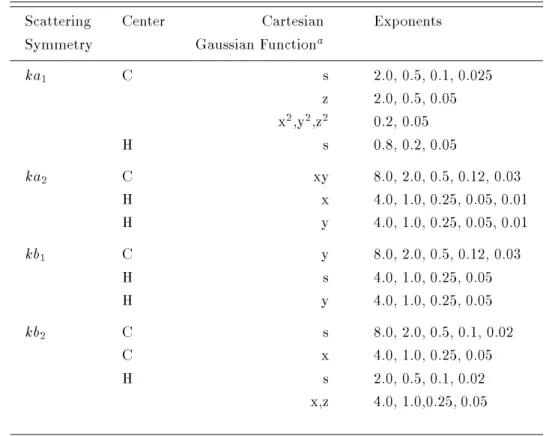
Table 2: Basissetused for the initialscatteringfunctions.
Scattering Center Cartesian Exponents
Symmetry Gaussian Functiona
k a
1 C s 2.0, 0.5, 0.1, 0.025
z 2.0, 0.5, 0.05 x2,y2,z2 0.2, 0.05
H s 0.8, 0.2, 0.05
k a
2 C xy 8.0, 2.0, 0.5, 0.12, 0.03
H x 4.0, 1.0, 0.25, 0.05, 0.01
H y 4.0, 1.0, 0.25, 0.05, 0.01
k b
1 C y 8.0, 2.0, 0.5, 0.12, 0.03
H s 4.0, 1.0, 0.25, 0.05
H y 4.0, 1.0, 0.25, 0.05
k b
2 C s 8.0, 2.0, 0.5, 0.1, 0.02
C x 4.0, 1.0, 0.25, 0.05
H s 2.0, 0.5, 0.1, 0.02
x,z 4.0, 1.0,0.25, 0.05
aCartesian Gaussian basis functions are dened as :
;`;m;n; A(
IV. Resultsanddiscussions
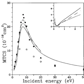
In Figs. 1 and 2 we present our calculated ICS and MTCS, respectively, for elastic e
,{CH
4 scattering, in the 1{50 eV energy range. The insets in both gures show the respective cross sections in the very low en-ergy region. Some selected experimental data and the theoretical results of Jain [36] and of McNaugthen et al. [42] are also shown for comparison. In general, there is a good agreement among the various ICS data. Our calculation has predicted a shape resonance in ICS at around 10 eV which is in good agreement with the theoretical results of Jain [36], though shifted approxi-mately 2 eV from the experimental value. In addition, our calculated Ramsauer minimumis located at around 0.4 eV, slightly lower than the experimental minimum at 0.6 eV. As it can be seen in Fig. 2, all the calcu-lated MTCS agree quite well with each other within 15% and also with the experimental data of Boesten and Tanaka [32]. However, the measured data of Shyn and Cravens [31] are much lower, particularly in the region of the maximum, located at around 8 eV. Our theoretical results also show a minimum in the MTCS at around 0.3 eV which is in very good agreement with both calculated results.
Figure 1: ICS for elastice ,{CH
4 collision in the 0.1-50 eV
energy range. Solid line, present results; dotted line, the-oretical results of Jain (Ref. 36); short-dashed line, theo-retical results of McNaughten et al. (Ref. 42); full circles,
experimental data of Boesten and Tanaka (Ref. 32); full squares, experimental data of Sohnet al. (Ref. 30); open
triangles, experimental data of Vuskovic and Trajmar (Ref. 29). Same symbols are used in the inset.
Figure 2: MTCS for elastic e ,{CH
4 collision. Symbols are
the same as in gure 1, except: open circles, experimental data of Shyn and Cravens (Ref. 31).
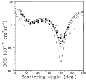
Figure 3: DCS for elastic e ,{CH
4 collision at 0.5 eV. Solid
line, present results ; short-dashed line, theoretical results of Gianturco etal. (Ref. 43); dashed line, theoretical results
of Lengseld III et al. (Ref. 44); long-dashed line,
theo-retical results of Nestmann et al. (Ref. 45); full squares,
experimental data of Sohnetal. (Ref. 30).
In Fig. 3 we show our calculated DCS for elastic
e ,{CH
[30] as well as with some recent theoretical results [42-44]. The deep minimum at 60o in the measured data is fairly well reproduced by the calculations. Neverthe-less, the R-matrix calculation has also shown a second minimum at around 110o, neither seen in the measured nor in all other theoretical data. Quantatively, our cal-culated results are also in general good agreement with the experimental data, particularly for scattering angles above 70o.
In Fig. 4 our calculated DCS at 1.0 eV are com-pared with the experimental data of Sohn et al. [30] and the theoretical results from Jain [36], McNaughten
et al. [42] and Lengseld III et al. [44]. Our calcu-lated SE results are also included in this gure. Again, the deep minimum at around 35o in the experimental data is well reproduced by all calculations which include polarization eects. In particular, our static-exchange plus correlation-polarization calculation shows a very good agreement with the experimental results at the region of the minimum. As expected, the SE calcula-tion was unable to reproduce this feature.
Figure 4: DCS for elastic e ,{CH
4 collision at 1.0 eV. Solid
line, present results; dotted line, theoretical results of Jain (Ref. 36); short-dashed line, theoretical results of Mc-Naughten etal. (Ref. 42) ; dashed line, theoretical results
of Lengseld III etal. (Ref. 44); long-dashed line, present
results, static-exchange approximation; full squares, exper-imental data of Sohn etal. (Ref. 30).
Figures 5-8 show our calculated DCS for elastice ,{ CH4 scattering at 5, 10, 20 and 50 eV, respectively,
along with some available experimental [21, 28-32, 35] and theoretical [36, 39, 41-45] results. In general our calculated DCS agree very well with the measured data both qualitatively and quantitatively, except at 50 eV, where the quantitative agreement is only reasonable. The agreement with other theoretical results is also quite good.
Figure 5: DCS for elastice ,{CH
4collision at 5.0 eV.
Sym-bols are the same as in gure 3, except: full cirles, experi-mental data of Boesten and Tanaka (Ref. 32); open circles, experimental data of Shyn and Cravens (Ref. 31); open squares, experimental data of Tanakaetal. (Ref. 28); full
stars, experimental data of Mapstone and Newell (Ref. 35).
Figure 6: DCS for elastice ,{CH
4collision at 10.0 eV. Solid
line, present results; short-dashed line, theoretical results of McNaughten etal. (Ref. 42); dashed line, theoretical
re-sults of Bettegaetal. (Ref. 40); long-dashed line,
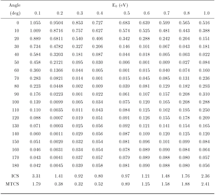
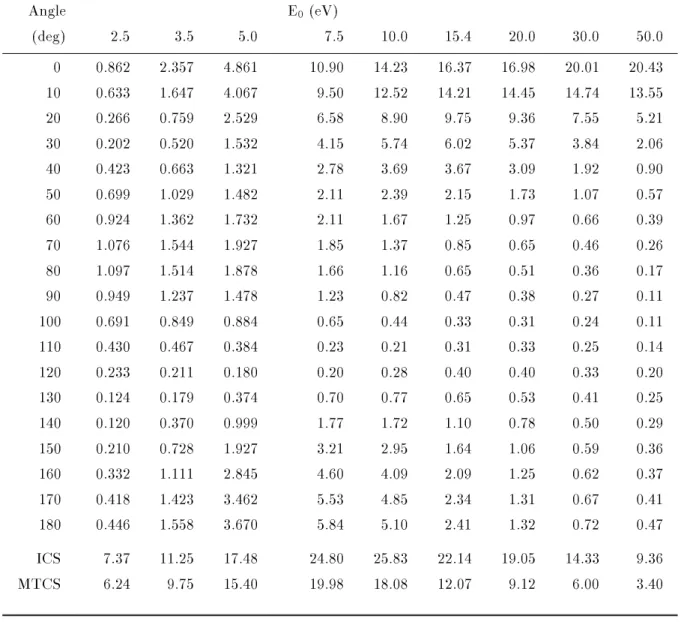
For the sake of completeness, in Table 3 we also present our calculated DCS, ICS, and MTCS for ener-gies ranging from 0.1 to 50 eV.
In summary, the newly extended version of the SVIM codes which accounts for the correlation-polarization eects is applied by the rst time to study the elastic electron scattering by a nonplanar molecule. More especically, we have calculated ICS, MTCS and
DCS for elastice ,{CH
4scattering, over a wide range of incident electron energies. In general our calculated re-sults are in very good agreement with experimental and theoretical data reported in the literature which demon-strates that our new computational codes are highly re-liable. Applications of these codes to other molecular systems are underway.
Table 3:
DCS, ICS and MTCS (in
10,16cm
2) for elastic e
,{CH
4
scattering
Angle E0 (eV)
(deg) 0.1 0.2 0.3 0.4 0.5 0.6 0.7 0.8 1.0
0 1.055 0.9504 0.853 0.727 0.683 0.639 0.599 0.565 0.516
10 1.009 0.8716 0.757 0.627 0.574 0.525 0.481 0.443 0.388
20 0.889 0.6811 0.540 0.406 0.342 0.288 0.242 0.204 0.151
30 0.734 0.4782 0.327 0.206 0.146 0.101 0.067 0.043 0.181
40 0.584 0.3203 0.181 0.087 0.044 0.018 0.005 0.003 0.022
50 0.458 0.2121 0.095 0.030 0.006 0.001 0.009 0.027 0.084
60 0.360 0.1366 0.044 0.005 0.001 0.015 0.040 0.074 0.160
70 0.283 0.0821 0.014 0.001 0.015 0.045 0.085 0.131 0.236
80 0.223 0.0448 0.002 0.009 0.039 0.081 0.129 0.182 0.293
90 0.176 0.0223 0.001 0.022 0.061 0.107 0.157 0.208 0.310
100 0.139 0.0099 0.005 0.034 0.075 0.120 0.165 0.208 0.288
110 0.110 0.0035 0.011 0.043 0.084 0.125 0.162 0.195 0.250
120 0.088 0.0007 0.019 0.051 0.091 0.126 0.155 0.178 0.209
130 0.071 0.0003 0.025 0.056 0.092 0.121 0.141 0.154 0.165
140 0.060 0.0011 0.029 0.056 0.087 0.109 0.120 0.125 0.120
150 0.051 0.0020 0.032 0.054 0.081 0.096 0.101 0.099 0.084
160 0.046 0.0031 0.034 0.054 0.078 0.089 0.090 0.084 0.064
170 0.043 0.0041 0.037 0.057 0.079 0.089 0.088 0.080 0.057
180 0.042 0.0045 0.039 0.058 0.081 0.090 0.088 0.080 0.056
ICS 3.31 1.41 0.92 0.80 0.97 1.21 1.48 1.76 2.36
Table3: cont'd
Angle E
0 (eV)
(deg) 2.5 3.5 5.0 7.5 10.0 15.4 20.0 30.0 50.0
0 0.862 2.357 4.861 10.90 14.23 16.37 16.98 20.01 20.43
10 0.633 1.647 4.067 9.50 12.52 14.21 14.45 14.74 13.55
20 0.266 0.759 2.529 6.58 8.90 9.75 9.36 7.55 5.21
30 0.202 0.520 1.532 4.15 5.74 6.02 5.37 3.84 2.06
40 0.423 0.663 1.321 2.78 3.69 3.67 3.09 1.92 0.90
50 0.699 1.029 1.482 2.11 2.39 2.15 1.73 1.07 0.57
60 0.924 1.362 1.732 2.11 1.67 1.25 0.97 0.66 0.39
70 1.076 1.544 1.927 1.85 1.37 0.85 0.65 0.46 0.26
80 1.097 1.514 1.878 1.66 1.16 0.65 0.51 0.36 0.17
90 0.949 1.237 1.478 1.23 0.82 0.47 0.38 0.27 0.11
100 0.691 0.849 0.884 0.65 0.44 0.33 0.31 0.24 0.11
110 0.430 0.467 0.384 0.23 0.21 0.31 0.33 0.25 0.14
120 0.233 0.211 0.180 0.20 0.28 0.40 0.40 0.33 0.20
130 0.124 0.179 0.374 0.70 0.77 0.65 0.53 0.41 0.25
140 0.120 0.370 0.999 1.77 1.72 1.10 0.78 0.50 0.29
150 0.210 0.728 1.927 3.21 2.95 1.64 1.06 0.59 0.36
160 0.332 1.111 2.845 4.60 4.09 2.09 1.25 0.62 0.37
170 0.418 1.423 3.462 5.53 4.85 2.34 1.31 0.67 0.41
180 0.446 1.558 3.670 5.84 5.10 2.41 1.32 0.72 0.47
ICS 7.37 11.25 17.48 24.80 25.83 22.14 19.05 14.33 9.36
Figure 7: DCS for elastice ,{CH
4collision at 20.0 eV.
Sym-bols are the same as in gure 6, except: dotted line, theoret-ical results of Jain (Ref. 36); open triangles, experimental data of Vuskovic and Trajmar (Ref. 29).
Figure 8. DCS for elastic e ,{CH
4 collision at 50.0 eV.
Solid line, present results; dotted line, theoretical results of Jain (Ref. 36); long-dashed line, theoretical results of Nishimura and Itikawa (Ref. 39); full cirles, experimental data of Boesten and Tanaka (Ref. 32); open circles, experi-mental data of Shyn and Cravens (Ref. 31).
Acknowlegments
The present work was partially supp orted by the Brazilian agencies FAPESP, CNPq, and FINEP-PADCT.
[1] R.R. Lucchese, G. Raseev, and V. McKoy, Phys. Rev. A252572 (1982).
[2] R.R. Lucchese and V. McKoy, Phys. Rev. A25 1963
(1982).
[3] M.-T. Lee, L.M. Brescansin, M.A.P. Lima, L.E. Machado and E.P. Leal, J. Phys. B: At. Mol. Phys.
234331 (1990).
[4] L.M. Brescansin, M.A.P. Lima, L.E. Machado and M.-T. Lee, Braz. J. Phys.22221 (1992).
[5] L.E. Machado, M.-T. Lee, L.M. Brescansin, M.A.P. Lima and V. McKoy, Phys. B: At. Mol. Opt. Phys.
28467 (1995).
[6] L.E. Machado, E.P. Leal, M.-T. Lee and L.M. Bres-cansin, J. Mol. Struct. (THEOCHEM)33537 (1995).
[7] R.R. Lucchese and V. McKoy, Phys. Rev. A26 1992
(1982).
[8] R.R. Lucchese and V. McKoy, Phys. Rev. A28 1382
(1993).
[9] M.E. Smith, V. McKoy, and R.R. Lucchese, J. Chem. Phys.82195 (1985).
[10] M. Braunstein, V. McKoy, L.E. Machado, L.M. Bres-cansin, and M.A.P. Lima, J. Chem. Phys. 89 2998
(1988).
[11] L.E. Machado, L.M. Brescansin, M.A.P. Lima, M. Braunstein and V. McKoy, J. Chem. Phys. 92 2362
(1990).
[12] M.-T. Lee and V. McKoy, Phys. Rev. A28697 (1983).
[13] M.-T. Lee, L.M. Brescansin, and M.A.P. Lima, J. Phys. B: At. Mol. Phys.233859 (1990).
[14] M.-T. Lee, L.M. Brescansin, M.A.P. Lima, L.E. Machado, E.P. Leal, and F.B.C. Machado, J. Phys. B: At. Mol. Phys.23L233 (1990).
[15] M.-T. Lee, L.E. Machado, L.M. Brescansin, and G.D. Meneses, J. Phys. B: At. Mol. Phys.24509 (1991).
[16] M.-T. Lee, S.E. Michelin, T. Kroin, L.E. Machado, and L.M. Brescansin, J. Phys. B: At. Mol. Opt. Phys. 28
1859 (1995).
[17] M.-T. Lee, A.M. Machado, M. Fujimoto, L.E. Machado, and L.M. Brescansin, J. Phys. B: At. Mol. Phys.294285 (1996).
[18] S.E. Michelin, T. Kroin, M.-T. Lee, and L.E. Machado, J. Phys. B: At. Mol. Phys.302001 (1997).
[19] R.R. Lucchese, D.K. Watson, and V. McKoy, Phys. Rev. A22421 (1980).
[20] N.T. Padial and D.W. Norcross, Phys. Rev. A291742
(1984).
[21] P.J. Curry, S. Newell, and A.C. Smith, J. Phys. B: At. Mol. Phys.182303 (1985).
[22] W.L. Morgan, Plasma Chem. Plasma Process 12 477
(1992).
[24] R.B. Brode, Phys. Rev. 636 (1925). [25] E. Bruche, Ann. Phys. Lpz.831065 (1927).
[26] E. Bruche, Ann. Phys. Lpz.4387 (1930).
[27] C. Ramsauer and R. Kollath, Ann. Phys. Lpz. 4 91
(1930).
[28] H. Tanaka, T. Okada, L. Boesten, T. Suzuki, T. Ya-mamoto, and M. Kubo, J. Phys. B: At. Mol. Phys.15
3305 (1982).
[29] L. Vuskovic and S. Trajmar, J. Chem. Phys. 784947
(1983).
[30] W. Sohn, K.-H. Kochem, K.-M. Scheuerlein, K. Jung, and H. Ehrhardt, J. Phys. B: At. Mol. Phys. 193625
(1986).
[31] T.W. Shyn and T.E. Cravens, J. Phys. B: At. Mol. Opt. Phys.23293 (1990).
[32] L. Boesten and H. Tanaka, J. Phys. B: At. Mol. Phys.
24821 (1991).
[33] I. Kanik, S. Trajmar, and J.C. Nickel, J. Geophys. Res.
987447 (1993).
[34] S.L. Lunt, J. Randell, J.P. Ziesel, G. Mrotzek, and D. Field, J. Phys. B: At. Mol. Opt. Phys.271407 (1994).
[35] B. Mapstone and W.R. Newell, J. Phys. B: At. Mol. Opt. Phys.25491 (1992).
[36] A. Jain, Phys. Rev. A343707 (1986).
[37] F.A. Gianturco and S. Scialla, J. Phys. B: At. Mol. Phys.203171 (1987).
[38] F.A. Gianturco, A. Jain, and L.C. Pantano, J. Phys. B: At. Mol. Phys.20571 (1987).
[39] T. Nishimura and Y. Itikawa, J. Phys. B: At. Mol. Opt. Phys.272309 (1994).
[40] M.H.F. Bettega, A.P.P. Natalense, M.A.P. Lima and L.G. Ferreira, J. Chem. Phys.10310566 (1995).
[41] M.A.P. Lima, T.L. Gibson, W.M. Huo, and V. McKoy, Phys. Rev. A322696 (1985).
[42] P. McNaughten, D.G. Thompson, and A. Jain, J. Phys. B: At. Mol. Opt. Phys.232405 (1990).
[43] F.A. Gianturco, J.A. Rodrigues-Ruiz, and N. Sanna, J. Phys. B: At. Mol. Opt. Phys.281287 (1995).
[44] B.H. Lengseld III, T.N. Rescigno, and W.C. Mc-Curdy, Phys] Rev. A444296 (1991).
[45] B.N. Nestmann, K. Pngst, and S.D. Peyerimho, J. Phys. B: At. Mol. Opt. Phys.272297 (1994).
[46] P.G. Burke, N. Chandra, and F.A. Gianturco, J. Phys. B: At. Mol. Phys.52212 (1972).
[47] Landolt Bornstein: Zahlenwerte undFunktionenvol 1