S. N.Y. Gerges
and R. Jordan
Federal Univ. of Santa Caterina Mechanical Engineering Dept CP 476 Florianópolis, Brazil [email protected] [email protected]F. A. Thieme
Eberspächer Tuper Sistemas de Exaustao89290-000 Sao Bento do Sul, SC. Brazil [email protected]
J. L. Bento Coelho
CAPS, Instituto Superior Técnico1049-001, Lisbon, Portugal [email protected]
J. P. Arenas
Institute of Acoustics, Univ. Austral de ChilePO Box 567, Valdivia, Chile [email protected]
Muffler Modeling by Transfer Matrix
Method and Experimental Verification
Mufflers are widely used for exhaust noise attenuation in vehicles and machinery. Recent advances in modeling procedures for accurate performance prediction have led to the development of modeling methods for practical muffler components in commercial design. Muffler designers need simple and fast modeling tools, especially in the preliminary design evaluation stages. Finite Element and Boundary Element methods are often used to provide valid results in a wide range of frequencies. However, these methods are time-consuming, its use needs highly trained personnel and the commercial software is usually quite expensive. Therefore, plane wave based models such as the transfer matrix method (TMM) can offer fast initial prototype solutions for muffler designers. In this paper, the principles of TMM for predicting the transmission loss (TL) of a muffler are summarized. The method is applied to different muffler configurations and the numerical predictions are compared with the results obtained by means of an experimental set up. Only stationary, non-dissipative mufflers are considered. The limitation of both the experimental method and the plane wave approach are discussed. The predicted results agreed reasonably well with the measured results in the low frequency range where the firing engine frequency and its first few harmonics are the main sources of noise.Keywords: muffler modeling, transfer matrix, transmission loss, noise control
Introduction
Mufflers are commonly used in a wide variety of applications. Industrial flow ducts as well as internal combustion engines frequently make use of silencing elements to attenuate the noise levels carried by the fluids and radiated to the outside atmosphere by the exhausts. Restrictive environmental legislation require that silencer designers use high performance and reliable techniques.
Various techniques are currently available for the modeling and testing of duct mufflers. Empirical, analytical and numerical techniques have been used and proved reliable under controlled conditions.1
Design of a complete muffler system is, usually, a very complex task. Each element is selected by considering its particular performance, cost and its interaction effects on the overall system performance and reliability.
Numerical techniques, such as the Finite Element Method (FEM) and the Boundary Element Method (BEM) have proven to be convenient for complex muffler geometries. Although these methods are applicable to any muffler configuration, when the silencer shape becomes complex, the three-dimensional FEM requires a very large number of elements and nodes. This results in lengthy and time-consuming data preparation and computation. Although high speed computational and storage machines exist, the use of FEM or BEM for muffler design is restricted to trained personnel and is commercially expensive, in particular for preliminary design evaluation. Most muffler manufacturers are small and medium companies with a limited number of resources.
Paper accepted April, 2005. Technical Editor: José Roberto de França Arruda.
They thereby require fast and low cost methods for preliminary muffler design.
A large amount of work has been published in the last five decades on the prediction of muffler performance. The NACA report by Davis et al. (1954) was one of the first comprehensive attempts to model mufflers. They used the transmission line theory by assuming both continuity of pressure and continuity of volume velocity at discontinuities. In the late fifties and sixties, equivalent electrical circuits based on the four-pole transmission matrices were widely used to predict the muffler performance through the use of analogue computers (Igarashi and Toyama, 1958; Davies, 1964). In the seventies and eighties Alfredson (1970), Munjal (1970 and 1987), Thawani and Noreen (1988), Sullivan and Crocker (1978) and Jayaraman and Yam (1981) presented approaches to the partial and full modeling of mufflers. In addition, Craggs (1989) reported a technique that combines the use of transfer matrix approach and finite elements in the study of duct acoustics. Later, Davies (1993) has cautioned that approaches using electrical analogies need to be used with great care where the influence of mean flow on wave propagation is important.
To predict the radiated noise from engine exhaust systems it is required a model of the acoustic behavior of the intake/exhaust system and a model of the engine cycle source characteristics. The models are analyzed either in the frequency domain or in the time domain. However, the evaluation of the source characteristics remains a challenge. Recently, Sathyanarayana and Munjal (2000) developed an hybrid approach to predict radiated noise that uses both the time domain analysis of the engine and the frequency domain analysis of the muffler. For the frequency analysis of the muffler they also used the transfer matrix method.
More recently, studies regarding new algorithms that can reduce the computation time in predicting the performance of mufflers have been reported (Dowling and Peat, 2004). However, it is required a previous identification of sub-systems of two-port acoustic elements before applying the algorithm.
In this paper, the fundamentals of the Transfer Matrix Method (TMM) are summarized and the method is applied to different muffler configurations for the prediction of Transmission Loss. A set of measurements was taken and the results are compared with the numerical predictions.
Theory
Plane Wave Propagation
For plane wave propagation in a rigid straight pipe of length L, constant cross section S, and transporting a turbulent incompressible mean flow of velocity V (see Fig. 1), the sound pressure p and the volume velocity ν anywhere in the pipe element can be represented as the sum of left and right traveling waves. The plane wave propagation model is valid when the influence of higher order modes can be neglected. Using the impedance analogy, the sound pressure p and volume velocity ν at positions 1 (upstream end) and 2 (downstream end) in Fig. 1 (x=0 and x=L, respectively) can be related by
2 2
1 Ap Bν
p = + , (1)
and
2 2
1 ν
ν =Cp +D , (2)
where A, B, C, and D are usually called the four-pole constants. They are frequency-dependent complex quantities embodying the acoustical properties of the pipe (Pierce, 1981).
Figure 1. Plane wave propagation in a rigid straight pipe transporting a turbulent incompressible mean flow.
It can be shown (Munjal, 1975) that the four-pole constants for nonviscous medium are
L k L jMk
A=exp(− c )cos c , (3)
L k L jMk S
c j
B= (ρ / )exp(− c )sin c , (4) L
k L jMk c
S j
C= ( /ρ )exp(− c )sin c , (5) and
L k L jMk
D=exp(− c )cos c , (6)
where M=V/c is the mean flow Mach number (M<0.2), c is the speed of sound (m/s), kc=k/(1−M2) is the convective wavenumber
(rad/m), k=ω/c is the acoustic wavenumber (rad/m), ω is the angular frequency (rad/s), ρ is the fluid density (kg/m3), and j is the square root of −1. Substitution of M=0 in Eqs. (3) to (6) yields the corresponding relationships for stationary medium.
Transfer Matrix Method (TMM)
It can be observed that Eqs. (1) and (2) can be written in an equivalent matrix form as
2 1
1 T q
q = , (7)
where qi = [piνi]T is a vector of convective state variables (i=1,2)
and
⎥ ⎦ ⎤ ⎢ ⎣ ⎡ =
D C
B A
1
T , (8)
is the 2×2 transfer matrix, defined with respect to convective state variables. This matrix relates the total sound pressure and volume velocity at two points in a muffler element, such as the straight pipe discussed in the previous section.
Thus, a transfer matrix is a frequency-dependent property of the system. Reciprocity principle requires that the transfer matrix determinant be 1. In addition, for a symmetrical muffler A and D must be identical.
In practice, there are different elements connected together in a real muffler, as shown in Fig. 2. However, the four-pole constants values of each element are not affected by connections to elements upstream or downstream as long as the system elements can be assumed to be linear and passive. So, each element is characterized by one transfer matrix, which depends on its geometry and flow conditions. Therefore, it is necessary to model each element and then to relate all of them to obtain the overall acoustic property of the muffler.
Figure 2. Real muffler.
extended tube, sudden expansion and extended inlet, uniform tube, sudden contraction, concentric resonator with perforated tube and a straight tail pipe. Then, for this particular muffler we can write
q0 =T0q1. (9)
Since q1=T1q2, Eq. (9) can be written as
2 1 0
0 TTq
q = . (10)
It is observed that qn=Tnqn+1, for 0 ≤ n ≤ 6. Consequently, we
obtain the final expression
∏
= = = 6 0 7 7 6 5 4 3 2 1 0 0 i iq T q T T T T T T Tq , (11)
which relates the convective state variables at two points (inlet and exhaust) in a muffler.
Now, at a point n, the vector of convective state variables is related to the vector of classical state variables (for stationary medium) by means of the linear transformation
n n
n C u
q = , (12)
where un =
[
~pn ν~n]
T, p~ and ν~ are, respectively, the sound pressure and volume velocity for stationary medium, and Cn is a nonsingular 2×2 transformation matrix given by
⎥ ⎦ ⎤ ⎢ ⎣ ⎡ = 1 / / 1 n n n n n n n n n c S M S c M ρ ρ
C . (13)
Substituting Eq. (12) into Eq. (7) gives
2 1 2 2 1 1 1 1 ~ u T u C T C
u = − = , (14)
where 1 11 1 2
~
C T C
T = − is the transfer matrix for stationary medium. Therefore, it is possible to use convective or classical state variables to formulate a particular problem. Later, the proper transfer matrix can be obtained by using two transformation matrices, one evaluated at the upstream end and the other evaluated at the downstream end of a muffler element.
It can be seen that this matrix formulation is very convenient particularly for use with a digital computer. The only information needed to model any complex muffler are the transfer matrices entries. The four-pole constants (entries for the transfer matrix) can be found easily for simple muffler elements such as straight pipes and expansion chambers. But for a complex element its four-pole constants can take very complicated forms which are not easily determined mathematically. An alternative is to use the finite element method to obtain numerically each constant (Craggs, 1989).
Fortunately, a large number of transfer matrices have been theoretically developed and reported in the literature. Some of them include the convective effects of a mean flow. Several formulas of transfer matrices of different elements constituting commercial mufflers have been compiled in the book by Munjal (1987) and, more recently, in the book by Mechel (2002). They also included an extensive list of relevant references.
It has to be noticed that, in addition to the geometric characteristics and flow conditions, some transfer matrices depend on additional parameters such as the drop in stagnation pressure and
heat conductivity. When using perforate tube elements, the transfer matrices depend on the porosity (number of perforations per unit length of pipe axis) and particularly on the normalized partition impedance of the perforate. This impedance can be evaluated by means of empirical expressions given for different flow conditions, such as stationary medium (Sullivan and Crocker, 1978), perforates with cross-flow (Sullivan, 1979), and perforates with grazing flow (Rao and Munjal, 1986).
Transmission Loss from TMM
The characterization of a muffling device used for noise control applications can be given in terms of the attenuation, insertion loss, transmission loss, and the noise reduction.
Transmission loss, TL, is independent of the source and requires an anechoic termination at the downstream end. It describes the performance of what has been called “the muffler proper”. It is defined as 10 times the logarithm of the ratio between the power incident on the muffler proper (Wi) and that transmitted downstream
(Wt) into an anechoic termination (see Fig. 3).
Figure 3. Diagram of muffler system.
Transmission loss does not involve neither the source nor the radiation impedance. It is thus an invariant property of the element. Being made independent of the terminations, TL finds favor with researchers who are sometimes interested in finding the acoustic transmission behavior of an element or set of elements in isolation of the terminations (Munjal, 1987). In the past, measurement of the incident wave in a standing wave field required use of the impedance tube technology, leading to quite laborious experiments. However, use of the two-microphone method with modern instrumentation allows faster and accurate results.
Considering the muffler system sketched in Fig. 3 and taking into account the effect of a mean flow, Transmission Loss can be calculated in terms of the four-pole constants as (Mechel, 2002)
⎪⎭ ⎪ ⎬ ⎫ ⎪⎩ ⎪ ⎨ ⎧ ⎟⎟⎠ ⎞ ⎜⎜⎝ ⎛ ++
= ρρ γ
2 / 1 2 1 1 1 2 2 2 1 1 1 log 20 S c S c M M
TL , (15)
where Mi is the mean flow Mach number (Mi<0.2), ρi is the fluid
density, ci is the speed of sound, Si is the cross sectional area, the
index i=1 refers to the exhaust pipe, i=2 refers to the tail pipe, and
1 2 2 2 1 1 1 1 1 2 2 2 2 1 S c S c D S c C c BS A ρρ ρ ρ
γ = + + + . (16)
Experimental Method
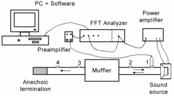
For this research, an experimental test rig was designed in order to measure the Transmission Loss of a set of muffler configurations in stationary medium. The experimental set up is based in a combination of the decomposition method originally proposed by Seybert and Ross (1977), further modifications proposed by Chung and Blaser (1980), and the transfer function correction described by Chu (1986). Figure 4 shows the experimental set up.
Figure 4. Experimental set up.
The method makes use of one moving microphone which can be flush wall mounted at fixed positions in the exhaust and the inlet of the muffler under test. The excitation consists of a random signal containing all frequencies of interest. The random noise generator of a two-channel Fourier analyzer gives the required signal. This signal is fed to a loudspeaker, which creates an acoustic pressure field in the tube. A preamplifier amplifies the signal picked up by the microphone before it is fed to the computer-controlled Fourier analyzer. The assessed data are the power spectral densities and transfer functions of signals measured at different microphone locations. Making use of these measured data, the incident and transmitted sound power can be estimated and the Transmission Loss is calculated as (Crocker, 1994)
2 1
33 11
34 12
log 10 log
10 )
exp( ) exp( log 20
S S G
G H
jks H jks
TL + +
− −
= , (17)
where s is the distance between two microphone positions (see Fig. 4), H12 is the complex transfer function between points 1 and 2, H34
is the complex transfer function between points 3 and 4, G11 is the
complex power spectral density measured at point 1, and G33 is the
complex power spectral density measured at point 3. S1 and S2 carry
the same connotations as in Eq. (16).
The complex transfer function H12 can be estimated according to
Chu (1986) as the product
2 1 12 H FHF
H = , (18)
where H1F is the complex transfer function between the signal from
the microphone placed at position 1 and the source signal, and HF2 is
the complex transfer function between the source signal and the microphone placed at position 2. Of course, H34 can be estimated in
a similar way.
Limitations and Validity of Measurements
The frequency range in which the measurements of Transmission Loss are valid is mainly given by two factors:
1) The distance between two microphone positions. In order to avoid errors associated with this factor the transfer function method is best employed in the frequency band given by (see Gerges and
Arenas, 2004; Chung and Blaser, 1980, and Abom and Bodén, 1988)
s c f s
c/2 0.8 /2 1
.
0 < < . (19)
2) The cut-off frequency of each muffler chamber.
In practical applications it is common to find tubes having circular and elliptical cross sectional areas. The first cut-off frequency of a circular cross sectional tube is given by
d c
fc=1.84 /π , (20)
where d is the tube diameter (m).
A simplified formula for the first cut-off of an elliptical tube has been given by Tsuyoshi (2001) as
a c
fc =β /2π , (21)
where the factor β is calculated in terms of the tube eccentricity, e, according to Table 1. The eccentricity of an ellipse is defined as
(
2 2)
1/2/ 1 b a
e= − , (22)
where a is half the length of the largest axis (m) and b is half the length of the smallest axis (m). Equation (21) gives results being quite similar to those obtained by means of more complex approaches involving Mathieu functions (Denia et al., 2001).
Table 1. Relationship between the eccentricity and β in Eq. (21).
Eccentricity e Factor β
0.10320 3.0624 0.20490 3.0858 0.30050 3.1208 0.39932 3.1677 0.50032 3.2228 0.60057 3.2798 0.69953 3.3342 0.79911 3.3857 0.89999 3.4358 0.90157 3.4366
For practical reasons the distance between the sound source and the muffler and the distance between the muffler and the termination should be small. A distance of five to 10 times the diameter of the tube is recommended (Abom and Bodén, 1988). In addition, the measurement point 1 (see Fig. 4), should be positioned as close as possible to the muffler, although a minimum distance of about 10 mm should be considered in order to avoid the influence of nearby fields.
A distance s=50 mm was used for the experiments. Therefore, all the results of measurements presented in the following sections can be considered as valid for frequencies above 343 Hz.
Results
outlet, and a complex muffler with several elements. For each one, the theoretical results using the Transfer Matrix Method were numerically evaluated by means of a digital computer. Since the experiments were conducted in a stationary medium and the fact that, most of the time, the transfer matrices are defined in the literature with respect to convective variables, the corresponding transfer matrices for stationary medium were obtained by means of the transformation matrix procedure described by Eqs. (13) and (14).
The results obtained experimentally and predicted by the TMM modeling of each muffler configuration are presented in this section.
Expansion Chambers
Figure 5 shows the geometry of a simple elliptic expansion chamber and the comparison between the experimental values of TL and the numerical results of TL obtained from TMM modeling. The units for the dimensions of the chamber shown in Fig. 5 and for all subsequent figures are given in mm, unless otherwise is stated. A good agreement, in general, is shown. Differences of up to 3 dB were obtained at the first and last TL loops. These are located close to the limits of the valid frequency range, determined by the microphone distance limitation given by Eq. (19) and the cut-off frequency of the chamber given by Eq. (21), where some errors are expected. Therefore, for this particular chamber the measurements are valid for frequencies above 343 Hz and below 2100 Hz.
Figure 5. Transmission loss of a simple expansion chamber using an extended tube length of 0.1 mm; TMM results (dashed line) and experimental results (solid line).
Figure 6 shows comparisons for the same chamber, but modeled as sudden expansion and sudden contraction tubes. In this latter case, the agreement between the numerical and experimental results are closer, especially at the last TL loop but less accurate at the first TL loop. Figures 5 and 6 show clearly the errors in predicting TL above the cut-off frequency. The comparisons show that the expansion chamber is more accurately modeled as sudden expansion
and sudden contraction tubes. The maximum and minimum TL are located at frequencies fmax and fmin, respectively. According to Wu
(1970) these frequencies can be predicted as
L c n
fmax =(2 +1) /4 , (23)
and
L nc
fmin =2 /4 , (24)
where L is the length of the simple expansion chamber (m) and n is an integer number.
Figure 6. Transmission loss of a simple expansion chamber modeled as sudden expansion and sudden contraction; TMM results (dashed line) and experimental results (solid line).
Chambers with Extended Tubes
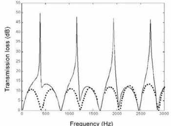
Figure 7 shows the geometry and the results from experiments and from TMM numerical predictions of an elliptical chamber with an extended tube at the inlet. Figure 8 shows the results of TL for the same chamber but with the extended tube at the outlet. An excellent agreement is observed in both cases. The agreement between TMM results and experiments is much better than in the case of a simple elliptical expansion chamber.
In addition, Fig. 9 shows the numerical results of TL obtained by means of TMM modeling for the simple expansion chamber with and without the extended tube at the inlet for comparison. It is observed that the effect of extending the entrance tube is to increase the TL peaks and to widen the frequency bands of attenuation. The numerical results shown in Fig. 9 agreed quite well with the results presented by Bento Coelho (1983) using finite elements. Here, the first characteristic peak of the TL curve is related to the resonance frequency fr, which occurs at a quarter wavelength of the extended
tube, and can be calculated as
[
4( 0.315 )]
/ L d
c
fr = + , (25)
where L is the total length of the extended tube (m) and d is its internal diameter (m). The factor 0.315 corresponds to an end correction (Pierce, 1981). Therefore, for this particular muffler geometry, the first TL peak occurs at fr=388 Hz. Additional peaks
Reflective Systems
Reflective systems are non straight-through mufflers. They can have extended tubes at the inlet, extended tubes at the outlet or both. Figures 10, 11 and 12 show the geometry and the results of TL obtained from TMM and measurements for three reflective systems.
Figure 7. Transmission loss of an expansion chamber with extended tube at the inlet; TMM results (dashed line) and experimental results (solid line).
Figure 8. Transmission loss of a simple expansion chamber with extended tube at the outlet; TMM results (dashed line) and experimental results (solid line).
In this case, good agreement between TMM and experimental results is observed for frequencies up to 1200 Hz. It can be observed that for high frequencies, the results of TL for the reflective system
with extended tube at the inlet show a similar behavior than the reflective system with extended tube at the outlet. According to Kimura (1995), the first TL peak can be calculated as
[
4( 0.315 )]
/ l d
c
fr = − , (26)
where l is the distance between the ends of the tube and the reflection wall (m) and d is the internal diameter of the extended tube (m). Therefore, for this case, the first TL peak is located at fr=820 Hz, which agrees quite well with the experimental result.
Figure 9. Comparison between TMM numerical results of transmission loss of a simple expansion chamber (dotted line) and a chamber with extended tube at the inlet (solid line).
Figure 11. Transmission loss of a reflective muffler with extended tube at the outlet; TMM results (dashed line) and experimental results (solid line).
Figure 12. Transmission loss of a reflective muffler with extended tube at both the inlet and outlet; TMM results (dashed line) and experimental results (solid line).
Silencers with Perforated Tubes
Figure 13 shows the geometry and comparison between the experimental and TMM modeling numerical results of TL for a high porosity perforated concentric tube inside an elliptic expansion chamber. A reasonable similarity in the transmission loss curves can be verified. Although some divergences are encountered, the basic behavior of the system remains the same. The general behavior of this system is similar to that of a simple expansion chamber of the same length, due to the acoustical transparency of the perforate
(given by its high porosity), as shown in Fig. 14. It is observed that the maximum TL for the concentric resonator is located at a lower frequency than for a simple expansion chamber of the same length.
Figure 13. Transmission loss of a concentric perforate tube; TMM results (dashed line) and experimental results (solid line).
Figure 14. Experimental results of TL of a concentric perforated resonator (dashed line) and an expansion chamber of the same length (solid line).
Figure 15. Transmission loss of a chamber with perforated tube at the inlet; TMM results (dashed line) and experimental results (solid line).
Figure 16. Transmission loss of a concentric perforated plugged tube; TMM results (dashed line) and experimental results (solid line).
It can be seen that the agreement between the numerical and experimental results shown in Fig. 16 is not as good as the results
presented in Fig. 15. Since a concentric perforated plugged tube represents a combination of a cross-flow expansion element and a cross-flow contraction element, it is necessary to evaluate twice the normalized partition impedance of the perforate. As mentioned before, this impedance has not been obtained theoretically and empirical expressions were used in calculating the corresponding transfer matrices. In addition, for this particular geometry, the influence of viscous effects could be more important. This could lead to some numerical errors that can explain the differences between the results presented in Figs. 15 and 16.
Real Muffler
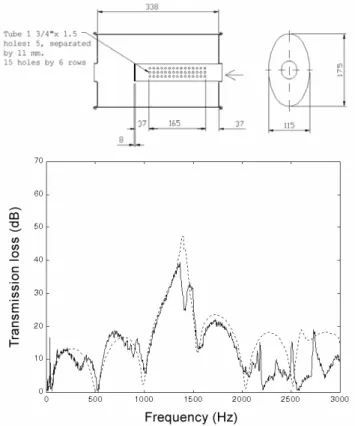
A more complex geometry, as found in real mufflers, was finally considered for modeling using TMM and experimental testing. The results presented in Fig. 17 show a good agreement between theoretical predictions and the experimental measurements.
It is observed that this complex muffler presents three significant TL peaks below 2 kHz. The TMM modeling results predicted quite reasonably the first two of them. In addition, a good prediction of the drop in TL around 1100 Hz is also observed.
Figure 17. Transmission loss of a real muffler having a complex geometry; TMM results (dashed line) and experimental results (solid line).
Conclusions
that a simple expansion chamber can be accurately modeled as a sudden expansion and sudden contraction. The TMM results predicted that the effects of extending the entrance tube in a simple expansion chamber are to increase the TL peaks and to widen the frequency bands of attenuation. The results predicted by TMM modeling agreed quite well with those presented by Bento Coelho (1983) and Kimura (1995) using more complex approaches.
When using the TMM to model a concentric perforated plugged tube the results were not as good as the results obtained when using one perforated tube. This could be due to the empirical expressions used in the calculation of the corresponding transfer matrices, which would require additional experimental studies, and the fact that the viscous effects could be of importance in this case.
Finally, for a reasonable complex geometry and not considering dissipative systems, it can be concluded that it is possible to use the TMM for predicting the acoustic behavior of mufflers in the low frequency range. Therefore, the method can be used to design a prototype muffler that would reduce the noise produced at the firing engine frequency and its first few harmonics, where the effects of higher order modes can be neglected. Since this method can be easily implemented in a digital computer, it can be used with confidence as a design guide and optimization of exhaust systems.
However, since the prototype design using the TMM would be based on the predicted Transmission Loss, to bypass the influence of the source impedance and the termination end, it is clear that differences between predicted TL and measured Insertion Loss will be observed in practice. Therefore, the final evaluation of the muffler will require field tests based on the measured Insertion Loss.
Further work has to be done to include the effects of a mean flow in the experimental set up and, additionally, the inclusion of higher order modes in the transfer matrices, which should increase the frequency range in which the predicted values would be reliable.
Acknowledgments
The authors acknowledge the support given by the Brazilian National Council for Scientific Research, Development, and Technology (CNPq), the Portuguese (ICCTI), and the Chilean CONICYT-FONDECYT under grant No 7020196.
References
Abom, M. and Bodén, H., 1988, Error Analysis of Two-Microphone Measurements in Ducts with Flow, Journal of the Acoustical Society of America, Vol. 83, No. 6, pp. 2429-2438.
Alfredson, R.J., 1970, The Design and Optimization of Exhaust Silencers, Ph.D. thesis, University of Southampton, UK.
Chu, W.T., 1986, Transfer Function Technique for Impedance and Absorption Measurements in an Impedance Tube using a Single Microphone, Journal of the Acoustical Society of America, Vol. 80, No. 2, pp. 555-560.
Chung, J.Y. and Blaser, D.A., 1980, Transfer Function Method of Measuring In-Duct Acoustic Properties: I. Theory and II. Experiment, Journal of the Acoustical Society of America, Vol. 68, No. 3, pp. 907-921.
Craggs, A., 1989, the Application of the Transfer Matrix and Matrix Condensation Methods with Finite Elements to Duct Acoustics, Sound and Vibration, Vol. 132, pp. 393-402.
Bento Coelho, J.L., 1983, Acoustic Characteristics of Perforate Liners in Expansion Chambers, Ph.D. thesis, University of Southampton, UK.
Crocker, M.J., 1994, The Acoustical Design and Testing of Mufflers for Vehicle Exhaust Systems. Proceedings of the 1st Congress Brasil/Argentine and 15th SOBRAC Meeting, Florianópolis, Brazil, pp. 47-96.
Davies, P.O.A.L., 1964, The Design of Silencers for Internal Combustion Engine, Journal of Sound and Vibration, Vol. 1, No. 2, pp. 185-201.
Davies, P.O.A.L., 1993, Realistic Models for Predicting Sound Propagation in Flow Duct Systems, Noise Control Engineering Journal, Vol. 40, pp. 135-141.
Davis, D.D., Stokes, G.M., Moore, D. and Stevens, G.L., 1954, Theoretical and Experimental Investigation of Mufflers with Comments on Engine Exhaust Muffler Design, NACA Report 1192.
Denia, F.D., Albelda, J., Fuenmayor, F.J. and Torregrosa, A.J., 2001, Acoustic Behavior of Elliptical Chamber Mufflers, Journal of Sound and Vibration, Vol. 241, No. 3, pp. 401-421.
Dowling, J.F. and Peat, K.S., 2004, An Algorithm for the Efficient Acoustic Analysis of Silencers of Any General Geometry, Applied Acoustics, Vol. 65, pp. 211-227.
Félix, S. and Pagneaux, V., 2002, Multimodal Analysis of Acoustic Propagation in Three-Dimensional Bends, Wave Motion, Vol. 36, No. 1, pp. 157-168.
Gerges, S.N.Y. and Arenas, J.P., 2004, Fundamentals of Noise and Vibration Control (in Spanish), NR Editora, Florianópolis, 765 p.
Igarashi, J. and Toyama, M., 1958, Fundamentals of Acoustic Silencers, Report No. 339, Aeronautical Research Institute, University of Tokyo, pp. 223-241.
Jayaraman, K. and Yam, K., 1981, Decoupling Approach to Modeling Perforated Tube Muffler Components, Journal of the Acoustical Society of America, Vol. 69, No. 2, pp. 390-396.
Kim, J.T. and Ih, J.G., 1999, Transfer Matrix of Curved Duct Bends and Sound Attenuation in Curved Expansion Chambers, Applied Acoustics, Vol. 56, pp. 297-309.
Kimura, M.R.M., 1995, Measurement and Acoustic Simulation of Vehicle Mufflers (in Portuguese), M.Sc. Thesis, Universidade Federal de Santa Catarina, Brazil.
Mechel, F.P., 2002, Formulas of Acoustics, Springer-Verlag, Berlin, 1175 p.
Munjal, M.L., 1975, Velocity Ratio-Cum-Transfer Matrix Method for the Evaluation of a Muffler with Mean Flow, Journal of Sound and Vibration, Vol. 39, No. 1, pp. 105-119.
Munjal, M.L., 1987, Acoustics of Ducts and Mufflers. 1st Ed., John Wiley and Sons, New York, 328 p.
Munjal, M.L., 1997, Plane Wave Analysis of Side Inlet/Outlet Chamber Mufflers with Mean Flow, Applied Acoustics, Vol. 52, pp. 165-175.
Munjal, M. L., Rao K.N. and Sahasrabudhe, A.D., 1987, Aeroacoustic Analysis of Perforated Muffler Components, Journal of Sound and Vibration, Vol. 114, No. 2, pp. 173-188.
Peat, K.S., 1988, A Numerical Decoupling Analysis of Perforated Pipe Silencer Elements, Journal of Sound and Vibration, Vol. 123, No. 2, pp. 199-212.
Pierce, A.D., 1981, Acoustics: An Introduction to its Physical Principles and Applications, Mc Graw – Hill Series in Mechanical Engineering, p. 337-357.
Rao, K.N. and Munjal, M.L., 1986, Experimental Evaluation of Impedance of Perforates with Grazing Flow, Journal of Sound and Vibration, Vol. 108, No. 2, pp. 283-295.
Sathyanarayana, Y. and Munjal, M.L., 2000, A Hybrid Approach for Aeroacoustics Analysis of the Engine Exhaust System, Applied Acoustics, Vol. 60, pp. 425-450.
Seybert, A.F. and Ross, D.F., 1977, Experimental Determination of Acoustic Properties Using a Two-Microphone Random-Excitation Technique, Journal of the Acoustical Society of America, Vol. 61, No. 5, pp. 1362-1370.
Sullivan, J.W., 1979, A Method of Modeling Perforated Tube Muffler Components, Journal of the Acoustical Society of America, Vol. 66, No. 3, pp. 772-788.
Sullivan, J.W. and Crocker, M.J., 1978, Analysis of Concentric-Tube Resonators having Unpartitioned Cavities, Journal of the Acoustical Society of America, Vol. 64, No. 1, pp. 207-215.
Thawani, P.T. and Noreen, R.A., 1988, Computer-Aided Analysis of Exhaust Mufflers, The American Society of Mechanical Enginners, New York, p. 1-7.
Tsuyoshi, N., 2001, Private Communication, Kumamoto Inst. of Technology, Japan.