Estratégias com garantia de estabilidade para a integração de controle preditivo...

Strategies with guarantee of stability for the integration of Model

Predictive Control and Real Time Optimization

Tese apresentada à Escola Politécnica de São Paulo da Universidade de São Paulo para obtenção do Título de Doutor em Engenharia.

Strategies with guarantee of stability for the integration of Model

Predictive Control and Real Time Optimization

Tese apresentada à Escola Politécnica de São Paulo da Universidade de São Paulo para obtenção do Título de Doutor em Engenharia.

Área de concentração: Engenharia Química

Orientador: Prof. Dr. Darci Odloak

Este exemplar foi revisado e alterado em relação à versão original, sob responsabilidade única do autor e com a anuência de seu orientador. São Paulo, 11 de abril de 2012.

Assinatura do autor ____________________________

Assinatura do orientador _______________________

FICHA CATALOGRÁFICA

FICHA CATALOGRÁFICA

Alvarez Toro, Luz Adriana

Strategies with guarantee of stability for the integration of model predictive control and real time optimization / L.A. Alvarez Toro. -- ed.rev. -- São Paulo, 2012.

173 p.

Tese (Doutorado) - Escola Politécnica da Universidade de São Paulo. Departamento de Engenharia Química.

ACKNOWLEDGEMENTS (In Portuguese)

Ao Professor Darci Odloak pela competência com que orientou e acompanhou esta Tese. Para ter me dado a oportunidade de trabalhar em Controle Preditivo e de fazer uma pesquisa enriquecedora.

Aos membros da Banca Examinadora: os Professores Luis Claudio Oliveira, Claudio Garcia, Oscar Sotomayor e Dr. Antonio Carlos Zanin, pela leitura, correção e sugestões de melhora desta Tese.

Aos Professores Galo Le Roux e Roberto Guardani do LSCP e ao Dr. Lincoln Moro da Petrobrás pelas críticas e comentários sobre uma primeira versão deste trabalho.

Ao Professor Oscar A. Z. Sotomayor pelas discussões e pela sua colaboração nos primeiros meses quando recém cheguei no Brasil.

Ao Professor Reinaldo Giudici pela resposta a algumas dúvidas na parte de polimerização. Aos Professores Hernán Alvarez e Jairo Espinosa da Universidad Nacional de Colombia por terem me motivado a continuar pesquisando em controle.

À Professora Cristina Borba da EP-USP por todas as ferramentas fornecidas no curso de redação acadêmica em inglês, foram muito úteis para escrever esta Tese.

Aos companheiros e o pessoal do LSCP e do Departamento de Engenharia Química. À minha familia na Colômbia e meu noivo Christophe.

ABSTRACT

RESUMO

NOMENCLATURE

0ny Matrix with entries equal to zero and dimension ny

A State matrix of the state-space model in discrete time B Input matrix of the state-space model in discrete time C Output matrix of the state-space model in discrete time

Cu Weight of the deviation of the input targets in the objective function of the Target

Calculation layer (Chapter 3)

Cy Weight of the deviation of the output targets in the objective function of the

Target Calculation layer (Chapter 3)

C_ε Weight of the slack variable in the objective function of the Target Calculation

layer (Chapter 3)

d Measured disturbance (Chapter 1)/ gradient vector of the economic function or

convex function (Chapter 4)

0

D Static gain matrix defined in the OPOM model for the states xs, see Appendix B

0

Dɶ Matrix constructed from D0 appearing in the terminal state constraint of the

infinite horizon MPC

0

i

D Static gain matrix of the model i

0

n

D Static gain matrix of the nominal model

0

t

D Static gain matrix of the true model

d

D Matrix defined in the OPOM model for the states xd, see Appendix B

d i

D Matrix Dd of the OPOM model (Appendix B) for the model i

d n

d t

D Matrix Dd of the OPOM model (Appendix B) for the true model

i

D Matrix defined in the OPOM model for the states xi, see Appendix B 1

i m

D Matrix constructed from Di appearing in the terminal constraint for the integrating

state xi of the infinite horizon MPC for integrating systems (Chapter 2)

2im

D Matrix constructed from Di appearing in the terminal state constraint of the

infinite horizon MPC for integrating systems (Chapter 2)

D0 Zero-th order moment of the dead-polymer D1 First order moment of the dead-polymer D2 Second order moment of the dead-polymer

0

f Hypothetic fixed value for the economic function feco Economic function

fi Initiator efficiency in the styrene polymerization process

F Matrix defined for the OPOM model, see Appendix B Fe Economic function or convex function

Fi Matrix F of the OPOM model (Appendix B) for the model i

Fn Matrix F of the OPOM model (Appendix B) for the nominal model

Ft Matrix F of the OPOM model (Appendix B) for the true model

G Hessian matrix in the gradient calculation of the economic function or convex

function ( )s

G Transfer function matrix

hA Overall heat transfer coefficient of the styrene reactor

I Initiator specie of the styrene polymerization process

Iɶ Matrix constructed from Inu appearing in the input target constraint of MPC

[I] Concentration of specie I in the styrene reactor

[If] Concentration of specie I in the feed of the styrene reactor

nu

I Identity matrix with dimension nu

ny

*

ny

I Matrix defined in the OPOM model for integrating systems, see Appendix B ki Rate constant for initiation reaction in the styrene polymerization process

kd Rate constant for initiator decomposition in the styrene polymerization process

kp Rate constant for propagation reaction in the styrene polymerization process

kt Rate constant for termination reaction in the styrene polymerization process

Kui Parameter of the convex function of the targets for the input i

Kyi Parameter of the convex function of the targets for the output i

L Number of models that define the uncertainty m Control horizon of the MPC

M Monomer specie in the styrene reactor in the styrene polymerization process [M] Concentration of specie M in the styrene reactor

[Mf] Concentration of specie M in the feed of the styrene reactor

m

M Molecular weight of the monomer specie

n

M Number-average molecular weight of the polymer

w

M Weight-average molecular weight of the polymer na Number of poles of the linear system

nd Total number of stable poles in the multivariable system, it is the product nu.ny.na nu Number of inputs

nut Number of targets for the inputs

ny Number of outputs

nyt Number of targets for the outputs

N Matrix defined for the OPOM model, see Appendix B P Weight of the gradient of the convex function, see Chapter 4

[P] Total concentration of live-polymers in the styrene reactor

Pn Live-polymer chain with size n in the styrene polymerization process PD Polydispersity of the polymer

Qc Flow rate of cooling jacket fluid in the styrene reactor

Qi Initiator flow rate in the styrene reactor

i

Q Nominal value for the initiator flow rate in the styrene reactor Qm Monomer flow rate in the styrene reactor

m

Q Nominal value for the monomer flow rate in the styrene reactor Qs Solvent flow rate in the styrene reactor

Qt Total flow rate in the styrene reactor

Qu Weight of the input target in the objective function of MPC

Qy Weight of the output prediction error in the objective function of MPC

R Radical specie of the styrene polymerization process

R Weight that penalizes the input changes in the objective function of MPC S Weight of the slack variable in the objective function of MPC

Si Weight of the slack for the integrating state in the objective function of MPC

Su Weight of the input slack in the objective function of MPC

Sy Weight of the output slack in the objective function of MPC

T Temperature of the styrene reactor

Tc Temperature of the cooling jacket fluid in the styrene reactor

Tcf Temperature of the cooling jacket fluid in the feed of the styrene reactor

Tf Temperature of styrene reactor feed

Tn Dead-polymer chain with size n in the styrene polymerization process u Input of the process system

u0 Initial value of the input

udes Input targets calculated by the Target Calculation layer

i

u Nominal value of the input i umax Maximum bound for the input umin Minimum bound for the input

uRTO Input targets calculated by the RTO layer

uS,min Minimum value of the input for scaling uscaled Scaled value of the input

U Feasible set of the inputs V Volume of the styrene reactor

c

V Volume of the cooling jacket of the styrene reactor Vk Objective function at time step k

x State of the process system

xi Integrating component of the state of the OPOM model, see Appendix B xd Stable component of the state of the OPOM model, see Appendix B

xs Integrated state component produced by the incremental form of the OPOM

model, see Appendix B

0

s

x Initial value of the state xs y Output of the process system

ˆ( )

y ∞ Stationary prediction of the output

ˆ ( )∞

y Vector of stationary prediction of the outputs

y0 Initial value of the output

ydes Output targets calculated by the Target Calculation layer

ymax Maximum bound for the output ymin Minimum bound for the output

yRTO Output targets calculated by the RTO layer

yS,max Maximum value of the output for scaling yS,min Minimum value of the output for scaling yscaled Scaled value of the output

ysp Set-point for the output

Greek letters

δ Slack variable of the infinite horizon MPC i

s

δ Slack variable for the outputs in the infinite horizon MPC

u

δ Slack variable for the inputs

y

δ Slack variable for the outputs in the infinite horizon MPC

r

H

∆ Heat of polymerization

t

∆ Sample time ( )

u k

∆ Single input move at time step k

k

u

∆ Vector of input moves from time step k to m−1 u

∆ Total move of the input vector from time step k−1 to k+ −m 1

max

u

∆ Maximum move of the manipulated input ε Slack variable of the Target Calculation layer η Intrinsic viscosity of the polymer

θ Set of matrices of the OPOM model for which the uncertainty is defined

t

θ Set of matrices with uncertainty of the OPOM model for the true model

n

θ Set of matrices with uncertainty of the OPOM model for the nominal model

i

θ Set of matrices with uncertainty of the OPOM model of the model i

p

C

ρ Mean heat capacity of styrene reactor fluid

cCpc

ρ Heat capacity of cooling jacket fluid of the styrene reactor

u u

ς +∆ Second order approximation of the gradient

CONTENTS

Page

CHAPTER 1. INTRODUCTION……….1

1.1 Real Time Optimization and Model Predictive Control………...1

1.2 Stability of MPC controllers……….4

1.3 Zone Control……….6

1.4 Outline of the Thesis………...8

1.5 Publications………...8

CHAPTER 2. STABLE MODEL PREDICTIVE CONTROL WITH INPUT TARGETS FOR INTEGRATING SYSTEMS……….10

2.1 Introduction………10

2.2 Prediction model for the integrating system………11

2.3 Stable MPC with input targets in one step………..12

Theorem 2-1………15

2.4 Stable MPC with input targets in two steps………24

Theorem 2-2………..26

2.5 Example: The desiobutanizer distillation column………...28

2.6 Conclusions……….36

CHAPTER 3. ROBUST INTEGRATION OF MODEL PREDICTIVE CONTROL AND REAL TIME OPTIMIZATION………..38

3.1 Introduction………38

3.2 Structure of the prediction model………...39

3.3 Stable RTO/MPC………..40

Theorem 3-1………..43

3.4 Robust RTO/MPC……….46

3.5 Example. Linear system………..51

3.5.1 Simulation of Stable RTO/MPC………...51

3.5.2 Simulation of Robust RTO/MPC……….58

3.6 Example. Nonlinear system………61

Process description………61

Control system………...65

3.6.1 Simulation of Stable RTO/MPC………...67

3.6.2 Simulation of Robust RTO/MPC……….71

3.6.3 Comparison to a typical MPC controller………..75

Case A………76

Case B………80

3.6.4 Complete RTO with the robust structure………..83

3.7 Conclusions……….89

CHAPTER 4. STABLE MODEL PREDICTIVE CONTROL WITH GRADIENT OF A CONVEX FUNCTION OF THE TARGETS……….91

4.1 Introduction……….91

4.2 MPC with infinite horizon and input targets………...92

4.3 Integration of RTO and MPC through the economic gradient………....95

4.3.1 Gradient of the economic function………...95

4.3.2 Model predictive control with real time optimization………..96

4.4 Stable MPC with gradient of a convex function……….97

Theorem 4-1………100

Remark 1……….109

Remark 2……….111

4.5 Example: Linear system………111

4.6 Example: Polymerization reactor………..116

4.6.1 Control system………116

4.6.2 Simulation results………...117

4.7 Extension to uncertain systems: Robust MPC………..124

4.8 Example: System with polytopic uncertainty………...129 4.9 Conclusions………...134

CHAPTER 5. CONCLUSIONS AND DIRECTIONS FOR FUTURE WORK…………135

REFERENCES………139

APPENDIX A: Derivation of the model equations for the styrene reactor ……..……….144

LIST OF FIGURES

Page

CHAPTER 1

Figure 1.1. Integration of MPC and RTO in a two-layer structure……….2

Figure 1.2. Integration of MPC and RTO in a three-layer structure………...3

Figure 1.3. Integration of MPC and RTO in an one-layer structure………...4

Figure 1.4. Process Output controlled by zones……….7

CHAPTER 2 Figure 2.1. Schematic diagram of the deisobutanizer column……….29

Figure 2.2. Inputs Targets (− − −) and inputs of the deisobutanizer column with Controller I (− · − ·−) and Controller II (——)………33

Figure 2.3. Outputs of the deisobutanizer column with Controller I (− _· − _·−) and Controller II (——)………...34

Figure 2.4. Objective functions of Controller I (− _· − _·−) and Controller II (——) for the deisobutanizer column……….35

Figure 2.5 Slack variable for the integrating output of the deisobutanizer column with Controller I (− _· − _·−) and Controller II (——)……….36

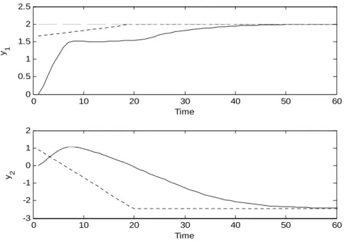
CHAPTER 3 Figure 3.1. System outputs () and computed targets ydes(⋅⋅⋅⋅⋅⋅) for reachable optimizing target (  )……….53

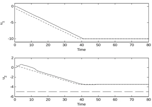
Figure 3.2. System inputs () and computed targets udes(⋅⋅⋅⋅⋅⋅) for reachable optimizing target (  )………...53

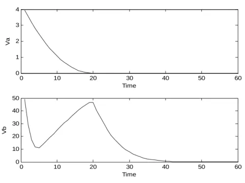
Figure 3.3. Objective function of problems P3-1a and P3-1b for reachable optimizing target………...54

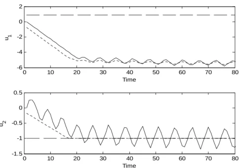
Figure 3.5. System inputs () and computed targets udes(⋅⋅⋅⋅⋅⋅) for unreachable

optimizing target (  )……….55 Figure 3.6. Objective function of problems P3-1a and P3-1b for unreachable optimizing

target………...56 Figure 3.7. System outputs () and computed targets ydes(⋅⋅⋅⋅⋅⋅) with model

mismatch………57 Figure 3.8. System inputs () and computed targets udes(⋅⋅⋅⋅⋅⋅) with model

mismatch………57 Figure 3.9. Uncertain system: outputs (), computed output targets ydesfor model 1

(⋅⋅) and model 2 (⋅⋅⋅⋅⋅⋅) and optimizing output target (  )………59 Figure 3.10. Uncertain system: inputs (), computed targets udes(⋅⋅⋅⋅⋅⋅) and

optimizing input target (  )………...60 Figure 3.11. Uncertain system objective function of problems P3-2a and P3-2b, model 1

() and model 2 (  )………....60 Figure 3.12. Process diagram of the styrene polymerization reactor………...62 Figure 3.13. Stable RTO/MPC simulation. Outputs (black solid line), calculated output targets (blue dashed line), RTO output target (green dashed line) and output zone (red dashed line)………69 Figure 3.14. Stable RTO/MPC simulation. Inputs (black solid lines), calculated input targets (blue dashed lines), RTO input target (green dashed line)………70 Figure 3.15. Stable RTO/MPC simulation. Objective functions of P3-1a and P3-1b…….70

Figure 3.16. Output values T and η for the steady states where each linear model MN,

M1, M2 and M3 where obtained………...72 Figure 3.17. Robust RTO/MPC simulation. Outputs (black solid lines), calculated

output targets (blue dashed lines), RTO output target (green dashed line) and output zone (red dashed lines)………..74 Figure 3.18. Robust RTO/MPC simulation. Inputs (black solid lines), calculated input targets (blue dashed lines), RTO input target (green dashed line)………74 Figure 3.19. Robust RTO/MPC simulation. Objective functions of P3-2a and P3-2b...75

Output bounds. Blue dashed line: calculated targets. Green dashed line: RTO targets. Solid line: Process outputs………78 Figure 3.21. Process inputs with the robust structure in Case A. Blue dashed line:

calculated input targets. Green dashed line: RTO input targets. Solid line: Process inputs……….78 Figure 3.22. Process outputs for conventional MPC controller in the Case A. Red

dashed line: Output bounds. Blue dashed line: RTO targets. Solid line: Process outputs………..79 Figure 3.23. Process inputs for conventional MPC in Case A. Blue dashed line: RTO input targets. Solid line: Process inputs………79 Figure 3.24. Outputs with robust structure in Case B. Red dashed line: Output bounds. Blue dashed line: calculated targets. Green dashed line: RTO targets. Solid line: Process outputs………..81 Figure 3.25. Process inputs with robust structure in Case B. Blue dashed line: calculated input targets. Green dashed line: RTO input targets. Solid line: Process inputs………...81 Figure 3.26. Process outputs for conventional MPC in Case B. Red dashed line: Output bounds. Blue dashed line: RTO targets. Continuous line: Process outputs………...82 Figure 3.27. Process inputs for conventional MPC in Case B. Blue dashed line: RTO

input targets. Solid line: Process inputs……….82 Figure 3.28. Process outputs with the RTO operating in presence of disturbances. Red

dashed line: Output bounds. Blue dashed line: calculated targets. Green dashed line: RTO targets. Solid line: Process outputs………...87 Figure 3.29. Process inputs with RTO operating in presence of disturbances. Blue

dashed line: calculated input targets. Green dashed line: RTO input targets. Solid line: Process inputs………....87 Figure 3.30. Objective functions of the robust algorithm with the RTO operating in

presence of disturbances………....88 Figure 3.31. Production rate of the process with the RTO operating in presence of

disturbances………88 Figure 3.32. Polydispersity of the produced polymer with the RTO operating in presence

CHAPTER 4

Figure 4.1. System outputs and zones of the linear system controlled by the stable MPC with gradient of a convex function………...113 Figure 4.2. System inputs and input targets of the linear system controlled by the stable

MPC with gradient of a convex function……….114 Figure 4.3. Gradient of the convex function when linear system is controlled by the

stable MPC with gradient………...114 Figure 4.4. Objective function of the the stable MPC with gradient of a convex

function………115 Figure 4.5. Process Outputs of the gradient controller (blue solid line) and output zone

limits (red dashed line)……….119 Figure 4.6. Process Inputs of the gradient controller………..119 Figure 4.7. Evolution of the economic function f of the process with gradient MPC……120

Figure 4.8. Evolution of the components of the gradient vector d of the economic

function………120 Figure 4.9. Process Outputs of the gradient controller (blue solid line), the target

controller (pink solid line) and output zone limits (red dashed line)………...122 Figure 4.10. Process Inputs of the gradient controller (blue solid line), the target

controller (pink solid line) and input targets (red dashed line)………123 Figure 4.11. Evolution of the economic function f of the process with gradient MPC

(blue line) and target MPC (pink line)……….123 Figure 4.12. System outputs (solid line) and outputs set-points (dashed line) for the

Robust MPC with gradient of a convex function of the targets………..131 Figure 4.13. System Inputs (solid line) and Input targets (dashed line) for the Robust MPC with gradient of a convex function of the targets………...132 Figure 4.14. Objective function of the nominal model for the Robust MPC with gradient of a convex function of the targets………...133 Figure 4.15. Components of the gradient of the convex function for the Robust MPC

LIST OF TABLES

Page

CHAPTER 3

CHAPTER 1

INTRODUCTION

Model Predictive Control (MPC) refers to a class of computer control algorithms that utilize an explicit process model to predict the future response of a plant. At each control interval an MPC algorithm attempts to optimize future plant behavior by computing a sequence of future manipulated variable adjustments. The first input in the optimal sequence is then sent to the plant, and the entire calculation is repeated at subsequent time intervals. Predictive control was originated in the late seventies and has been developed considerably over the last few years, both within the research control community and in industry. The reason for this success can be attributed to the fact that Model Predictive Control is, perhaps, the most general way of posing the process control problem in the time domain (Camacho and Bordons, 2004). It can be used to control a great variety of processes, from those with relatively simple dynamics to other more complex ones. MPC is also the most popular strategy to deal with multivariable control problems, and presents a series of advantages, for instance, process constraints can be handled naturally. Another interesting feature of the predictive control is the natural way of introducing feedforward control to compensate for measured disturbances and to combine this with the feedback, as it takes the last output measure to predict the future behavior of the plant. Originally developed to meet the specialized control needs of power plants and petroleum refineries, the MPC technology can now be found in a wide variety of application areas in the process industry.

1.1. REAL TIME OPTIMIZATION AND MODEL PREDICTIVE CONTROL

but to operate the plant such that the net return of investment is maximized in the presence of disturbances and uncertainties, exploiting the available measurements (Engell, 2007). The economic objective is actually specified through “set-points” or “targets” for some process variables. The control system has to bring those process variables to those optimal values. Thus, in practice, MPC controllers are implemented as part of a multilevel hierarchy of control functions (Ying and Joseph, 1999; Kassmann et al., 2000; Tatjewski, 2008; Darby et al., 2011), as depicted in Figure 1.1.

RTO

(Nonlinear steady-state model)

MPC

(Dynamic model)

Process System

,

RTO RTO

y u

( )

u k y k( )

Figure 1.1. Integration of MPC and RTO in a two-layer structure

presence of disturbances can shift the economic optimum from the initial point, computed by the real time optimizer. Since the RTO routine is not executed at the same frequency as the MPC controller, the process may operate at suboptimal conditions until the next updating of the RTO targets. This is the reason to insert a steady-state target optimizer between the RTO and the MPC layers, which results in the three-layer structure shown in Figure 1.2.

, , ,

des k des k

y u

RTO

(Nonlinear steady-state model)

Target Calculation

Process System

,

RTO RTO

y u

( )

u k y k( )

MPC

(Dynamic model)

( )

d k

Figure 1.2. Integration of MPC and RTO in a three-layer structure

to integrate the Dynamic Real Time Optimization (D-RTO) and MPC (Würth et al., 2009, 2011).

RTO + MPC

(Dynamic model)

Process System

( )

u k y k( )

Figure 1.3. Integration of MPC and RTO in an one-layer structure

On the other hand, some studies (Zanin et al., 2002; Biegler and Zavala, 2009; De Souza et al., 2010; Ochoa et al., 2010) have attempted to integrate the RTO layer to the MPC controller, in such a way that both the economic objective and the dynamic regulation are solved in one single optimization routine. This approach is denoted as one-layer structure and is shown in Figure 1.3. The strategies proposed in this Thesis for the integration of RTO and MPC considers the two and three-layer approaches.

1.2. STABILITY OF MPC CONTROLLERS

hand, the regulator of Rawlings and Muske does not include the case of unmeasured disturbances. The use of a model in the positional form described by eq. (1.1) can result in offset.

( 1) ( ) ( )

( ) ( )

x k Ax k Bu k

y k Cx k

+ = +

= (1.1)

To handle this, in Odloak (2004), it is suggested to use a model in the incremental form as defined in eq. (1.2).

( 1) ( ) ( )

( ) ( )

x k Ax k B u k

y k Cx k

+ = + ∆

= (1.2)

This work is based on an infinite horizon controller, which uses for prediction a model representation denoted as OPOM (Output Prediction Oriented Model). A terminal state constraint is also incorporated and to soften this constraint, slack variables are included in the MPC optimization problem. This controller has nominal stability and was also extended to uncertain systems.

unreachable steady-states, Limon et al. (2008) define an artificial steady-state for the system inputs and outputs that are considered as additional decision variables of the control problem. The endpoint constraint is written in terms of the artificial steady-state and the cost is extended with a term that penalizes the deviation between the artificial steady-state and the desired one. A similar approach is followed by Shead and Rossiter (2007) who define the reachable steady-state in terms of a vector of unknown parameters that become additional decision variables of the dual mode MPC. In Gonzalez and Odloak (2009), the controller assumes that the process system has targets for some of the inputs and outputs, and the remaining outputs are controlled by zones.

Usually, the real processes are not rigorously represented through linear models, but only an approximated representation is obtained. In that case, the stability is only guaranteed if the model used for prediction is exactly the same plant model, this is known as nominal stability. In order to improve the stability of the closed-loop, the model uncertainty should be included in the MPC controller. For several classes of uncertainty, many robust approaches have been proposed (Badgwell, 1997; Rodrigues and Odloak, 2003; Odloak, 2004) and apparently they can be applied in practice without major difficulties (Porfirio et al., 2003). In this Thesis the robust stability of the integration of MPC and RTO is adressed in Chapters 3 and 4.

1.3. ZONE CONTROL

In practice, one way to implement zone control in predictive controllers is setting to zero the term corresponding to the output prediction error in the objective function of the MPC when the controller outputs are inside the zone (Zanin et al., 2002; De Souza et al., 2010). If any output overpasses the desired zone, the contribution of the output error is activated for this output and the value of the set-point is the one corresponding to the exceeded bound, ymax or ymin.

Figure 1.4. Process Output controlled by zones

proposed in this work adopt the zone control strategy as well as the infinite prediction horizon to guarantee stability.

1.4. OUTLINE OF THE THESIS

This Thesis presents and analyzes stable MPC strategies that can be inserted in a control structure where RTO is included and sends targets to the MPC controller. In Chapter 2, an MPC controller with optimizing targets that deals with integrating systems is described and tested. Then, a three-layer RTO/MPC structure that guarantees robust stability for the intermediary layer and the MPC controller is proposed in Chapter 3. Chapter 4 presents an MPC algorithm which uses the gradient of a convex function to follow the RTO targets. Stability is proved for all the proposed controllers, which operates under zone control. The controllers described in Chapters 3 and 4 are tested for both linear and nonlinear systems. As Chapters 2, 3 and 4 present different control strategies, they can be read separately. The general conclusions are finally presented in Chapter 5.

1.5. PUBLICATIONS

Some of the results of this Thesis appear in the following journals and events:

International Journals

• Alvarez, L.A.; Francischinelli, E.; Santoro, B.; Odloak, D. (2009) Stable model

predictive control for integrating systems with optimizing targets. Industrial &. Engineering Chemistry Research, 48, pp. 9141-9150.

• Alvarez, L.A.; Odloak, D. (2010) Robust integration of Real Time Optimization

with linear Model Predictive Control. Computers & Chemical Engineering, 34, pp.

• Alvarez, L.A.; Odloak, D. (2012) Optimization and Control of a Continuous

Polymerization Reactor. Brazilian Journal of Chemical Engineering. Accepted

for publication.

International Congresses

• Alvarez, L.A.; Odloak, D. (2010) A simplified RTO/MPC algorithm with infinite

horizon for industrial process operation. 19th International Congress of Chemical and Process Engineering, CHISA 2010. Prague. 28 August - 1 September 2010. • Alvarez, L.A.; Odloak, D. (2011) Optimizing the operation of a polymerization

reactor via multimodel MPC. 11th international chemical and biological

CHAPTER 2

STABLE MODEL PREDICTIVE CONTROL WITH INPUT

TARGETS FOR INTEGRATING SYSTEMS

2.1. INTRODUCTION

This chapter is organized as follows. The prediction model for integrating systems is presented in section 2.2. The first algorithm that solves the control problem in one step is described in section 2.3. Then, the optimization problem presented in section 2.3 is decomposed in two steps. The first step is related to the integrating states and the second step is related to the stable states. The two-step algorithm is presented in section 2.4. Stability proofs for the two versions of the MPC controller are also provided. The controllers are simulated in a distillation system and results are discussed in section 2.5. Finally the conclusions of this chapter are presented.

2.2. PREDICTION MODEL OF THE INTEGRATING SYSTEM

In this section, the state-space model that represents the process system with integrating modes is described. It is a minimal order model with a particular structure that simplifies the development of a stable MPC with infinite prediction horizon and the integration of the controller with the real time optimization of the process plant. Here, it is assumed that the system has nu inputs and ny outputs. The state-space model adopted here is the

OPOM model (Output Prediction Oriented Model) and it is described as follows (Carrrapiço and Odloak, 2005):

) ( ) ( ) ( ) ( ) 1 ( k Cx k y k u B k Ax k x = ∆ + = + (2.1) where           = ) ( ) ( ) ( ) ( k x k x k x k x i d s ; * * 0 0 0 0 0 ny ny ny

I t I

A F I  _∆    =_{ }     ; 0 i d i D tD

B D FN

D  _{+ ∆}    =_{ }     (2.2) 0 ny ny

C=_I Ψ _; x ks( )∈ ny; xd( )k ∈ℂnd; x ki( )∈ ny t

∆ is the sampling time

*

ny

I is a diagonal matrix of dimension ny×ny whose entries are 1 for the integrating

When a transfer function model is available, a method to obtain matrices F, D0, Di, Dd

andΨis described in the Appendix B. Observe that in the model defined in eq. (2.1), it is assumed that the system may have integrating outputs (when _Di _≠0_{). When this happens,}

the three state components defined in eq. (2.2) can be interpreted as follows: s

x is the

state component corresponding to the integrating modes created by the incremental form of the model; d

x corresponds to the stable modes of the system and xi is the state

component corresponding to the true integrating outputs of the system. Since the model defined in eq. (2.1) is incremental in the inputs, it is offset free and there is no need to include an intermediary target calculation layer as in Figure 1.1, which is normally used to eliminate offset in the usual MPC implementation (Kassman et al., 2000; Muske and Rawlings, 1993).

2.3. STABLE MPC WITH INPUT TARGETS

The MPC considered here assumes that the outputs of the process system are controlled inside zones

(

)

(

)

also have targets

(

)

Assuming that k is the present time instant, the optimization problem that defines the

controller considered here is the following:

Problem P2-1

(

) (

)

(

) (

)

, , , , 1,

, , , , , , , , , , 0 , , 0 1 , , , , , 0 min ( / ) ( / ) ( / ) ( / ) ( / ) ( / )

k y k sp k u k i k k

u y

T

sp k y k i k y sp k y k i k

j

T

RTO u k u RTO u k

j m

T T T

T

y k y y k u k u u k i k i j

V

y k j k y j t Q y k j k y j t

u k j k u Q u k j k u

u k j k R u k j k S S S

∆ δ δ δ

∞ = ∞ = − = =

+ − − δ + ∆ δ + − − δ + ∆ δ

+ + − − δ + − − δ

+ ∆ + ∆ + + δ δ + δ δ + δ δ

∑

∑

∑

subject to:

( / )

u k j k U

∆ + ∈ (2.4)

0

, 2 ,

( ) [ ] 0

s i

sp k m k y k

x k −y + Dɶ −D ∆ − δu = (2.5)

,

( 1) _{nu k RTO u k} 0

u k− +I ∆ −u u − δ = (2.6)

1 ,

( ) 0

i i

m k i k

x k +D ∆ + δ =u (2.7)

min sp k, max

y ≤y ≤y (2.8)

where:               ≥ = + ∆ ≤ + ∆ + − ∆ ≤ ∆ ≤ + ∆ ≤ ∆ − + ∆ =

∑

[

]

k u k k u k k u k m k

u = ∆ ( / ) ∆ ( +1/ ) ∆ ( + −1/ )

∆ …

m

nu nu

I I I

 

 

=

 

 

ɶ _{⋯ ;} 0 0 0

m

D D D

 

 

=

 

 

ɶ _{⋯ ;}

1 [ ]

m

i i i i

m

D = D D ⋯ D , D₂im=0 ∆t Di ⋯ (m− ∆1) t Di

The first term of the objective function defined in eq. (2.3) is the output error with respect to the set-point that is also a variable of the control problem in the zone control strategy. To compute the output error, it is considered an infinite sum since stability is to be assured. It can be shown that the infinite term can be reduced via a terminal weight Q

In order to enlarge the region where the controller is feasible, slack variables δ_{y k,} , δ_{i k,} ,

,

u k

δ for the outputs, integrating states and inputs, respectively, are included in the control problem. These variables should be small enough to reduce the deviation of the original constraints, so they are penalized in the objective function using weights Sy, Si and Su.

Input constraints (2.4) are the typical MPC constraints. The constraints defined in eqs. (2.5) and (2.6) imply that the output and input errors should be minimized at the steady-state. Constraint (2.7) sets to zero the integrating states at the end of the control horizon m.

Constraint (2.8) defines the range where the output set-points should lie. For those outputs with optimizing targets, the controller considers y_min =y_max =y_RTO.

The tuning parameters of the controller resulting from the solution to Problem P2-1 are

the weight matrices Qy, and R and control horizon m as in the conventional MPC and may

follow the same tuning rules as in the conventional MPC. Additional tuning parameters of the proposed controller are Qu and the slack weight matrices Sy, Su and Si that are

related to the slack variables introduced in the control problem. These weights should be large enough in order to guarantee that the Hessian matrix of the control objective is strictly positive definite, otherwise the solution of the control problem may not be unique and the control objective will not have a minimum. Other considerations about the numerical values of these weights will be presented later in this Thesis.

Notice that the use of slacks in Problem P2-1 makes this problem always feasible, even

the integrating modes, to zero, then, the sequential solution of Problem P2-1 will force

the closed-loop system to converge to the desired steady-state.

Theorem 2-1. Feasibility and Convergence of the one-step MPC

For a system with stable and integrating outputs that can be stabilized at a desired steady-state, if at time k the optimal solution to Problem P2-1 results in a slack vector

corresponding to the integrating poles (δ_{i k,} ) equal to zero, then for the undisturbed system the solution of Problem P2-1 at any subsequent time step k+j is feasible

withδ_{i k, +j} =0 and it is possible to find a solution to Problem P2-1 at the subsequent time

steps that leads the system in closed loop to the desired steady-state.

Proof

Recursive feasibility

For the optimal solution to Problem P2-1 at time k, that results in a slack vector

corresponding to the integrating poles (δ_{i k,} ) equal to zero, the constraint corresponding to eq. (2.7) is feasible. Also, suppose that at time step k the optimal solution to Problem P2-1 is designated as

(

)

by

(

)

* *

1

* * * *

, 1 , , 1 , , 1 , , 1 ,

( 1/ ) ( 1/ ) 0

, , , 0

T

T T

k

y k y k sp k sp k u k u k i k i k

u u k k u k m k

y y

δ δ δ δ δ δ

+

+ + + +

 

∆ = ∆_ + ∆ + − _

= = = = =

ɶ ⋯

ɶ _ɶ ɶ ɶ (2.9)

Since this solution is inherited from the solution at the previous time step, it is clear that

( / 1)

u k j k U

∆ɶ + + ∈ and y_min ≤yɶ_{sp k, 1+} ≤y_max. Also, assuming that the input optimizing

1 , 1

( ) _{k RTO u k} 0

u k + ∆I uɶ ɶ ₊ −u − δɶ ₊ =

Then, constraint (2.6) is satisfied by the solution proposed in eq. (2.9). Analogously, it can be shown that

1 1

( 1) 0

i i

m k

x k+ +D ∆uɶ ₊ =

The above expression shows that constraint (2.7) is also satisfied by the solution proposed in (2.9). Then, it remains to verify if constraint (2.5) is satisfied by the solution defined in (2.9). At time step k+1, with the proposed solution, the left hand side of eq.

(2.5) can be written as follows

0

, 1 2 1 , 1

( 1) [ ]

s i

sp k m k y k

LHS =x k+ −yɶ ₊ + Dɶ −D ∆uɶ ₊ − δɶ ₊ (2.10)

Using the model expressions defined in eqs. (2.1), (2.2) and the relations contained in eq. (2.9), the expression of the eq. (2.10) can be written as follows

(

)

, ,

0 * * *

( ) ( ) ( / ) ( 1/ )

( 1/ ) ( 2 / ) ( 2) ( 1/ )

s i i

sp k y k

i i

LHS x k t x k D t D u k k y D u k k

D u k m k t D u k k m t D u k m k

= + ∆ + + ∆ ∆ − − δ + ∆ + +

+ ∆ + − − ∆ ∆ + − − − ∆ ∆ + −

⋯

⋯

(2.11)

Since eq. (2.7) is satisfied at time step k, it can be written that

* * *

,

( ) ( / ) ( 1/ )

i i i

i k

x k = − ∆D u k k − − ∆⋯ D u k+ −m k − δ (2.12)

Now, using the eq. (2.12) to eliminate the integrating state ( )i

0 * * * * *

, , 2 ,

( )

s i

k sp k y k m k i k

LHS=x k +Dɶ ∆ −u y − δ −D ∆ − ∆ δu t

Observe that if δ =*_{i k,} 0, the right hand side of the above equation becomes equal to the left side of eq. (2.5) at time k and consequently eq. (2.5) is also satisfied by the solution

defined in eq. (2.9). Then, the solution defined in eq. (2.9) is feasible.

Convergence of the objective function

To show the convergence of the objective function, let the objective function of Problem

P2-1 corresponding to the optimal solution at time step k be designated V1,*k and the value of the objective function at time step k+1 corresponding to

(

)

(

) (

)

(

) (

)

* * * * *

1, 1, 1 , , , ,

* * * * * *

, ,

( / ) ( / )

( / ) ( / ) ( / ) ( / )

T

k k sp k y k y sp k y k

T _T

RTO u k u RTO u k

V V y k k y Q y k k y

u k k u Q u k k u u k k R u k k

δ δ

δ δ

+

= + − − − −

+ − − − − + ∆ ∆

ɶ

As matrices Qy, Qu and R are assumed to be positive definite, if any of the last three terms

of the right hand side of the above equation is different from zero, then * 1,k 1 1,k

Vɶ ₊ <V . Thus,

the optimal objective at time k+1 will be smaller than the optimal objective at time k:

* *

1,k 1 1,k

V ₊ <V , or the optimal objective of Problem P2-1 is decreasing and the closed loop

system converges to a steady-state where

, ,

( ) _{sp y} 0

y ∞ −y _∞−δ _∞ =

,

( ) _{des u} 0

u ∞ −u −δ _∞ =

1, y, T y y, u, T u u,

V _∞ = δ _∞ S δ _∞+ δ _∞ S δ _∞ (2.13)

Observe also that at this steady-state, constraints (2.5) to (2.7) can be written as follows

, ,

( ) 0

s

sp y

x ∞ −y _∞−δ _∞ =

,

( ) _{RTO u} 0

u ∞ −u −δ _∞ = (2.14)

( ) 0 i

x ∞ = (2.15)

Observe that if V_1,∞ =0, then the system will stabilize at the desired steady-state given by ( ) _RTO

u ∞ =u and y( )∞ = ysp,∞ with ymin ≤ ysp,∞ ≤ ymax.

It can be shown that if the desired steady-state (optimizing inputs and outputs at their targets and the remaining inputs and outputs inside their bounds) is reachable and weight matrix Su is selected appropriately, then the closed loop system with the proposed

controller will not stabilize at the steady-state where δ_y,∞ ≠0 or δ_u,∞ ≠0. For this purpose, suppose that when the system reaches the above steady-state, Problem P2-1 is

solved again. Then, the resulting control move ∆u_∞ will have to satisfy the constraint

defined in eq. (2.6) that, at this time step, can be written as follows

' ,

( ) RTO u 0

u ∞ −u + ∆ −I uɶ _∞ δ _∞ = (2.16)

Now, considering eq. (2.14), the expression of eq. (2.16) can be written as follows

'

, , 0

u I u u

δ ∞ + ∆ −ɶ ∞ δ ∞ = (2.17)

To simplify the analysis, suppose also that the inputs are unconstrained. Then, ∆u_∞ can

be chosen according to

, 0

u I u

and consequently, from eq. (2.17) it results that '

, 0

u

δ ∞ = . Then, from eq. (2.16) follows that

'( ) ( ) _RTO

u ∞ = ∞ + ∆ =u I uɶ _∞ u

This means that the new control input will be exactly at the desired value. Corresponding to this input, the output will reach a new steady-state that is given by

0 2

'( ) s( ) i

m

y ∞ =x ∞ +_Dɶ −D _∆u_∞, which by assumption is inside the output control zone.

Then, the constraint defined in eq. (2.5) becomes

' 0 '

, 2 ,

( ) 0

s i

sp m y

x ∞ −y _∞+_Dɶ −D _∆ −u_∞ δ _∞ =

As the predicted output y'( )∞ is inside the control zone, y'sp,∞ can be chosen such that

' 0

, ( ) 2

s i

sp m

y _∞ =x ∞ +_Dɶ −D _∆u_∞ (2.19)

The combination of the two above equations produces '

, 0

y

δ ∞ = . Now, consider constraint (2.7) that will be also satisfied by control action ∆u_∞. When solving Problem P2-1 at the

steady-state, eq. (2.7) will be written as follows

'

1 ,

( ) 0

i i

m i

x ∞ +D ∆ +u_∞ δ _∞ = (2.20)

However, since from eq. (2.15) ( )i

x ∞ is null, and in the successive solution of Problem P2-1, it is assumed that the slack vector corresponding to the integrating modes is also

kept null, eq. (2.20) reduces to

1 0

i m

Then, the control action should be such that both eqs. (2.15) and (2.21) are satisfied. So, some care must be taken when defining, in the design stage of the controller, which inputs will receive target signals. For instance, the condition defined in eq. (2.21) could not be satisfied if all the inputs that are integrated by a given output have independent targets.

Now observe the objective defined in eq. (2.13). Using eq. (2.18), it is concluded that

1, , ,

T

T T

u u u u

V _∞ ≥δ _∞Sδ _∞ = ∆u_∞ I S I uɶ ɶ∆ _∞

At this point the control objective ' 1,

V _∞ corresponding to the proposed solution to Problem P2-1 can be determined. To simplify the analysis, it is assumed that the control horizon

(m) is equal to 2. In this case, the control objective corresponding to the proposed

solution to Problem P2-1 is given by

(

)

'

1, 1 2 3

T

V _∞ = ∆u_∞ G +G +G +R ∆u_∞

where

{

} {

}

{

} {

}

0 0 0 0

1 2 2

2 2 2 2

T

i i d i i d

m u u y m u u

T

i i i d d i i i d d

m y m

G D D D tD N D N Q D D D tD N D N

D tD tD FD D Q D tD tD FD D

ψ ψ ψ ψ         = −_ − _+_ + ∆ _ + −_ − _+_ + ∆ _ +         + + ∆_ ∆ _+ _{ } + ∆_ ∆ _+ _{ } ɶ ɶ

[

]

N = I

2

T

d d d d

G =_FD D _ Q FD_ D _

T T T

y

Q−F QF=F ψ QψF

(

) (

)

3

T

u u u

G = N −Iɶ Q N −Iɶ

Then, if

1 2 3

T u

G +G +G + <R I S Iɶ ɶ (2.22)

the proposed solution to Problem P2-1 has a control objective lower than V1,∞, that is

' 1, 1,

V _∞ <V _∞ , and the steady-state where δu,∞ ≠0 is not optimal. Thus, the successive

solution of Problem P2-1 will force the system to converge to the desired steady-state.

Condition to guarantee the convergence of the closed loop to the targets

To guarantee the convergence of the process system to the desired steady-state, the controller tuning parameters should satisfy the eq. (2.22), as shown above. Notice that G1, G2 and G3 do not depend on the weight matrix Sy corresponding to the slack of the output

steady-state. This does not mean that Sy can be any positive definite matrix. This is so

because the proposed controller should also provide nominal stability for the case in which the controller is applied in the conventional MPC scheme where there are no input targets and the outputs are controlled with fixed set-points. Problem P2-1 can be easily

adapted to this case by considering Qu=0 and Su=0, and there is no need to include

constraint (2.7).

Then, if δ_{i k,} is reduced to zero, the solution to Problem P2-1 produces a stabilizing

control law that leads the system inputs and outputs to the optimizing targets. For the case in which the controller is operating in the conventional approach (set-points for the outputs and no targets for the inputs), the successive application of this control law will lead the system to a steady-state where

1, , ,

T y y y

V _∞ =δ _∞Sδ _∞ (2.23)

,

( ) _{sp y} 0

y ∞ −y −δ _∞ = (2.24)

( ) 0 i

Now, Sy should be selected such that, at this steady-state slack δy,∞ is null. For this

purpose suppose that Problem P2-1 is solved when the system reaches the steady-state

where conditions (2.23) and (2.24) are satisfied. To simplify the analysis assume that the control horizon (m) is equal to 2 and the system input is unconstrained. In this case,

Problem P2-1 has only two constraints:

0 '

2 ,

( ) 0

s i

sp m y

x ∞ −y +_Dɶ −D _∆ −u_∞ δ _∞ = (2.26)

1 0

i m

B ∆ =u_∞ (2.27)

As the input is assumed to be unconstrained, it is possible to find ∆u_∞ such that

0

2 ,

i

m y

D D u_∞ δ _∞

 ₋ _{∆ =}

 ɶ  (2.28)

Now, substituting eq. (2.28) in eq. (2.23) it is easy to see that

0 0

1, 2 2

T

T i i

m y m

V _∞ = ∆u_{∞ }Dɶ −D _ S _Dɶ −D _∆u_∞ (2.29)

Then, following the same steps as the last case, it is possible to show that the control objective of Problem P2-1 at the steady-state defined above is reduced to the expression

(

)

'

1, 1 2

T

V _∞ = ∆u_∞ G +G +R ∆u_∞ (2.30)

From eqs. (2.29) and (2.30), it is clear that, in order to force slack δ_{y k,} to converge to zero, Sy has to satisfy the following condition

0 0

2 2 1 2

T

i i

m y m

D D S D D G G R

 ₋   ₋ _{> + +}

The expression (2.31) provides the minimum bound for Sy to guarantee stability for the

closed loop system. Now, observing the state matrix of the model defined in eq. (2.1), it is easy to see that the system cannot reach a steady-state where the state component xi is

not equal to zero. If this happens, state component xs will grow unbounded and so the

output will be unlimited. From constraint (2.7), at steady-state, follows that i( ) _, i

x ∞ =δ _∞,

then the slack of the integrating state will also be zero otherwise the output would be unbounded. Then, the controller behaves differently in terms of the tuning parameter Si

when compared to Sy or Su. As long as a positive definite Si is adopted, the convergence

of the system to the steady-state will not depend on the numerical value of Si.□

In Carrapiço and Odloak (2005), it is proposed to include the following contracting constraint in the infinite horizon MPC of integrating systems

, , , 1 , 1

T T

i k i i kS i k Si i k

δ δ ≤δɶ ₋ δɶ _{− (2.32)}

where δɶ_{i k, 1− is computed so as to satisfy the eq. (2.7) in the previous time step}

, 1 ( 1) 1 1

i i

i k− x k Dm uk− δɶ = −_ɶ − − ∆

( 1) ( ) ( 1)

i i i

x kɶ − =x k − ∆D u k−

The problem that arises when the constraint (2.32) is included into the Problem P2-1 to

force the decrease of the norm of the slack of the integrating output to zero is that this is not a linear constraint. Using the Schur complement, it can be converted in a linear matrix inequality (LMI):

*

,

, , 1 , 1

0 ny i i k

T T

i k i i k i i k

I S

S S

δ

δ δ − δ −

 

 _≥

 

Although, the above inequality can be included in Problem P2-1 and the resulting

problem can be converted into a LMI problem (linear objective and linear matrix inequalities as constraints), to solve the resulting LMI problem requires a LMI solver that is usually not as robust as the available QP solvers. An alternative form to include the contracting constraint (2.32) in Problem P2-1, but keeping the control problem a QP, is

described in the next section of this work.

2.4. STABLE MPC WITH INPUT TARGETS IN TWO STEPS

Since recursive convergence of the closed loop system with the controller resulting from Problem P2-1 can only be guaranteed after reduction of the slack corresponding to the

integrating output to zero, a two steps approach can be adopted, where in the first step the predicted control moves are used to minimize δ_{i k,} . In the second step, the remaining degrees of freedom of the control system are used to minimize the distance between the predicted steady-state and the optimum steady-state. One of the constraints of this second problem is that the proposed control action should not increase slack δ_{i k,} . Then, the proposed two steps MPC is based on the following problems:

Problem P2-2a

, , , 2 , , ,

min a k i k

T a k i k i i k

u δ V δ Sδ

∆ = (2.33)

subject to:

( / )

a

u k j k U

∆ + ∈

1 , ,

( ) 0

i i

m a k i k

x k +D ∆u + δ = (2.34)

where

[

]

a T a T a k

a u k k u k k u k m k

u , = ∆ ( / ) ∆ ( +1/ ) ∆ ( + −1/ )

Let the optimum solution to Problem P2-2a be designated as

(

)

is then passed to a second optimization problem that is solved within the same sampling step. This second problem is defined as follows:

Problem P2-2b

(

) (

)

(

) (

)

, , , , , , , 2 , 0 , , , ,

, ,

0 1

, , , ,

0

min ( / ) ( / )

( / ) ( / )

( / ) ( / )

b k y k sp k u k

T

b k sp k y k y sp k y k

u y _j

T

b RTO u k u b RTO u k

j m

T T

T

b b y k y y k u k u u k

j

V y k j k y Q y k j k y

u k j k u Q u k j k u

u k j k R u k j k S S

δ δ δ δ

δ δ

δ δ δ δ

∞ ∆ ₌ ∞ = − = = ∑ + − − + − − +∑ + − − + − − +∑ ∆ + ∆ + + + (2.35) subject to: ( / ) b

u k j k U

∆ + ∈

*

1 , 1 ,

i i

m b k m a k

D ∆u =D ∆u (2.36)

0

, 2 , ,

( ) [ ] 0

s i

sp k m b k y k

x k −y + Dɶ −D ∆u −δ = (2.37)

, ,

( 1) _{b k RTO u k} 0

u k− + ∆I uɶ −u −δ = (2.38)

min sp k, max

y ≤ y ≤ y

where:

[

]

b T b T b k

b u k k u k k u k m k

u , = ∆ ( / ) ∆ ( +1/ ) ∆ ( + −1/ )

∆ …               ≥ = + ∆ ≤ + ∆ + − ∆ ≤ ∆ ≤ + ∆ ≤ ∆ − + ∆ =

∑

The purpose of including equality constraint defined in eq. (2.36) is to guarantee that the optimum solution to Problem P2-2b will not allow an increase of the objective function

The controller resulting from the solution to Problem P2-1 is here designated as

Controller I, while the controller resulting from the solution to problems P2-2a and P2-2b

is designated as Controller II. In the practical implementation of Controller II, at time step k, Problem P2-2a is solved first, then, Problem P2-2b is solved using the control

move ( * ,

a k

u

∆ ) corresponding to the optimal solution to P2-2a. From the optimal solution

to P2-2b, the control sequence ∆ub k*, becomes available and the first control move *_{( / )}

b

u k k

∆ is injected in the real process. At time state k+1, the procedure is repeated

starting from Problem P2-2a. The successive solution of problems P2-2a and P2-2b

forces the system to the desired steady-state as shown in the theorem that follows.

Theorem 2-2. Feasibility and Convergence of the two steps MPC

For a system with stable and integrating outputs that can be stabilized at a desired steady-state, the control law resulting from the successive solution of problem P2-2a and P2-2b,

where the solution of P2-2b is implemented in the real process, leads the undisturbed

system asymptotically to the desired steady-state.

Proof

Recursive Feasibility

Observe that Problem P2-2a is always feasible because slack δ_{i k,} is not limited. Also,

once the optimal solution to Problem P2-2a has been found, a solution where

*

, ,

b k a k

u u

∆ = ∆ and slacks δ_{y k,} and δ_{u k,} are computed such that (4.37) and (2.38) are satisfied, is a feasible solution to Problem P2-2b. So, problems P2-2a and P2-2b are