Braz. j. oceanogr. vol.65 número1

Allometric models for estimating the aboveground biomass of the

mangrove Rhizophora mangle

The development of species-speciic allometric

models is critical to the improvement of

aboveground biomass estimates, as well as to

the estimation of carbon stock and sequestration

in mangrove forests. This study developed

allometric equations for estimating aboveground

biomass of

Rhizophora mangle

in the mangroves

of the estuary of the São Francisco River, in

northeastern Brazil. Using a sample of 74 trees,

simple linear regression analysis was used to test

the dependence of biomass (total and per plant

part) on size, considering both transformed (ln)

and not-transformed data. Best equations were

considered as those with the lowest standard

error of estimation (SEE) and highest adjusted

coeicient of determination (R

a

). The

ln-transformed equations showed better results,

with R

a

near 0.99 in most cases. The equations

for reproductive parts presented low R

a

values,

probably attributed to the seasonal nature of this

compartment. "Basal Area² × Height" showed to

be the best predictor, present in most of the

best-itted equations. The models presented here can be

considered reliable predictors of the aboveground

biomass of

R. mangle

in the NE-Brazilian

mangroves as well as in any site were this widely

distributed species present similar architecture to

the trees used in the present study.

AbstrAct

Heide Vanessa Souza Santos

_{*, Francisco Sandro Rodrigues Hollanda}

_{, Tiago de Oliveira Santos}

_,

Karen Viviane Santana de Andrade

_{, Mykael Bezerra Santos Santana}

_{, Gustavo Calderucio Duque}

Estrada

_{, Mario Luiz Gomes Soares}

1 Laboratorio de Erosão e Sedimentação- Universidade Federal de Sergipe

(Av. Mal. Rondon, s/n, Jardim Rosa Elze, São Cristovão, SE, CEP: 49.100.000)

2 Núcleo de Estudos em Manguezais - Faculdade de Oceanograia Universidade do Estado do Rio de Janeiro, Campus Maracanã

(Rua São Francisco Xavier, 524, Sala 4023-E, Pavilhão João Lyra Filho)

*Corresponding author: heidee.vanessa@gmail.com

Descriptors:

Allometric equations, Aboveground

biomass, Mangrove, Regression analysis,

Rhizophora

mangle

.

O desenvolvimento de modelos alométricos

espécie-especíicos é fundamental para a melhoria

das estimativas de biomassa aérea, bem como para

a estimativa do estoque e sequestro de carbono

em lorestas de mangue. Este estudo desenvolveu

equações alométricas para estimar a biomassa aérea

de

Rhizophora mangle

nos manguezais do estuário

do rio São Francisco, nordeste do Brasil. Usando uma

amostra de 74 árvores, análises de regressão linear

simples foram usadas para testar a dependência da

biomassa (total e por parte da planta) do tamanho,

considerando dados transformados (Ln) e não

transformados. As melhores equações foram aquelas

com menor erro padrão da estimativa (SEE) e maior

coeiciente de determinação ajustado (R

a

). As

equações ln-transformadas apresentaram melhores

resultados, com R

a

próximo a 0,99 na maioria

dos casos. As equações para partes reprodutivas

apresentaram valores baixos de R

a

, o que pode ser

atribuído ao caráter sazonal deste compartimento.

"Área basal²×Altura" demonstrou ser o melhor

preditor, presente na maioria das equações melhor

ajustadas. Os modelos aqui apresentados podem ser

considerados preditores coniáveis da biomassa aérea

de

R. mangle

no manguezal do Nordeste brasileiro,

bem como em qualquer local onde esta espécie de

ampla distribuição assemelhe-se à arquitetura das

árvores utilizadas no presente estudo.

resumo

Descritores:

_{Equações alométricas, Biomassa aérea,}

Manguezal, Análises de regressão,

Rhizophora

mangle

.

http://dx.doi.org/10.1590/S1679-87592017127006501

INTRODUCTION

Mangroves stand out for being present throughout most of the tropical and subtropical coasts of the globe (DUKE et al., 2002). Its strategic position at the interface between terrestrial and marine environments gives it characteristics and adaptations that are not found in any other tropical ecosystem (ALONGI, 2009). This ecosystem also represents an important source of carbon and nutrients to benthic and pelagic biota of coastal regions (ABOHASSAN et al., 2012).

There is a growing interest in studies on biomass and carbon stock estimation in forests due to the possibility of ofsetting greenhouse gas emissions (SIIKAMÄKI et al., 2012) and the necessity of determining the potential emission of carbon released into the atmosphere due to deforestation and changes in land use (LU et al., 2002). In this context, the role of mangrove forests in the process of global warming mitigation has been recently highlighted by some authors (DONATO et al., 2011; McLEOD et al., 2011). These authors showed that mangroves are hotspots of carbon, presenting four times higher carbon stock and ten times higher carbon sequestration (in the soil) than terrestrial forest ecosystems.

Studies on quantiication of forest aboveground biomass are divided in direct methods (actual measurement of all plant biomass in a known area) and indirect methods, for example those based on allometric models developed from trees with known size and mass (SILVEIRA et al., 2007; BURGER; DELITTI, 2008). The latter stands out among all methods as it ensures high precision and accuracy while preventing the clearing of large forested areas (CHANDRA et al., 2011). Moreover, in the case of mangrove forests, this method is even more advisable, given the reduced number of species compared to terrestrial tropical forests, which makes it easier to develop allometric models for each species, location, and architecture (BROWN, 2002).

Several allometric equations have been developed to assess the aboveground biomass in mangroves species (KOMIYAMA et al., 2008), including Rhizophora mangle L., a dominant and widely distributed species in the Atlantic and East Paciic (AEP) region, from Florianópolis/Brazil to Florida/USA (DUKE, 1992; SOARES et al., 2012). The existing speciic models for this species are highly concentrated in the transition between tropical and subtropical regions (20-25°N and S), in Rio de Janeiro/Brazil (SOARES;

SCHAEFFER-NOVELLI, 2005), Dominican Republic (SHERMAN et al., 2003), Hawaii/USA (COX; ALLEN, 1999) and Florida/USA (ROSS et al., 2001; SMITH III; WHELAN, 2006), where trees are low- to mid-developed (TWILLEY et al., 1992), with similar architecture. A vast latitudinal range of distribution (0°-20° N and S) is covered by only two studies, FROMARD et al. (1998) and MEDEIROS; SAMPAIO (2008). The former was developed in French Guiana and is the only reference that present models for the maximum-developed trees found in the Amazonian mangroves; the latter was developed in Itamaracá Island (Pernambuco, Northeastern Brazil; 8°S) and its models could be considered representative of high developed trees of R. mangle in the AEP mid-tropical region (5-15° S/N). However, the models from MEDEIROS; SAMPAIO (2008) are size-limited (diameter < 20 cm; height < 15 m) and don’t cover the full size range presented by R. mangle in the AEP mid-tropical region (diameter: up to 40-50 cm; height: up to 25-30 m).

Due to the low representativeness of existing models, the objective of this study was to develop allometric models to estimate the aboveground biomass of R. mangle in the mangroves of the AEP mid-tropical region.

MATERIAL AND METHODS

Study Area

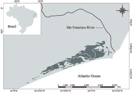
This study was conducted in the estuarine region of the São Francisco River (10°50’ S, 36°44’ W), which comprises an area of approximately 3531.16 ha (35.31 km2) covered by mangrove forests (Figure 1). The studied

area is crossed by a network of tidal channels fringed by mangrove forests characterized by a high structural variability, with average height and diameter at breast height (DBH) ranging from 4.34 to 8.36 m and 4.59 to 8.66 cm, respectively (SANTOS et al., 2012). These mangrove forests are composed by Avicennia schaueriana, A. germinans, Laguncularia racemosa and R. mangle, with the later species being the dominant one (relative dominance > 60%) (SANTOS et al., 2012).

Figure 1. Map of the study area (Datum WGS 84). Mangrove cover was obtained from the database

of the Brazilian Ministry of the Environment and is indicated with dark grey.

Sampling Design

The sampling method was adapted from NOVELLI; CINTRÓN (1986), SOARES; SCHAEFFER-NOVELLI (2005), BURGER; DELITTI (2008), and SAMPAIO et al. (2010).

Seeking to achieve a balance between sample representativeness per size range, the sampling efort needed to collect each individual, the negative impact caused by the felling of larger trees and the positive impact of the inclusion of a greater number of individuals in model itting, the following sampling strategy was deined: 1) DBH < 13 cm: four trees per 1-cm class; 2) DBH > 13.1 cm: two trees per 2-cm class. The higher size class as deined based on the phytosociological assessment of SANTOS et al. (2012). Based on this sampling strategy, 74 trees were felled. For each tree, the following variables were measured before sampling: diameter at breast height or above the highest prop root; height; mean diameter of the crown; and crown area, which was determined assuming an elliptical shape, as follows: crown area = (π × d₁ × d₂) / 4, where d₁ and d₂ are the ellipse diameters measured by crown projection on the ground (SOARES; SCHAEFFER-NOVELLI, 2005).

After size measurements, the trees were felled. To measure the fresh biomass, each tree was separated manually into the following compartments (plant parts): leaves (including buds and stipules); reproductive parts (lowers, fruits, and propagules); twigs (diameter < 2.5

cm); branches (diameter > 2.5 cm); main branches; trunk; and prop roots. Main branches were sampled when the tree presented bifurcation right after the highest stilt root, but as long as the branches had similar sizes (SOARES; SCHAEFFER-NOVELLI, 2005). All material was weighed in the ield with dynamometer-type scales. Sub-samples of each compartment were taken to the laboratory to determine their dry weights.

Sample

Processing

and

Statistical

Treatment of Data

After the determination of the fresh mass, the sub-samples of each compartment were dried for 15 days at 70ºC. The dry weights of the samples were determined by precision scales (0.01 g). Simple linear regression analysis, using the STATISTICA 7.0 software and considering a signiicance level of 1%, was applied to determine the relationship between dry weights (dependent variable) and fresh weights (independent variable) of each compartment. The dry mass of each compartment was obtained by applying the fresh mass obtained in the ield to the regression equations. The dry mass of the whole tree was then obtained by summing the dry mass of each compartment.

data. The independent variables were deined according to SOARES; SCHAEFFER-NOVELLI (2005) and are presented in Table 1.

As dependent variables, in addition to those aforementioned, the following combinations of compartments were used according to the guidelines of SOARES; SCHAEFFER-NOVELLI (2005):

a) Green parts (Leaves + Reproductive parts); b) Crown 1 (Leaves + Reproductive parts + Branches); c) Crown 2 (Leaves + Reproductive parts + Twigs + Branches);

d) Crown 3 (Leaves + Reproductive parts + Branches + Main Branches);

e) Trunk + Main Branches;

f) Woody parts (Twigs + Branches + Main Branches + Trunk + Prop Roots);

g) Aerial parts (Total - Prop roots).

In the evaluation of the models, the basic assumptions of simple linear regression analysis were checked according to the recommendations of ZAR (2010); DRAPER; SMITH (1998). Normality and homogeneity of variances were veriied for each regression by residual analysis. The signiicance of each regression was evaluated by analysis of variance (ANOVA). The statistically signiicant regressions that met the assumptions of the test were analyzed for goodness of it by calculating the R²_a (adjusted coeicient of determination), for precision (standard error of estimation - SEE), and through graphical analysis of the dispersions.

Following the studies of BROWN et al. (1989), BROWN et al. (1997), ONYEKWELU (2004), SAH et al. (2004) and SOARES; SCHAEFFER-NOVELLI (2005), the criteria for selecting the best models were (a) highest R2

a, (b) lowest SEE, and (c) best graphical distribution of absolute residual values.

RESULTS

Seventy four trees were sampled, with DBH and height ranging from 0.95 to 39.18 cm and 0.74 to 22.52

m, respectively. The regressions between dry and fresh weights per compartment are all signiicant (Table 2) and presented R2

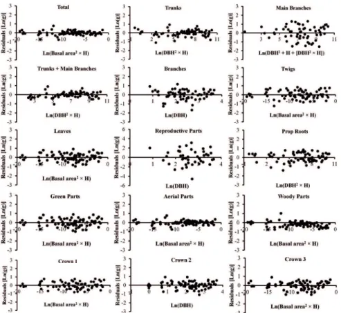
a between 0.91 and 0.97, which suggests good it of the equations. The dry weights of each tree (and its compartments) were thus estimated by applying the fresh weights to these regression equations. Considering all the combinations of dependent and independent variables and the two types of equations (ln-transformed or not), 375 linear allometric equations were tested. Most of the equations were signiicant (p<0.01), except for reproductive parts, which presented some equations that were not signiicant. The residual analysis showed that only the models that were under logarithmic transformation met the assumptions of normality and homoscedasticity. More than not meeting the assumptions of normality and homoscedasticity, most non-transformed equations presented an arc-shaped distribution of residuals, which is an indication that a curvilinear relationship between dependent and independent variables should be considered instead of a linear one (see ZAR, 2010). Nevertheless, in some cases the residuals of non-transformed equations presented a combination between arc-shaped distribution and a pattern characterized by the increase of the residuals variance with the increase of the independent variable, which indicates heteroscedasticity (i.e. Figure 2). On the other hand, log-transformed equations presented residuals that were linearly distributed over the independent variable range, as demonstrated by the best-it equations, indicating homoscedasticity (Figure 3). Log-transformed equations also showed better adjustment and lower standard errors. As a result, non-logarithmic equations were discarded.

The coeicients of determination (R2

a) and the standard errors of estimation (SEE) of all the log-transformed equations are presented in Table 3. Based on these results, the best allometric models by compartment and combination of compartments were determined and are presented in Table and Figure 4. The best models, the ones with the lowest SEE, also presented the highest R2

a. These models have coeicients of determination greater than 0.90 in most cases, except for main branches and

Table 1. Independent variables used to estimate the biomass of R. mangle according to the type of model. Legend: DBH in

cm; Height in m; Crown area in m2; Crown diameter in m; Basal Area in m2.

Type of Model Independent Variables (x)

y = a + bx DBH; Height; Crown Area; DBH × Height; Mean Crown Diameter; DBH2 × Height; (Basal Area)2 × Height;

DBH2 + Height + (DBH2 × Height); Basal Area; DBH2; Height2; (Crown Area)2; (Mean Crown Diameter)2;

(Basal Area)2; (DBH × Height)2; (DBH2 × Height)2, Basal Area × Height

ln(y) = a + bln(x) DBH; Height; Crown Area; DBH × Height; Mean Crown Diameter; DBH2 × Height; (Basal Area)2 × Height;

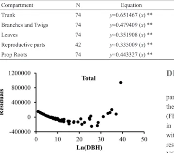
Table 2. Regressions between dry weights (g) and fresh weights (g) for each compartment of R. mangle. Legend: n=sample

size; y=dry weight; x=fresh weight; R2a=Adjusted Coeicient of Determination; Sb=Standard error of the coeicient of regression; SEE=Standard Error of Estimation; **=p<0.01.

Compartment N Equation R2

a Sb SEE

Trunk 74 y=0.651467 (x) ** 0.97 0.009046 394.005

Branches and Twigs 74 y=0.479409 (x) ** 0.94 0.013583 124.632

Leaves 74 y=0.351908 (x) ** 0.91 0.012867 161.0216

Reproductive parts 42 y=0.335009 (x) ** 0.96 0.010922 423.4881

Prop Roots 74 y=0.443327 (x) ** 0.93 0.014143 450.6888

Figure 2. Residuals distribution for the relationship between total

biomass and DBH.

reproductive parts, which showed maximum R2

a values of 0.85 and 0.43, respectively. The lower sample size for these compartments (main branches=60; reproductive parts=43) are probably one of the causes of this pattern, but seasonality may also play a role, as will be discussed in the next section.

Combinations of compartments showed high values of R2

a (see Tables 3 and 4), such as those related to aerial parts (R2

a=0.99) and woody parts (R2a=0.99), and may be considered good alternatives for estimating the biomass of the plant portions. In terms of independent variables, “Basal Area² × Height” and “DBH² × Height”, which simulate volume measures, stood out for generating the best equations for most of the dependent variables (Table 4). On the other hand, “Height”, “DBH × Height” and the variables related to measurements of the crown (mean diameter and area) had generally higher SEE and lower R2

a (Table 3) and were not related to any of the best-it equations.

Considering, that DBH is more easily measured at the ield and may have higher precision in forestry inventories then height, allometric equations considering only DBH as the predictor variable are alternatively presented in Table 5 and Figure 4 for practical reasons.

DISCUSSION

The fact that some equations tested for reproductive parts were not signiicant is probably explained by the seasonal nature of reproduction of this species (FERNANDES, 1999), which led to the sampling of trees in diferent phases of the reproduction cycle and thus with diferent proportions of reproductive tissues. Similar results were also obtained by SOARES; SCHAEFFER-NOVELLI (2005) for R. mangle and by ESTRADA et al. (2014) for A. schaueriana. Thus, considering that this factor would afect the variability of the biomass in that compartment, sampling should have always been done during the same reproductive phase, which would result in a logistically unfeasible sampling strategy.

It was found that the models with the greatest R2

a values showed the lowest SEEs for all compartments, including total biomass, unlike SOARES; SCHAEFFER-NOVELLI (2005), who found lower SEEs for some models that did not present maximum R2

a. Considering that the development of allometric models for biomass estimation assumes minimization of errors and maximized accuracy, it is desirable that the selected models present minimum SEE and maximum R2

a values. As presented before, the models that were under logarithmic transformation were the only ones to meet the assumptions of normality and homogeneity of variances and they also showed better adjustment and lower standard errors, which is in agreement with the indings of CLOUGH; SCOTT (1989), ONG et al. (2004), COMLEY; MAcGUINNESS (2005) and HOSSAIN et al. (2008). This pattern explains why the non-transformed equations were discarded from the analysis.

The lower R2

Figure 3. Residuals distribution for the best log-transformed equations (see Table 4).

SCHAEFFER-NOVELLI (2005) and ESTRADA et al. (2014), who found similar results for these compartments. For the reproductive parts, it should also be noted the seasonal behavior of this species with respect to its reproduction, as discussed earlier.

It was found that the grouping of compartments was advantageous in order to obtain equations for estimating the biomass of the plant portions, since they showed high values of R2

a (Table 4), such as those related to aerial parts (R2

a=0.99) and woody parts (R2a=0.99). The grouping of compartments showed to be a good way of minimizing the variances, the examples being reproductive parts and main branches, which presented increased adjustments when associated to other compartments than individually (Table 4).

Although DBH is generally the most common independent variable found in the available allometric models (CLOUGH; SCOTT, 1989; FROMARD et al., 1998; COMLEY; McGUINNESS, 2005; KOMYIAMA et al., 2008), it was observed that the equations based on “Basal Area² × Height” and “DBH² × Height” presented higher R2

a in most of the best equations in the present

study. Other studies have also found good its with these variables, such as TAMOOH et al. (2009), for R. mucronata in Gazi Bay (Kenya), SOARES; SCHAEFFER-NOVELLI (2005) for R. mangle and ESTRADA et al. (2014) for A. schaueriana in Guaratiba (Rio de Janeiro, Brazil), and MURALI et al. (2005), for deciduous species tropical forests. However, considering the recommendations of BURGER; DELITTI (2008), who claim that models using DBH as the independent variable have the advantages of being easily measured and having higher precision of measurement in the ield, equations considering only DBH are, alternatively, presented in Table 5.

The analysis of the data in Table 5 shows that the values of R2

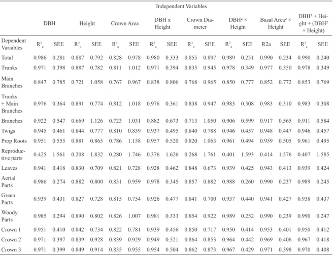
Table 3. Adjusted coeicients of determination (R2

a) and standard error of estimation (SEE) for all log-transformed regres -sion analyses.

Independent Variables

DBH Height Crown Area DBH x _Height Crown Dia_meter - DBH² × _Height Basal Area² × _Height DBH² + Height + (DBH²

-× Height) Dependent

Variables R2a SEE R2a SEE R2a SEE R2a SEE R2a SEE R2a SEE R2a SEE R2a SEE

Total 0.986 0.281 0.887 0.792 0.828 0.978 0.980 0.333 0.855 0.897 0.989 0.251 0.990 0.234 0.990 0.240

Trunks 0.971 0.398 0.887 0.782 0.811 1.012 0.971 0.394 0.835 0.945 0.978 0.349 0.977 0.350 0.978 0.349

Main

Branches 0.847 0.785 0.721 1.058 0.767 0.967 0.838 0.806 0.768 0.965 0.850 0.777 0.852 0.772 0.853 0.769

Trunks + Main

Branches 0.976 0.364 0.891 0.774 0.812 1.018 0.976 0.361 0.838 0.947 0.983 0.308 0.983 0.310 0.983 0.308

Branches 0.922 0.547 0.669 1.126 0.723 1.031 0.882 0.673 0.713 1.050 0.906 0.599 0.917 0.565 0.911 0.584

Twigs 0.945 0.461 0.844 0.777 0.810 0.859 0.937 0.495 0.840 0.788 0.946 0.457 0.948 0.447 0.946 0.457

Prop Roots 0.951 0.555 0.881 0.865 0.786 1.158 0.957 0.520 0.820 1.063 0.961 0.494 0.959 0.505 0.961 0.495

Reproduc

-tive parts 0.425 1.561 0.208 1.832 0.280 1.746 0.376 1.626 0.268 1.761 0.401 1.593 0.414 1.576 0.407 1.585

Leaves 0.941 0.418 0.830 0.709 0.821 0.728 0.928 0.462 0.848 0.673 0.939 0.425 0.943 0.413 0.939 0.424

Aerial

Parts 0.986 0.274 0.882 0.800 0.831 0.959 0.978 0.345 0.857 0.882 0.988 0.260 0.990 0.237 0.989 0.245

Green

Parts 0.939 0.431 0.827 0.728 0.815 0.754 0.926 0.477 0.841 0.700 0.937 0.440 0.941 0.427 0.938 0.437

Woody

Parts 0.985 0.294 0.890 0.802 0.826 1.007 0.981 0.333 0.854 0.922 0.989 0.252 0.990 0.239 0.990 0.247

Crown 1 0.951 0.410 0.842 0.734 0.822 0.781 0.939 0.456 0.850 0.717 0.950 0.414 0.953 0.401 0.950 0.412

Crown 2 0.971 0.397 0.839 0.928 0.839 0.929 0.949 0.521 0.864 0.853 0.964 0.442 0.969 0.406 0.967 0.418

Crown 3 0.971 0.399 0.849 0.914 0.835 0.955 0.954 0.504 0.862 0.873 0.967 0.429 0.971 0.398 0.970 0.408

The R2

a of the selected equations produced in the present study are higher than those observed by MEDEIROS; SAMPAIO (2008) for the same species in the mangroves of Itamaracá (Pernambuco, Brazil - 7° S): leaves=0.83; branches=0.90; trunk=0.89; prop roots=0.85; total=0.94. This diference is probably due to the higher sampling efort used in this study, since MEDEIROS; SAMPAIO (2008) used a smaller sample size (36 individuals, against 74 individuals in this study) and sampled trees with smaller diameter (2.5 to 20.7 cm) and height (1.8 to 14.0 m) ranges. Therefore, given the greater accuracy and representativeness in terms of size amplitude, the models developed in this study are more suitable for estimating the aboveground biomass of R. mangle in Northeastern Brazilian mangroves as well as in other regions with a similar environmental setting in the mid-tropical (5-15° S and N) coasts of the Atlantic and East Paciic region.

The logarithmic models generated the best its for the relationships between biomass and the independent variables. The selected independent variables for this study explained, in most cases, over 90% of the variability of the aboveground biomass of R. mangle trees. The variables Basal Area² × Height, and DBH² × Height, led to equations with the lowest SEEs and the best its in most compartments.

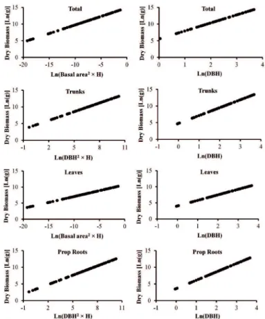
Figure 4. Graphical dispersions of the best log-transformed equations and the alternative DBH-only

equations for the main dependent variables (Total biomass; Trunks; Leaves; and Prop Roots).

Table 4. Best allometric models for estimation of the aboveground biomass of R. mangle. Legend: H=height; n=sample number; a and b=intercept and coeicient of regression, respectively; R2

a=adjusted coeicient of determination; F=ANOVA F value; SEE - standard error of estimation.

Model Compartment n a b R2

a F SEE

Ln (biomass) = a + b Ln (DBH2 × H) Trunk 74 4.160747 0.875996 0.98 3179.580 0.349

Ln (biomass) = a + b Ln [DBH2 + H + (DBH2 × H)] Main branches 60 1.914396 0.891536 0.85 342.9470 0.769

Ln (biomass) = a + b Ln (DBH) Branches 64 3.157351 2.638149 0.92 746.0843 0.547 Ln (biomass) = a + b Ln (Basal area2 × H) Twigs 74 11.309867 0.420531 0.95 1343.560 0.447

Ln (biomass) = a + b Ln (Basal area2 × H) Leaves 74 10.712324 0.366420 0.94 1197.919 0.413

Ln (biomass) = a + b Ln (DBH) Reproductive _parts 43 -0.456055 2.119786 0.43 32.06745 1.560

Ln (biomass) = a + b Ln (DBH2 × H) Prop roots 74 2.939739 0.934209 0.96 1799.216 0.494

Ln (biomass) = a + b Ln (Basal area2 × H) Total 74 14.86763 0.51320 0.99 7313.432 0.234

Ln (biomass) = a + b Ln (Basal area2 × H) Green parts 74 10.805191 0.372766 0.94 1159.572 0.427

Ln (biomass) = a + b Ln (Basal area2 × H) Aerial parts 74 14.599081 0.507845 0.99 7007.320 0.237

Ln (biomass) = a + b Ln (Basal area2 × H) Crown 1 74 11.761324 0.395483 0.95 1476.419 0.401

Ln (biomass) = a + b Ln (DBH) Crown 2 74 4.409862 2.346133 0.97 2412.159 0.397 Ln (biomass) = a + b Ln (Basal area2 × H) Crown 3 74 13.753848 0.507336 0.97 2472.099 0.398

Ln (biomass) = a + b Ln (Basal area2 × H) Woody parts 74 14.898165 0.526360 0.99 7365.104 0.239

Ln (biomass) = a + b Ln (DBH2 × H) Trunks + Main

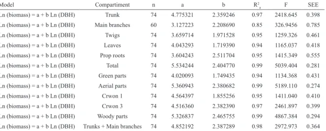
Table 5. Allometric models to estimate the aboveground biomass of R. mangle considering only DBH as the independent

variable. Legend: n=sample number; a and b=intercept and coeicient of regression, respectively; R2

a=adjusted coeicient of determination; F=ANOVA F value; SEE - standard error of estimation.

Model Compartiment n a b R2

a F SEE

Ln (biomass) = a + b Ln (DBH) Trunk 74 4.775321 2.359246 0.97 2418.645 0.398 Ln (biomass) = a + b Ln (DBH) Main branches 60 3.127223 2.208690 0.85 326.9456 0.785 Ln (biomass) = a + b Ln (DBH) Twigs 74 3.659714 1.971528 0.95 1259.326 0.461 Ln (biomass) = a + b Ln (DBH) Leaves 74 4.043293 1.719390 0.94 1165.037 0.418 Ln (biomass) = a + b Ln (DBH) Prop roots 74 3.604243 2.511704 0.95 1415.349 0.555 Ln (biomass) = a + b Ln (DBH) Total 74 5.534244 2.404770 0.99 5039.404 0.281 Ln (biomass) = a + b Ln (DBH) Green parts 74 4.020093 1.749435 0.94 1134.368 0.431 Ln (biomass) = a + b Ln (DBH) Aerial parts 74 5.360943 2.380682 0.99 5189.110 0.274 Ln (biomass) = a + b Ln (DBH) Crwon 1 74 4.564397 1.855256 0.95 1411.040 0.410 Ln (biomass) = a + b Ln (DBH) Crwon 3 74 4.516360 2.382390 0.97 2461.897 0.399 Ln (biomass) = a + b Ln (DBH) Woody parts 74 5.326837 2.465755 0.99 4867.384 0.294 Ln (biomass) = a + b Ln (DBH) Trunks + Main branches 74 4.852192 2.387289 0.98 2972.973 0.364

ACKNOWLEDGEMENTS

This work was supported through a research grant conceded from PETROBRAS – Petróleo Brasileiro to Francisco Sandro Rodrigues Hollanda.

REFERENCES

ABOHASSAN, R. A. A.; OKIA, C. A.; AGEA, J. G.; KIMOND, J. M.; MCDONALD, M. M. Perennial biomass production in arid mangrove system on the red sea cost of Saudi Arabia.

Environ. Res. J., v. 6, n. 1, p. 22-31, 2012.

ALONGI, D. M. Paradigm shifts in mangrove biology. In: PERILLO, G.; WOLANSKI, E.; CAHOON, D.; BRINSON, M. (Eds.). Coastal wetlands: An integrated ecosystem approach. Amsterdam: Elsevier, 2009. p. 615-634.

BROWN, S. Measuring carbon in forests: current status and future challenges. Environ. Pollut., v. 116, n. 3, p. 363-372, 2002.

BROWN, S.; GILLESPIE, A. J. R.; LUGO, A. E. Biomass estimation methods for tropical forests with applications to forest inventory data. For. Sci., v. 35, n. 4, p. 881-902, 1989.

BROWN S.; SCHROEDER, P.; BIRDSEY, R. Aboveground biomass distribution of US eastern hardwood forests and the use of large trees as an indicator of forest development. For. Ecol. Manag., v. 96, n. 1-2, p. 37-47, 1997.

BURGER, D. M.; DELITTI, W. B. C. Allometric models for estimating the phytomass of a secondary Atlantic Forest area of southeastern Brazil. Biota Neotrop., v. 8, n. 4, p. 131-136,

2008.

CHANDRA, I. A.; SECA, G.; HENA, M. K. A. Aboveground biomass production of Rhizophora apiculata Blume in

Sarawak mangrove forest. Am. J. Agric. Biol. Sci., v. 6, n. 4,

p. 469-474, 2011.

CLOUGH, B. F.; SCOTT, K. Allometric relationships for estimating above-ground biomass in six mangrove species.

For. Ecol. Manag., v. 27, n. 2, p. 117-127, 1989.

COMLEY, B. W. T.; MCGUINNESS, K. A. Above- and below-ground biomass, and allometry of four common northern Australian mangroves. Aust. J. Bot., v. 53, n. 5, p. 431-436,

2005.

COX, E. F.; ALLEN, J. A. Stand structure and productivity of the introduced Rhizophora mangle in Hawaii. Estuaries, v. 22, n.

2, p. 276-284, 1999.

DONATO, D. C.; KAUFFMAN, J. B.; MURDIYARSO, D.; KURNIANTO, S.; STIDHAM, M.; KANNINEN, M. Mangroves among the most carbon-rich forests in the tropics.

Nat. Geosci., v. 4, p. 293-297, 2011.

DRAPER, N. R.; SMITH, H. Applied Regression Analysis. 3rd ed.

New York: John Wiley and Sons, 1998. 736 p.

DUKE, N. C. Mangrove Floristics and Biogeography. In: ROBERTSON, A. I.; ALONGI, D. M. (Eds.). Tropical Mangrove Ecosystems, Coastal and Estuarine Studies 41.

Washington: American Geophysical Union Press, 1992. p. 63-100.

DUKE, N. C.; LO, E.; SUN, M. Global distribution and genetic discontinuities of mangroves – emerging patterns in the evolution of Rhizophora. Trees, v. 16, n. 2, p. 65-79, 2002.

ESTRADA, G. C. D.; SOARES, M. L. G.; SANTOS, D. M. C.; FERNANDEZ, V.; ALMEIDA, P. M. M.; ESTEVAM, M. R. M.; MACHADO, M. R. O. Allometric models for aboveground biomass estimation of the mangrove Avicennia schaueriana. Hydrobiologia, v. 734, n. 1, p. 171-185, 2014.

FERNANDES, M. E. B. Phenological patterns of Rhizophora

L., Avicennia L. and Laguncularia Gaertn. F. in Amazonian

mangrove swamps. Hydrobiologia, v. 413, p. 53-62, 1999.

FROMARD, F.; PUIG, H.; MOUGIN, E.; MARTY, G.; BETOULLE, J. L.; CADAMURO, L. Structure, above-ground biomass and dynamics of mangrove ecosystems: new data from French Guiana. Oecologia, v. 115, n. 1, p. 39-53, 1998.

KOMIYAMA, A.; ONG, J. E.; POUNGPARN, S. Allometry, biomass, and productivity of mangrove forests: A review.

Aquat. Bot., v. 89, n. 2, p. 128-137, 2008.

LU, D.; MAUSEL, P.; BRONDIZIO, E.; MORAN, E. Assessment of atmospheric correction methods for Landsat TM data applicable to Amazon basin LBA research. Int. J. Remote. Sens., v. 23, n. 13, p. 2651-2671, 2002.

MCLEOD, E.; CHIMURA, G. L.; BOUILLON, S.; SALM, R.; BJÖRK, M.; DUARTE, C. M.; LOVELOCK, C. E.; SCHLESINGER, W. H.; SILLIMAN, B. R. A blueprint for blue carbon: toward an improved understanding of the role of vegetated coastal habitats in sequestering CO2. Front. Ecol.

Environ., v. 9, n. 10, p. 552-560, 2011.

MEDEIROS, T. C. C.; SAMPAIO, E. V. S. B. Allometry of aboveground biomasses in mangrove species in Itamaracá, Pernambuco, Brazil. Wetl. Ecol. Manag., v. 16, n. 4, p.

323-330, 2008.

MURALI, K. S.; BHAT, D. M.; RAVINDRANATH, N. H. Biomass estimation equations for tropical deciduous and evergreen forests. Int. J. Agric. Resour. Gov. Ecol., v. 4, n. 1,

p. 81-92, 2005.

ONG, J. E.; GONG, W. K.; WONG, C. H. Allometry and partitioning of the mangrove, Rhizophora apiculata. For. Ecol. Manag., v. 188, n. 1-3, p. 395-408, 2004.

ONYEKWELU, J. C. Above-ground biomass production and biomass equations for even-aged Gmelina arborea (ROXB)

plantations in south-western Nigeria. Biom. Bioen., v. 26, n.

1, p. 39-46, 2004.

ROSS, M. S.; RUIZ, P. L.; TELESNICKI, G. J.; MEEDER, J. F. Estimating above-ground biomass and production in mangrove communities of Biscayne National Park, Florida (U.S.A.). Wetl. Ecol. Manag., v. 9, n. 1, p. 27-37, 2001.

SAH, J. P.; ROSS, M. S.; KOPTUR, S.; SNYDER, J. R. Estimating aboveground biomass of broadleaved woody plants in the understory of Florida Keys pine forests. For. Ecol. Manag., v. 203, n. 1-3, p. 319-329, 2004.

SAMPAIO, E.; GASSON, P.; BARACAT, A.; CUTLER, D.; PAREYN, F.; LIMA, K. C. Tree biomass estimation in regenerating areas of tropical dry vegetation in northeast Brazil. For. Ecol. Manag., v. 259, n. 6, p. 1135-1140, 2010.

SANTOS, T. O.; ANDRADE, K. V. S.; SANTOS, H. V. S.; CASTANEDA, D. A. F. G.; SANTANA, M. B. S.; HOLANDA, F. S. R.; SANTOS, M. J. C. Caracterização estrutural de bosques de mangue: Estuário do rio São Francisco. Sci. Plena, v. 8, n. 4, p. 1-7, 2012.

SCHAEFFER-NOVELLI, Y.; CITRÓN, G. Guia para estudo de

áreas de manguezal: estrutura, função e lora. São Paulo: Caribbean Ecological Research, 1986. 150 p.

SHERMAN, R. E.; FAHEY, T. J.; MARTINEZ, P. Spatial patterns of biomass and aboveground net primary productivity in a mangrove ecosystem in the Dominican Republic. Ecosystems,

v. 6, n. 4, p. 384-398, 2003.

SIIKAMÄKI, J.; SANCHIRICO, J. N.; JARDINE, S. L. Global economic potential for reducing carbon dioxide emissions from mangrove loss. Proc. Natl. Acad. Sci. U.S.A., v. 109, n.

36, p. 14369-14374, 2012.

SILVEIRA, P.; KOEHLER, H. S.; SANQUETTA, C. R.; ARCE, J. E. O estado da arte na estimativa de biomassa e carbono em formações lorestais. Floresta, v. 38, n. 1, p. 185-206, 2007.

SMITH III, T. J.; WHELAN, K. R. T. Development of allometric relations for three mangrove species in South Florida for use in the Greater Everglades Ecosystem restoration. Wetl. Ecol. Manag., v. 14, n. 5, p. 409-419, 2006.

SOARES, M. L. G.; SCHAEFFER-NOVELLI, Y. Above-ground biomass of mangrove species. I. Analysis of models. Estuar. Coast. Shelf Sci., v. 65, n. 1-2, p. 1-18, 2005.

SOARES, M. L. G.; ESTRADA, G. C. D.; FERNANDEZ, V.; TOGNELLA, M. M. P. Southern limit of the Western South Atlantic mangroves: Assessment of the potential efects of global warming from a biogeographical perspective. Estuar. Coast. Shelf Sci., v. 101, p. 44-53, 2012.

TAMOOH, F.; KAIRO, J. G.; HUXHAM, M.; KIRUI, B.; MENCUCCINI, M.; KARACHI, M. Biomass accumulation in a rehabilitated mangrove forest at Gazi Bay. In:

HOORWEG, J.; MUTHIGA, N. (Eds.). Advances in Coastal – People, process and ecosystems in Kenya. Leiden:African

Studies Centre, 2009. p. 138-147.

TWILLEY, R. R.; CHEN, R. H.; HARGIS, T. Carbon sinks in mangroves and their implications to carbon budget of tropical coastal ecosystems.

Water Air Soil Pollut., v. 64, n. 1, p. 265-288, 1992.