Purchasing power parity: Evidence of long memory processes and fractional integration

Contents lists available at GrowingScience

Decision Science Letters

homepage: www.GrowingScience.com/dsl

Purchasing power parity: Evidence of long memory processes and fractional integration

Nadhem Selmi* _{and Nejib Hachicha}

Department of Quantitative Methods, Faculty of Economics and Management of Sfax - Tunisia

C H R O N I C L E A B S T R A C T

Article history:

Received December 10, 2014 Received in revised format: March 2, 2015

Accepted March 2, 2015 Available online March 2 2015

The Purchasing Power Parity (PPP) theory, which serves as a key to the determination of several models of exchange rates, suggests a long-term relationship between exchange rates and relative prices. It states that the price levels in all the countries are the same when measured in terms of a single currency. The purpose of this study is to model the behavior of the exchange rates of five partner countries of Tunisia, namely, (Germany, the United States, France, Italy, the UK, Morocco and Libya) relative to its fundamentals over the period 1990-1999. Beyond the traditional linear cointegration, we use the approaches based on fractional cointegration. We are trying to discriminate between the adjustment dynamics with long memory (but linear) and a dynamics of a short memory (nonlinear). Given the important role of the exchange rates in the successful experience of open economies, we are interested, in this work, in analyzing the dynamics of the exchange rates in the long run. The econometric results obtained through the GPH tests, make us consider the PPP as an event in the long run if significant short-term deviations from the PPP cannot exist. Therefore, the analysis of the fractional cointegration makes the deviations, regarding equilibrium, follow a slightly integrated process and therefore capture a much wider group of research parity or mean-reverting behavior.

Growing Science Ltd. All rights reserved. 5

© 201

Keywords:

Exchange rate Linear cointegration Fractional cointegration

1. Introduction

The equilibrium exchange rate is defined as the rate that allows for both internal and external balance of trade balance. Several theories seek to determine this rate as the theory of interest rate parity and the quantity theory of money. However, the theory of Purchasing Power Parity (PPP) remains the basic theory as it was introduced by Frenkel (1978), Dridi and Kugler (1995). PPP is a very important concept in international economic modeling; it is used for important goals and specific. Indeed, it serves as a guide to monetary authorities when they intervene in the foreign exchange market to move the exchange rate to a level consistent in equilibrium. The deviation of the exchange rate market given by the theory of PPP can result in either overvalued or undervalued currency. These two phenomena, and on the undervaluation may have adverse effects on exports, imports and the unemployment rate.

* Corresponding author.

398

Ben Ayed (1984), Abuaf and Jorion (1990), Ariff and Bahamushah (1997), Taylor (1999), Caner and Kilian (2001) and Mark (2003) studied the parity of purchasing power based on both absolute and relative versions. The absolute version was tested by regression of the nominal exchange rate on the ratio of domestic and foreign prices. But check this absolute version requires the completion of several assumptions, where the use relative version of the PPP as it is introduced by Fisher and Park (1991) and Glen (1992). This version is checked on the regression of the real exchange rate on the order of auto-regression for each country studied.

In the past numerous studies on real exchange rate adjustment to Purchasing Power Parity (PPP) under different nominal exchange rate regimes, no agreement has been reached. On the one hand, some studies establish that the mean-reverting of real exchange rate below the fixed exchange rate regime is more pronounced than under the flexible exchange rate regime (e.g. Mussa, 1986; Parsley & Popper, 2001). On the other hand, some recent studies found weaker evidence of mean-reverting of real exchange rate for many euro markets under the euro regime, which represents an extreme form of fixed exchange rate, than under the regimes by more flexible exchange rate (See for example, Rogers, 2007; Christidou & Panagiotidis, 2010; Wu & Lin, 2011). In addition, there are also works showing no clear-cut difference in the mean-reverting behavior of real exchange rates across fixed and flexible nominal exchange rate regimes (See for instance, Grilli & Kaminsky, 1991; Lothian & Taylor, 1996; Bissoondeeal, 2008), between many others.

How integrated are international countries? Recent advances in the purchasing power parity literature reveal that price based answers to this question depend on factors that vary across time, space, and products. While several research has generated important insights into long-run deviations in the Law of One Price across markets (Froot & Rogoff, 1995; Rogoff, 1996; Goldberg & Knetter, 1997; Taylor & Taylor, 2004; Crucini & Yilmazkuday, 2013), long-run PPP especially weak-form and strong-form PPP remains less than fully understood. This gap remains particularly salient among developed and developing markets. Rogoff (1996), especially, expressed concern about whether PPP holds among developed and developing countries.

Empirical literature, including Michael et al. (1997), Obstfeld and Taylor (1997), Sarantis (1999), Sarno et al. (2004), and Bec et al. (2010), have made use of nonlinear threshold-type autoregressive models to examine the PPP persistence puzzle, a notion indicated in a survey through Rogoff (1996). The inspiration for using nonlinear models in this situation is that the original empirical studies used to establish the puzzle may have arisen due to process misspecification.

The objective of this paper is to test the theory of purchasing power parity in distinguishing these two main versions absolute and relative, and indicate both the non-validity of the PPP: the overvaluation and undervaluation of currency. In the empirical part we will estimate the nominal exchange rate on the ratio of domestic and foreign prices and the real exchange rate on the order autoregressive using Box-Jenkins techniques for each country while indicating the nature of each process. Finally, we will test the fractional integration parameter.

2. Econometric methodology

We defineε_t, t =1, 2,....as a stationary process with a density which is positive and finite. In this context the processy_t, integrated of order d is defined by:

(

1−L

)

d y_t =ε_t t=1, 2,....

With the process ε_t ARMA is likely stationary, invertible covariance with an exponentially decreasing. - for d =0, y_t =ε_t so ‘‘low autocorrelation’’.

- for −0.5< <d 0, the process is anti-persistent and has a short memory, the autocorrelations decrease hyperbolically to zero.

- for 0< <d 0.5, y_tis stationary long memory but auto-covariance order j down very slowly because of the term _k2d−1

for k→ ∞because we :

( ) (

)

( ) (

)

2 0 1 2 2 1

lim 1 d k k f d k d d

γ σ −

→∞

 Γ − 

= _{ }

Γ − Γ −

 

 

(1)

where

( )

1 2

1 2 1 .... 0 1 .... q p

f θ θ θ

ϕ ϕ ϕ

− − − − =

− − − −

(2)

The distinction between process I d

( )

for different values of « d » is also important from an economic

standpoint: if a variable follows a I d

( )

for d∈

[

0.5,1

]

that may be no stationary. Robinson (1994) proposes a LM test for testing the unit root against the alternative fractional. The null hypothesis can be written as:

0: 0

H θ = (3)

of model

t t t

h =β′z +y t=1, 2,.... (4)

with

(

1−L

)

d+θ y_t =ε_t t=1, 2,.... (5)

where z_tis the vector of deterministic components of dimensions

(

k×1

)

this may include that z_tmay

be such that (z_t =1) where (z_t =

( )

1,t ′), test score is written in the form : 1 1 2 2 2 ˆ ˆ ˆ ˆ T

r A a

σ −     =  _{ }   (6)

where Tis the size of the sample. In addition,

( ) ( ) ( )

1

1

1 2

ˆ ;ˆ

T

j j j

j

a g I

T

π −_{ψ λ λ τ − λ}

=

= −

∑

(7)

( )

( ) ( )

( ) ( )

1

( ) ( )

1 ₂ 1 1 1

1 1 1 1

2

ˆ T T _ˆ T _{ˆ ˆ} T _ˆ

j j j j j j j

j j j j

A

T ψ λ ψ λ ε λ ε λ ε λ ε λ ψ λ

− − − − − = = = =  _{′ ′}    = − _{ }  _{ }  

∑

∑

∑

∑

 (8)

( )

1

( ) ( )

₁

2 2

1

2

ˆ ˆ ;ˆ

T j j j g I T π

σ σ τ − λ τ − λ

=

= =

∑

(9)

( )

log 2sin 2

j j

λ

ψ λ = (10)

( )

(

)

ˆ _j logg _j;ˆ

ε λ λ τ τ

∂ =

∂

(11)

whereI

( )

λ_j is the periodogram of the process :

(

)

ˆ

ˆ_t 1 L d y_t w_t

400

point _j 2 j

T π λ =

with

(

)

1

1 1

ˆ T T ₁ d

t t t t

t t

w w w L y

β

−

= =

 _′

=_{ } −



∑



∑

and

(

1

)

d

t t

w = −L z (13)

Robinson (1994) showed that rˆ→N

( )

0,1 for T → ∞, for the test unilateral H1:θ >0is given by the rule ‘‘reject H0 if ˆr >z_α’’at

α

% _{and conversely for the alternative} H₁:θ <0 is given by the rule ‘‘reject H0 if ˆr< −z_α’’. So the test case is written in the general form:

0

1 2 : 0

: pour 0

a

H

H T

θ

θ δ δ

= 



 = ≠



(14)

We introduce the following fractional cointegration. The vector X_tof size

(

n×1

)

fractionally cointegrated says d b, recordedX_t →CI d b

(

,

)

, if all components are integrated of order d such that

( )

it

X →I d and there is a non-zero vector r as N_t =r X′ _t is integrated of order

(

d b−

)

forb>0. In the general case of fractional cointegretion, the order of integration is defined for each. In the general case of fractional cointegration, the order of integration for each series is defined as

(

1, 2,..., ,

)

t n

X →CI d d d b . If for all ithen there exist a vector as

where:

(15)

and

(16)

In what follows we assume that only two components . Cheng and Lai (1993)

studied the case of fractional cointegration, and showed that the OLS estimator is better and converges to the different possible cases of cointegration order. In particular, they showed that under the general hypothesis of cointegration of order d, b such that d >0.5 et b>0, the OLS estimator is efficient and converges with a rate Tb d− . Robinson (1994) univariate test was used to test the order of integration errors:

1 ˆ 2

t t t

e =X −αX pour t=1, 2,.... (17)

where ˆα is the estimator of the cointegrating parameter by OLS. Using the same test statistic distribution normal limit, we can consider the model:

(

1−L

)

d+θe_t =v_t pour t =1, 2,.... (18)

where v_t is a process I

( )

0 , we test:

0: 0

H θ = (19)

against the alternative

1: 0

H θ < (20)

( )

it i

X →I d r≠0 N_t =r X′ _t →I d

( )

(

)

1

max _i

i n

d d b

≤ ≤

= −

1 1

max _i min _i i n i n

b d d

≤ ≤ ≤ ≤

 ₋ 

 

 



t

The test statistic rˆ asymptotically distribution N

( )

0,1 . If the null hypothesis is rejected against the alternative that implies that X_1t et X_2t fractionally cointegrated are called.

The error equilibrium has a smaller range than the original level of integration. However, as errors equilibrium are not actually observed are obtained minimizing the variance of the residuals of the regression, in finite samples of the residual series can be biased toward the stationary and therefore we expect the rejection of the null hypothesis.

For simplicity, we consider two series X_t and Y_t, both integrated of order 1, in other words, ∆X_t et

t

Y

∆ are stationary. As we have seen previously, X_t and Y_t are fractionally cointegrated if there is a cointegration relationship:

t t t

Y = +α βX +z (21)

where z_tis a fractionally integrated process. The test of resides was then implemented for the purpose of testing the null hypothesis:

0:

H X_t and Y_t are not cointegrated, that is to say z_tis integrated in order 1, for allα β, ∈IR. against the alternative:

1:

H X_t andY_t are cointegated, that is to say z_tis integrated in order, d, with d <1. These tests are applied to the estimated residuals of the long-term relationship:

ˆ ˆ

ˆ_{t t t}

z = − −Y α βX (22)

The asymptotic distribution under the null hypothesis is not known if the real errors z_t are observable. The search for fractional cointegration has been the subject of various studies focusing on financial time series and using mostly the method Geweke and Porter-Hudak (1983).

The fractional cointegration test of Robinson (1994) followed a similar problem in the cointegration test of Engle and Granger (1987) and Cheung and Lai (1993) for the regression fallacy. To negotiate this problem we obtain the empirical dimension of the cointegration test samples done using a simulation approach.

3. Data and summary statistics

Financial series considered are formed by the indices nominal exchange rate, the real exchange rate and price indices of general consumption French Franc / Dollar U.S, dinar Tunisian / Dollar U.S, British Pound / Dollar U.S, Italian Lira / Dollar U.S. German Deutschmark / Dollar U.S, Moroccan Dirham / Dollar U.S and Libyan Dinar / Dollar U.S. The data are monthly. The period of analysis for indices exchange rate from January 1990 to December 2006 for all series that is to say 204 observations. Price indices for general consumption, the period begin in January 1990 and ending in June 2006 for all series that is to say 198 observations.

Table 1

Descriptive statistics of the real exchange rate

402

The descriptive statistics show that an average series, the exchange rate is close to 2. Developed markets are characterized by a lower variance compared to emerging markets. Skewness is nonzero and positive for most of the series reflecting the asymmetric behavior of the series studied (except for Italy and Libya). The kurtosis is much higher than the normal value exposing the occurrence of extreme values and the existence of heteroscedasticity in the series. We also note the presence of serial autocorrelation of first and second order. These linear dependencies confirm the imperfect markets. The auto-correlation of the second order also explains the heteroscedasticity series yields (Table 1).

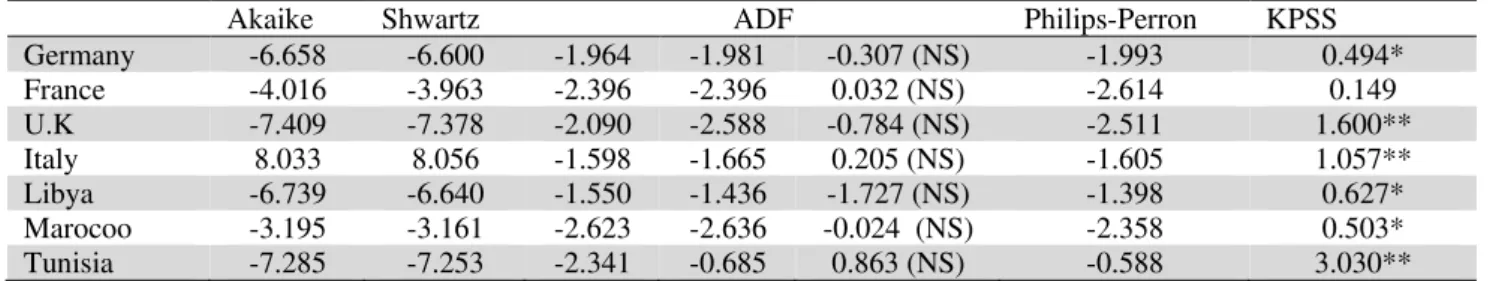
Table 2 Unit root Tests

Akaike Shwartz ADF Philips-Perron KPSS Germany -6.658 -6.600 -1.964 -1.981 -0.307 (NS) -1.993 0.494* France -4.016 -3.963 -2.396 -2.396 0.032 (NS) -2.614 0.149 U.K -7.409 -7.378 -2.090 -2.588 -0.784 (NS) -2.511 1.600** Italy 8.033 8.056 -1.598 -1.665 0.205 (NS) -1.605 1.057** Libya -6.739 -6.640 -1.550 -1.436 -1.727 (NS) -1.398 0.627* Marocoo -3.195 -3.161 -2.623 -2.636 -0.024 (NS) -2.358 0.503* Tunisia -7.285 -7.253 -2.341 -0.685 0.863 (NS) -0.588 3.030** Note : NS indicates that the process is non-stationary. * And ** indicate significant value is respectively to 10% and 5%.

The application of unit root tests (Table 2) the series reveals the presence of a unit root in all series level. The test results confirm those obtained Phillips Perron tests using Augmented Dickey-Fuller and remaining relatively stable number of delays used: presence of a unit root for the series in levels and stationary for the series in first difference.

The model is estimated ARFIMA (p, d, q) by the method of Geweke and Porter-Hudak (1983). From Table 3 can take the values of differentiation estimated for the countries studied.

Table 3

Estimation and test of long memory

Germany France U.K Italy Libya Marocoo Tunisia GPH1 0.280

(0.383) 0.160 (0.383) 0.218 (0.223) 0.157 (0.467) -40.038 (0.325) 0.207 (0.392) 0.025 (0.177) GPH2 0.082

(0.317) 0.118 (0.372) -0.059 (0.183) 0.453 (0.469) -0.057 (0.163) 0.031 (0.262) 0.058 (0.151) GPH3 0.032

(0.258) -0.127 (0.278) -0.062 (0.157) 0.272 (0.377) -0.057 (0.163) 0.132 (0.245) 0.0013 (0.147) RGSE1 -0.028 -0.087 -0.003 0.0625 -0.086 -0.144 0.013 RGSE2 -0.016 -0.076 -0.024 0.0499 -0.056 -0.095 -0.0105 RGSE3 -0.011 -0.024 0.064 0.127 -0.067 0.012 0.035 Whittle -0.045

(0.02) -0.077 (0.965) 0.0211 (0.997) 0.073 (0.00) -0.162 (0.964) -0.036 (0.960) 0.0264 (0.996) H 0.73 0.79 0.563 0.801 0.834 0.703 0.716 R/S Modifiée (V) 1.192 0.977 1.480 1.413 1.249 1.169 1.038 Note : H is the Hurst statistic estimated using the R/S method. GPH1, GPH2 and GPH3 represent the values of Geweke and Porter-Hudak for cases (u=0.45), (u=0.50) et (u=0.55). RGSE1, RGSE2 and RGSE3 represent respectively estimators Robinson (1995) for the cases of (u=0.75),(u=0.80)and (u=0.90). For each series appears on the first line the estimated fractional integration parameter, the value of the Student statistic is given in parentheses on the second line. Values in parentheses are the standard deviations of the estimated parameters and values brackets are t-statistics.

Test of fractional integration parameter

The test of Geweke and Porter-Hudak (1983) can also be used as a unit root test. Under the null hypothesis, the first order differentiated data follow a stationary ARMA process with d = 0. Thus, the unit root hypothesis can be tested by determining if data disaggregated with first order d is then significantly different from zero. So the GPH test provides a perspective for the study of the unit root hypothesis. Examination of residual autocorrelations series of processes studied allows us to incorporate some moving average in the specification process and thus lead to a global model of type ARMA (p, q).

We note that all the estimated parameters are statistically significant; the fractional differencing parameter between 0 and 1 is also statistically significant. In fact, we adopted a nonparametric test known test Geweke and Porter-Hudak (1983) in order to test the presence of long memory, the results of this test indicate that the processes are integrated of order fraction with

( )

ˆ _0.5

ˆ var

c d

t

d

−

= (23)

Student's t test also shows that the estimator of the parameter of fractional integration is statistically significant indicates that it is the evidence of short-term memory for the exchange rates of the countries studied. It is necessary not only to test the presence of unit root, but also to test short-term memory or long memory, and therefore consider a more general class of models where we consider the fractional differencing parameter, should not be restricted to integer values 1 or 0.

The fractional differentiation parameter is not 0, and it is less than one, where evidence of short-term memory.

for d <0.5 the stochastic process is stationary and invertible. for d ≥0.5 the process is not stationary and has infinite.

Taking first differences of the series, we can see that the series on becoming differentiated. Thus, it is necessary not only to apply different unit root tests but also to consider a more general class of models for studying the stochastic properties of the exchange rate. Parameter differentiation should not be limited to one or zero integer values, the models that can satisfy these conditions are the models ARIMA (p, d, q) fractional. We will propose θ = d −0.5and will be tested:

0

1 : 0

: 0

H H

θ θ

≥ <

(24)

The test is to reject H₀if ˆr>z_αat 5%, this test will reject H₀, for all the countries studied, then we can conclude that the real exchange rates of France, the United States, U.K, Italy, Germany, Morocco and Libya are short memory processes are stationary by differentiating d times withdis between -0.5 et 0.

We note that the estimated fractional integration parameter ˆd is negative for all series of exchange rates of the countries, where the evidence of short-term memory. We also note that the values of the Hurst exponents is less than 0.5 which exchange rates series of the countries studied have short memories.

404

1747 levels, respectively 10% and 5%. We find that all series of real exchange rates of the countries studied are long memories for the calculated values of V for all the countries studied are below the critical values given by Lo (1991).

We will test the value of fractional differentiation, if the process is short memory or long memory and at the same time it is a representation or autoregressive moving average. We note that the value of fractional differentiation is between 0 and 0.5 for the seven countries studied so the real exchange rate is a moving average process with long memory.

There is no general agreement regarding the nature of the data generating process of exchange current. Given the evolution of the currency market (frequent regime changes), the data generating process in question is likely to be complex. This can cause problems in causal modeling series of exchange, because the assumptions required by a particular approach may not be verified in reality.

When considering the question of the order of integration of the series of relative changes in exchange rates, we are led beyond the simple concept of stationary for studying the behavior of potential chronic long memory retained. One can indeed expect that the series of relative changes in exchange rates are weakly auto-correlated. However, these correlations, even very small, may decrease slowly.

The foreign exchange market would be a “long memory”. In this case, variations in the exchange rate would be fractional processes with fractional order of integration “d” is not zero. Should, and then determine whether this persistent or anti-persistent process exchange rates.

To account for the fractal nature of financial series in general, it is enough to convince their “self-similarity”. If we compare their graphs corresponding to different time scales, we would be unable to tell which traces the intraday observations, which are consistent with observations daily, weekly and monthly. In the case of anti-persistence (persistence, respectively), the relative changes during exchange would be less (smoother) than white noise, that is to say they have the fractal dimension more (less) high. In fact, the Hurst exponent can be understood as the probability that an event will be followed by a similar event. In the case of a stationary process persistent when is below average, it is more likely to stay than go over (and vice versa in the case of anti-persistence).

4. Conclusion

Since the absolute version of the PPP theory is based on unrealistic assumptions (zero transport costs, absence of trade barriers such as tariffs and voluntary restrictions on exports), economists have used version relative to the empirical validity of this theory, which is why the PPP indirectly based on the law of one price, which is based on strong assumptions that are far from corresponding to reality. The method of simple linear regression does not take into account the non-stationarity of the variables; the disadvantage of the method based on univariate unit root tests is that it ignores the correlation of exchange rates between countries. Because of the important role it plays in PPP international finance and development of new econometric tools, the theory of PPP has been a focus for econometricians.

The absolute version of the purchasing power parity is not checked between the Tunisian Dinar and the currencies of the countries studied. It integrates both the process of nominal exchange rate for each country where it has been proven processes stationarity of the United States, Italy, Germany, Morocco and Libya and non-stationary process France and Great Britain. For cons, the relative version of purchasing power parity is checked only between the Tunisian dinar and the Libyan dinar. Whereas when integrated processes of the real exchange rate between dinar and the currencies of the countries studied, showed the stationarity of the process and hence the existence of long memory in the series of real exchange rate between the dinar and other currencies of the countries studied.

References

Abuaf, N., & Jorion, P. (1990). Purchasing power parity in the long run. The Journal of Finance, 45(1), 157-174.

Baharumshah, A. Z., & Ariff, M. (1997). Purchasing power parity in South East Asian countries economies: a cointegration approach. Asian Economic Journal, 11(2), 141-153.

Bec, F., Ben Salem, M., & Carrasco, M. (2010). Detecting mean reversion in real exchange rates from

a multiple regime STAR model. Annals of Economics and Statistics/Annales d’Économie et de

Statistique, 99-100, 395-427.

Ben Ayed, H. (1985). Le taux de change du dinar 1970-1980. Revue Tunisienne d’Economie et de

Gestion, 2, 7-25.

Bissoondeeal, R. K. (2008). Post-Bretton Woods evidence on PPP under different exchange rate regimes. Applied financial economics, 18(18), 1481-1488.

Caner, M., & Kilian, L. (2001). Size distortions of tests of the null hypothesis of stationarity: evidence and implications for the PPP debate. Journal of International Money and Finance, 20(5), 639-657. Cheung, Y. W., & Lai, K. S. (1993). A fractional cointegration analysis of purchasing power

parity. Journal of Business & Economic Statistics, 11(1), 103-112.

Christidou, M., & Panagiotidis, T. (2010). Purchasing Power Parity and the European single currency: Some new evidence. Economic Modelling, 27(5), 1116-1123.

Crucini, M. J., & Yilmazkuday, H. (2014). Understanding long-run price dispersion. Journal of

Monetary Economics, 66, 226-240.

Dridi, J., & Kugler, P. (1995). An empirical analysis of long-run purchasing power parity using cointegration techniques: The case of the Tunisian dinar. Annales d’Economie et de Gestion, 4, 11-33.

Fisher, E. O. N., & Park, J. Y. (1991). Testing purchasing power parity under the null hypothesis of co-integration. The Economic Journal, 101, 1476-1484.

Frenkel, J. A. (1978). Purchasing power parity: doctrinal perspective and evidence from the 1920s. Journal of International Economics, 8(2), 169-191.

Froot, K. A., & Rogoff, K. (1995). Perspectives on PPP and long-run real exchange rates. Handbook

of international economics, 3, 1647-1688.

Geweke, J., & Porter‐Hudak, S. (1983). The estimation and application of long memory time series models. Journal of time series analysis, 4(4), 221-238.

Glen, J. D. (1992). Real exchange rates in the short, medium, and long run.Journal of International

Economics, 33(1), 147-166.

Goldberg, P.K., & Knetter, M.M. (1997). Goods prices and exchange rates: what have we learned? Journal of Economic Literature, 35, 1243–1272.

Grilli, V., & Kaminsky, G. (1991). Nominal exchange rate regimes and the real exchange rate. Journal

of Monetary Economics, 27, 191–212.

Lo, A.W. (1991). Long term memory in stock market price. Econometrica, 59, 1279-1313.

Lothian, J. R., & Taylor, M. P. (1996). Real exchange rate behaviour: The recent float from the perspective of the past two centuries. Journal of Political Economy, 104, 488–509.

406

Michael, P., Nobay, A. R., & Peel, D. A. (1997). Transactions costs and nonlinear adjustment in real exchange rates; An empirical investigation. Journal of Political Economy, 105(4), 862-879.

Mussa, M. (1986). Nominal exchange rate regimes and the behavior of real exchange rates: Evidence and implications. Carnegie-Rochester Conference Series on Public Policy, 25(1), 117–214.

Obstfeld, M., & Taylor, A. M. (1997). Nonlinear aspects of goods-market arbitrage and adjustment:

Heckscher's commodity points revisited. Journal of the Japanese and International

Economies, 11(4), 441-479.

Parsley, D. C., & Popper, H. A. (2001). Official exchange rate arrangements and real exchange rate behavior. Journal of Money, Credit and Banking, 33, 976-993.

Robinson, P. M. (1994). Efficient tests of nonstationary hypotheses. Journal of the american statistical

association, 89(428), 1420-1437.

Rogers, J. H. (2007). Monetary union, price level convergence, and inflation: How close is Europe to the USA?. Journal of Monetary Economics, 54(3), 785-796.

Rogoff, K. (1996). The purchasing power parity puzzle. Journal of Economic Literature, 34, 647-668. Sarantis, N. (1999). Modeling non-linearities in real effective exchange rates.Journal of International

Money and Finance, 18(1), 27-45.

Sarno, L., Taylor, M. P., & Chowdhury, I. (2004). Nonlinear dynamics in deviations from the law of one price: a broad-based empirical study. Journal of International Money and Finance, 23(1), 1-25. Parkes, A. L., & Savvides, A. (1999). Purchasing power parity in the long run and structural breaks:

evidence from real sterling exchange rates. Applied Financial Economics, 9(2), 117-127.

Taylor, A.M., & Taylor, M.P. (2004). The purchasing power parity debate. Journal of Economic Perspective, 18 (4), 135–158