RBGN
Review of Business Management
DOI: 10.7819/rbgn.v18i59.2541
87
Received on Juno/06/2015 Approved on Jan/05/2016
Responsible editor: André Taue Saito Evaluation process: Double Blind Review
Is New Ibovespa The Best Investment Option?
Ricardo Goulart Serra ¹ ²
¹ Foundation School of Commerce Alvares Penteado, Sao Paulo, SP, Brazil ² Insper Institute of Education and Research, Sao Paulo, SP, Brazil
Wilson Toshiro Nakamura
Mackenzie Presbyterian University, Graduate Studies Program in Business Administration, Sao Paulo, SP, Brazil
Abstract
Purpose – Verify whether Ibovespa, Old or New, could be the best alternative for investors, considering investment possibilities (risky and risk free) in the Brazilian market. Should investors put the portion of money that they allocate to risky assets into New Ibovespa? Are there more ei cient alternatives for investors?
Design/methodology/approach – h e Portfolio T was determined with the modern portfolio theory from a sample of 118 shares for 34 four-month periods. Equality of means and variance were tested by means of parametric and nonparametric tests, as appropriate.
Findings – Studying New Ibovespa (calculated retroactively) in the period between January 1, 2003 and April 30, 2014, it was concluded that, (i) analyzing the entire period, (a) New Ibovespa was dominated by a portfolio obtained by applying the concepts of the modern portfolio theory (portfolio T), and (b) New Ibovespa dominated Old Ibovespa, and (ii) analyzing each of the 34 four-month periods individually, New Ibovespa was dominated by the portfolio T in 13 out of the 18 four-month periods in which there had been statistically signii cant dominance (72,2% of all cases).
Originality/value – h e paper contributes to the study of the New Ibovespa, of ering 118 shares to determine the Portfolio T and for a 34 four-month period. To the best knowledge of the authors, no other paper studied the New Ibovespa. It can be concluded that, for the period analyzed, when compared to New Ibovespa, the portfolio T would have been a better investment alternative.
1
Introduction
Markowitz (1952) proposes that, when choosing risky assets, one must analyze the risk alongside the return; risk is undesirable and return is desirable. he author shows that, among the many available possibilities of portfolios formed by risky assets, there is a set of eicient portfolios (portfolios that would not be dominated by others). According to him, “the investor, being informed of what (return, risk) combinations were attainable, could state which he desired” (Markowitz, 1952, p. 82) to then be presented with the risky assets’ portfolio which would produce the chosen combination.
In the transcript above, one can observe that the choice between the various possibilities of eicient portfolios would be speciic to each investor, since investors have different risk aversion levels and should make their own choices.
Tobin (1958), introducing the risk free asset among investors’ possible choices, proposes a single portfolio solution (portfolio T) for all investors. This portfolio, combined with the risk free asset, would produce portfolios that dominate the set of eicient portfolios proposed by Markowitz (1952), except for the portfolio T itself (present in both solutions, Markowitz and Tobin). hus, regardless of investors’ degree of risk aversion, “no investor will choose to invest in any other risky portfolio except portfolio T” (Copeland, Weston, & Shastri, 2005, p. 133) if they believed they knew the eicient frontier and could buy and sell risk free assets (Elton, Gruber, Brown, & Goetzmann, 2004, p. 92).
he portfolio T ofers a determined level of risk; thus, for the risk level to be appropriate to the risk aversion proile of several investors, the resources of each investor are divided between the portfolio T and the risk free asset at a ratio that results in a risk level that is appropriate to the proile of each respective investor. Market indexes are usually considered a proxy to the portfolio T. he most widely used market index in Brazil is the Bovespa index (Ibovespa). he Ibovespa portfolio is made up of assets that meet the inclusion criteria
established by BM&FBovespa methodology. At the end of 2013, changes were announced in the inclusion criteria and they were implemented in stages from 2014 on. he Ibovespa portfolio that meets the old criteria will be referred to as Old Ibovespa, and the Ibovespa portfolio that meets the new criteria will be referred to as New Ibovespa.
he goal of this paper is to verify whether Ibovespa, Old or New, could be the best alternative for investors, considering investment possibilities (risky and risk free) in the Brazilian market. Could Ibovespa be the portfolio T, or is there another portfolio that, combined with risk free asset, would be able to produce more eicient alternatives for investors than Ibovespa combined with risk free asset? Is New Ibovespa a better alternative compared to Old Ibovespa? In this sense, the research hypotheses of this paper are:
HI: portfolio T, formed according to the precepts of modern portfolio theory, is superior to New Ibovespa, in terms of return and variance.
HII: portfolio T, formed according to the precepts of modern portfolio theory, is superior to Old Ibovespa, in terms of return and variance.
HIII: New Ibovespa is superior to Old Ibovespa, in terms of return and variance.
he analysis period goes from January 1, 2003, to April 30, 2014, and is made up of 34 four-month periods. his paper analyzed (i) Old Ibovespa, (ii) New Ibovespa, recalculated “pro forma” retroactively, to reflect criteria changes recently promoted for the formation of the Ibovespa portfolio, and (iii) a portfolio T calculated according to modern portfolio theory.
2
heoretical Framework
2.1
he modern portfolio theory
Finance aims to help firms and/or individuals in their inancing and investment decisions. With regard to investment decisions, especially in uncertain environments, it intends to help investors identify into which asset or set of assets (technically, a portfolio is also considered an asset) investors should allocate their resources.
here are a few approaches to dealing with this investment decision; the most recurrent, due to its theoretical and empirical contents and applicable analytical framework, is the one that considers the mean-variance binomial as object of choice. An alternative framework is the well-known state preference framework, which, although broader, is harder to implement and empirically validate, since it is almost impossible to list all the potential payofs in all possible states of nature (Copeland et al., 2005, p. 101).
he mean-variance framework began with Markowitz (1952), who raised risk to the same level of importance that was until then given exclusively to returns, regarding decision-making. According to Copeland et al. (2005), quantifying risk was one of the most important advances in inance theory.
he mean and variance of the historical distribution of the returns from a particular asset are conveniently used to characterize the return and the risk, respectively, of such asset. Moreover, so that only the mean and variance describe a distribution of returns, it is necessary to assume that this distribution of returns is parametric, for example, the normal distribution.
Based on a set of individual assets it is possible, by varying the weight of each asset in the portfolio, to put together a large number of portfolios. To calculate the mean and variance for portfolios one uses Equations 1 – mean – and 2 – variance (Markowitz, 1952):
Eq. 1
In which,
E(rc) = expected portfolio’s return N = number of assets in portfolio wi = weight of asset i in portfolio E(ri) = expected return of asset i
Eq. 2
In which,
varc = portfolio’s variance
N = number of assets in portfolio
wi and wj = weight of asset i and of asset j in portfolio
dpi and dpj = standard deviation of asset i and of asset j
correlij = correlation between asset i and asset j
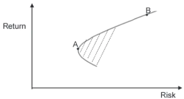
It is known that, with a set of risky assets, one can obtain portfolios that ill up a solid, lat and hyperbolic space (Merton, 1972, p. 1856), in a graphic of risk (measured by standard deviation) and return, as shown in Figure 1.
Figure 1. Portfolios formed from a set of risky assets
Considering that investors prefer more wealth to less wealth, and that they do not like risk (are risk averse) – both proposals on which various inance frameworks are based –, on can verify that various portfolio possibilities are dominated by better possibilities. One can think about dominance based on (i) risk (smaller risk for same return), (ii) return (greater return for same risk) or (iii) both (smaller risk and greater return). hus, in Figure 1, it can be observed that the portfolios in segment AB (and beyond B) are not dominated and, therefore, form the so-called eicient investment frontier.
a personal utility curve), the portfolio an investor chooses from the components of the eicient investment frontier is a matter to be resolved in the context of each individual investor. Investors with greater risk aversion prefer portfolios that are closer to the portfolio represented at point A, and investors with smaller risk aversion prefer portfolios closer to the one represented at point B (or beyond).
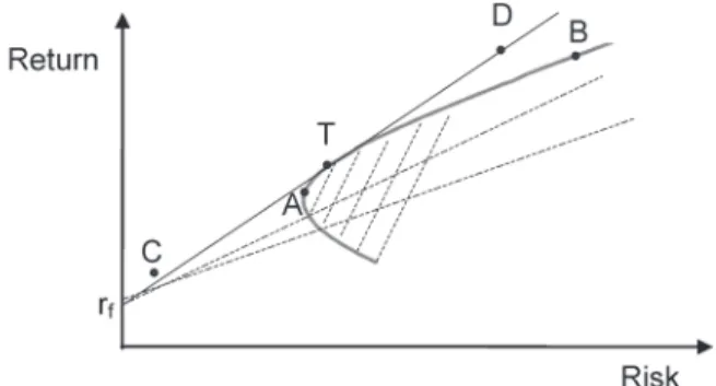
However, investors can buy a risk free asset (rf) as well as a set of risky assets (risky portfolio). In this case, portfolio possibilities (now with the risk free asset) expand to those shown in Figure 2 (Tobin, 1958). In this igure, it can be observed that the portfolios made up only of risky assets from segment AB in Figure 1 (the efficient investment frontier) are dominated by portfolios also made up of the risk free asset from line CD, called the capital market line (or CML).
Figure 2. Capital Market Line (line CD)
It can be seen, therefore, that the best risky asset portfolio for investors would be the portfolio T – the one that just touches the AB segment, regardless of investors’ risk aversion. Adequacy to the risk aversion of each individual investor would occur by allocating his money between risk free assets and the portfolio T. Investors with greater risk aversion prefer portfolios that are closer to the portfolio represented at point C (with greater allocation of their investments in the risk free asset – rf); investors with smaller risk aversion prefer portfolios that are closer to the portfolios represented at point F (with greater allocation of their investments in the portfolio T); and investors with a great appetite for risk can leverage their
investments in the portfolio T, approaching the portfolio represented in point D.
Please note that, if an investor chooses any other risky asset portfolio rather than the portfolio T, investment opportunities (according to the allocation between a risk free asset and a risky portfolio) would be comparatively worse than those obtained through the portfolio T, and the line including these possibilities would be less sloped than line CD (see Figure 3).
Figure 3. Portfolio possibilities with the Risk Free Asset
hus, the best portfolio for an investor would be the one with the greatest slope, measured according to Equation 3.
Eq. 3
In which, b = slope
Δy = variation of y Δx = variation of x
Using a portfolio C, with risk dpc and a return rc, and risk free asset with return rf and dp zero, one has Equation 4.
Eq. 4
In which, b = slope
rc = portfolio’s return
rf = risk free asset return (risk free rate)
his same slope is known as the Sharpe Ratio or IS (Sharpe, 1966).
In this context, one can conclude that a portfolio with a higher Sharpe Ratio (CIS+) is better than a portfolio with a smaller Sharpe Ratio (CIS-), since the former (CIS+) combined with the risk free asset would result in alternatives that would dominate the alternatives obtained from the second (CIS-) and the risk free asset.
There are several other portfolio performance measures, but the one used in this paper is the Sharpe Ratio, because the proposed portfolios were based on the establishment of the portfolio T – the latter being essentially the portfolio with the greatest IS, made up of risky assets.
2.2
Ibovespa
Ibovespa is the São Paulo Stock Exchange’s (BM&FBovespa) main index. Its goal is to be “the average performance index of the prices of the most traded and representative stocks in the Brazilian stock market” (BM&FBovespa, 2014a).
Ibovespa has always been criticized for the high concentration of certain shares in its composition, because its composition criteria is strongly based on liquidity and for having diferent criteria for maintaining and including shares (for example, Rabelo, 2007; Sheng & Saito, 2002; Takamatsu & Lamounier, 2006).
On September 11, 2014, BM&FBovespa announced Ibovespa’s new methodology. his change took place partially in January 2014, and fully, in May 2014.
The changes impact the rules (i) for inclusion in the index (increase in the negotiability index, change in the criteria for participating in trading sessions, and not being “penny stock” or being listed as a “special situation”); and (ii) the deinition of weight of each share in the index (which gives greater importance to the total traded value and establishes a participation limit).
It is not the purpose of this paper to assess whether the changes made to Ibovespa solve the criticism addressed to it.
2.3
A brief review of the literature on
portfolio optimization
Nothing guarantees that market indexes (for example, Ibovespa) are eicient portfolios (homé, Leal & Almeida, 2011). Several authors have dedicated themselves to checking whether portfolios that are optimized by certain rules (for example, the modern portfolio theory) are capable of being superior to market indexes. Moreover, according to common sense, market indexes are often far from the eicient investment frontier (Levy & Roll, 2010).
Hieda and Oda (1998) studied twelve four-month periods between 1994 and 1998. They set up three investment strategies: (1) Ibovespa (Old), (2) portfolio T (considering CDI as the risk free asset and ofering the 20 most traded shares to make up this portfolio, using quarterly parameters) and (3) the portfolio that they called the naïve strategy (with the same weight for each of the 20 most liquid shares). he analyzed portfolio T only reached a higher Sharpe Ratio in one of the twelve four-month periods.
Bruni and Fama (1998) analyzed the efects of diversiication, in the period between July 1993 and June 1998, with the 20 most liquid stocks. he authors studied (1) the naïve strategy (same weight) and (2) a risk and return optimization strategy, based on the modern portfolio theory, for various sliding windows (12, 24 and 36 months). he authors concluded that all the strategies resulted in better returns when compared to Ibovespa. hese results were maintained when analyzing the Sharpe Ratios of the various strategies and Ibovespa. he strategy with a moving average of 12 months proved to be the best one.
third party funds, questioning the eiciency of the analyzed indexes. However, they highlighted that macroeconomic instability and high interest rates may have contributed to the ineiciency of the indexes.
DeMiguel, Garleppi, & Uppal (2009) tested the naïve strategy for US market data, comparing it to 14 different optimization models, indicating the superiority of the former when compared to the others; the indings were obtained through the Sharpe Ratio and the certainty equivalent return. he choice for the naïve strategy is based on (i) the ease of operation (due to non-dependence of estimating the future based on historical parameters such as return and risk), and (ii) the use of this approach by investors. he authors indicate that the naïve strategy is more likely to produce better results the higher the number of assets involved – by leveraging the power of diversiication. Empirical tests involved scenarios for 3, 9, 11, 21 and 24 assets.
Defying common sense, Levy and Roll (2010) used reverse engineering to indicate that small variations in mean and variance parameters within estimation errors may indicate that market indexes are eicient from the mean-variance point of view.
Thomé et al. (2011) tested minimum variance portfolios. The authors constructed portfolios with maximum participation limits for each share ranging from 10% to 100% (that is, with no limits). he portfolio with no weight limits was not superior to Ibovespa, but the portfolio with maximum weight of 10% was superior to Ibovespa. he latter portfolio, however, was not superior to a portfolio formed by the naïve strategy (equally weighted) and was surpassed by actively managed funds. he maximum 10% weight limit, according to the authors, ensured greater stability and composition uniformity of the portfolio at every quarter. he authors analyzed the period between April 1998 and December 2008.
Studying 677 daily obser vations concerning 45 assets between March 2009 and November 2011, Santos and Tessari (2012)
compared the performance of Ibovespa to that of the naïve strategy and other optimization strategies. he results indicate that (a) the mean-variance strategy presented the best results in terms of return, followed by the minimum variance, naïve and Ibovespa strategies, and (b) the mean-variance and minimum variance strategies presented smaller standard deviations than the other two strategies (naïve and Ibovespa). he Sharpe Ratios of the mean-variance and minimum variance strategies are greater than those of the naïve and Ibovespa strategies. he authors point out that any diferences in maximum asset allocation restrictions (being more flexible), analysis period, used algorithm and others can explain the diferent results previously presented by other authors.
Analyzing shares that made up Ibovespa between January 1998 and December 2011, Santiago and Leal (2015) formed portfolios based on the naïve strategy (from 6 to 16 assets per portfolio) and on minimum variance (with maximum weight of 10%). he selection criterion, among the possible shares, was the greatest Sharpe Ratio. he naïve portfolios did not surpass Ibovespa or the minimum variance portfolio. he authors also compared the naïve portfolio to the Investment Shares Funds (Fundos de Investimento em Ações, FIA), concluding that the naïve portfolio was equivalent to the latter.
This paper tests a period made up of 34 quarters, and ofers 118 shares for portfolio formation. Other studies do not match these numbers. It is also the irst known study to test New Ibovespa.
3
Methodology
3.1
Sample
mentioned portfolios. he returns of the Old Ibovespa and of New Ibovespa were also obtained from BM&FBovespa (2014b).
he prices (adjusted for corporate events) of all the shares that made up these 34 portfolios (118 shares) were obtained from the Economática®
information system (for the period between August 30, 2002 and May 2, 2014).
he historical series of the daily Selic rate were obtained from Brazil’s Central Bank’s (Banco Central do Brasil) time series system (also for the period between August 30, 2002 and May 2, 2014).
3.2
Formation of portfolios T
he portfolio T was obtained with only Brazilian assets (shares traded in Bovespa and a risk free asset – considered as the Selic) and without allowing leverage (the possibility of short selling was discarded).
For each of the 34 (four-month) periods analyzed, the portfolio with shares that had the greatest Sharpe Ratio was calculated (portfolio T), ofering for its composition the shares that made up Ibovespa (according to the new methodology) in the respective period (four months). Weekly returns were used for a four-month history (the four months previous to the efectiveness of the portfolio). Portfolio T was achieved by routines developed by the authors and carried out in Microsoft Excel®.
Some shares that made up Ibovespa in at least one of the 34 periods analyzed are no longer traded, but their historical price series are still made available by Economática. Other shares changed their names, for several reasons. In this paper, the name changes presented in Table 1 were considered.
Table 1
Changes in the names of certain shares
Original name Current name Original name Current name
BMEF3 BVMF3 LLXL3 PRML3
BRTO4 OIBR4 PCAR5 PCAR4
CLSC6 CLSC4 PRGA3 BRFS3
CESP4 CESP5 VCPA3 FIBR3
ECOD3 VAGR3 TLPP4 VIVT4
ELPL6 ELPL4 TSPP4 VIVO4
ITAU4 ITUB4 TCSL3 TIMP3
he composition of portfolio T, for each of the 34 analyzed four-month periods, is presented in Appendix A.
3.3
Hypotheses and statistical approach
he goal of this paper was to determine whether Ibovespa, Old and New, would be the best alternative for investors, considering investment possibilities (risky and risk free) in the Brazilian market.
Therefore, it is necessary to test the diference in return and the diference in variance between pairs of portfolio ((I) portfolio T versus New Ibovespa, (II) portfolio T versus Old
Ibovespa, and (III) New Ibovespa versus Old Ibovespa), plus the diference in the relationship between return and variance measured by the Sharpe Ratio (IS).
I – Pair of portfolios — portfolio T versus New Ibovespa:
HI-I0: mean of portfolio T = mean of New Ibovespa
HI-Ia: mean of portfolio T ≥ mean of New Ibovespa
HI-II0: variance of portfolio T = variance of New Ibovespa
HI-IIa: variance of portfolio T ≠ variance of New Ibovespa
HI-III0: IS of portfolio T = IS of New Ibovespa
HI-IIIa: IS of portfolio T ≥ IS of New Ibovespa
II – Pair of portfolios — portfolio T versus Old Ibovespa:
HII-I0: mean of portfolio T = mean of Old Ibovespa
HII-Ia: mean of portfolio T ≥ mean of Old Ibovespa
HII-II0: variance of portfolio T = variance of Old Ibovespa
HII-IIa: variance of portfolio T ≠ variance of Old Ibovespa
HII-III0: IS of portfolio T = IS of Old Ibovespa
HII-IIIa: IS of portfolio T ≥ IS of Old Ibovespa
III – Pair of portfolios — New Ibovespa versus Old Ibovespa:
HIII-I0: mean of New Ibovespa = mean of Old Ibovespa
HIII-Ia: mean of New Ibovespa ≥ mean of Old Ibovespa
HIII-II0: variance of New Ibovespa = variance of Old Ibovespa
HIII-IIa: variance of New Ibovespa ≠ variance of Old Ibovespa
HIII-III0: IS of New Ibovespa = IS of Old Ibovespa
HIII-IIIa: IS of New Ibovespa ≥ IS of Old Ibovespa
For the mean test, the paired data variant was used, since both portfolios being compared are present on the same dates. Levine, Stephan, Krehbiel and Berenson (2012) indicate the use of paired tests for two interrelated populations. Lapponi (2000) emphasizes that, in these cases, the variable of interest is the diference between both pairs of samples rather than the samples themselves (since they are paired, both samples are of the same size). In this paper, the focus is on the historical series of the daily diference in the return of the portfolios, and not on the individual values themselves, which, according to Levine et al. (2012), also indicates the interrelated or paired population test. Costa (1977) indicates that reducing the sample to a single one made up of the diferences increases the power of explanation of the test, when compared with unpaired samples: “whenever possible and justifiable, we should pair the data, because in this way we shall have an additional information that will lead us to statistically stronger results” (Costa, 1977, p. 109).
If the return distributions are normal distributions, the equality of the mean will be tested using the one-tailed t-test for paired data. If the return distributions are not normal distributions, the equality of the mean will be tested using the nonparametric Wilcoxon test for paired data, which, for one-tailed consideration, will be assumed as a symmetrical distribution. According to Fávero, Beliore, Silva and Chan (2009), the Wilcoxon test is recommended to test the mean diference of two paired samples, and according to Maroco (2007) this test is used to compare two population means from paired data, replacing the t-test. Santiago and Leal (2015) and homé et al. (2011) used the Wilcoxon test.
The normality of the distributions is tested using the Kolmogorov-Smirnov (KS) test, in which the null hypothesis is that distribution is normal and the alternative hypothesis is that distribution is not normal.
4
Data Analysis
It can be observed that the portfolios T formed for each of the four-month periods present a reduced number of shares compared to
the number of shares present in New Ibovespa and, consequently, shares with great weight in the portfolio. It can also be observed that there is, every four months, a major change in the composition of the portfolio T (Table 2). he change in portfolio composition is credited by some authors, such as Jagannathan and Ma (2003), to errors in the estimation of historical returns. Jagannathan and Ma (2003) suggest the minimum variance portfolio strategy as an alternative to stabilize weights.
Table 2
Composition of Portfolio T x Composition of New Ibovespa
Portfolio T New Ibovespa
Quarter Amount of Shares
% Repeated Shares from t-1
Greater Weight
Share
Weight 3 Greater
Shares
Amount of Shares
% Repeated Shares from t-1
Greater Weight
Share
Weight 3 Greater
Shares
1 7 48.4% 79.7% 41 18.4% 33.6%
2 6 33.3% 34.7% 74.4% 39 100.0% 14.3% 30.6%
3 7 42.9% 26.7% 78.5% 37 100.0% 14.6% 32.6%
4 8 25.0% 20.8% 58.1% 39 94.9% 14.5% 28.9%
5 2 0.0% 62.2% 100.0% 40 97.5% 15.0% 30.7%
6 5 20.0% 41.7% 91.3% 42 95.2% 14.5% 30.8%
7 7 14.3% 23.7% 61.2% 44 95.5% 14.5% 31.4%
8 3 33.3% 49.8% 100.0% 47 93.6% 14.7% 32.6%
9 7 0.0% 56.3% 81.4% 48 95.8% 15.8% 35.6%
10 8 25.0% 42.3% 76.3% 49 93.9% 15.8% 35.6%
11 7 14.3% 30.0% 77.9% 51 90.2% 15.7% 33.9%
12 7 28.6% 35.9% 80.2% 51 90.2% 15.4% 33.1%
13 8 12.5% 26.7% 67.6% 54 90.7% 14.8% 32.8%
14 6 16.7% 24.8% 61.0% 57 94.7% 12.7% 31.8%
15 8 0.0% 47.4% 85.2% 61 90.2% 15.7% 35.5%
16 5 60.0% 39.2% 81.5% 66 92.4% 15.5% 36.2%
17 6 0.0% 36.3% 77.1% 66 97.0% 14.7% 33.3%
18 5 20.0% 45.4% 96.6% 68 85.3% 14.4% 32.7%
19 1 100.0% 100.0% 100.0% 55 100.0% 14.0% 32.4%
20 8 12.5% 56.3% 86.6% 52 96.2% 13.7% 35.7%
21 12 16.7% 28.3% 55.7% 51 98.0% 13.3% 34.5%
22 6 16.7% 30.0% 73.7% 54 90.7% 13.4% 33.1%
23 7 0.0% 36.4% 77.3% 57 93.0% 12.9% 32.3%
24 8 12.5% 44.4% 78.3% 58 96.6% 10.6% 29.3%
25 8 25.0% 29.5% 68.8% 58 96.6% 12.8% 31.9%
26 10 30.0% 22.6% 63.2% 60 95.0% 12.2% 31.0%
27 7 42.9% 32.6% 67.0% 63 92.1% 10.7% 29.4%
28 8 25.0% 37.8% 85.0% 62 100.0% 11.1% 29.7%
29 12 41.7% 28.0% 57.0% 65 92.3% 10.1% 27.0%
30 5 20.0% 36.7% 87.2% 64 98.4% 10.8% 27.7%
31 13 7.7% 34.6% 60.0% 66 97.0% 9.4% 26.9%
32 10 20.0% 25.1% 60.0% 69 95.7% 9.6% 25.8%
33 8 0.0% 26.2% 70.0% 73 93.2% 8.3% 23.4%
Comparative analysis of the return and risk of the portfolio T in New Ibovespa and Old Ibovespa will be divided into two parts: (i) the entire period (composed of the 34 four-month periods) and (ii) the individual periods (composed of each four-month period individually).
4.1
Entire period
Altogether, 2.805 daily returns over 34 four-month periods were analyzed. All portfolios traded in over 99.8% of the days. he Kolmogorov-Smirnov test rejected the normality of return distributions for the entire period for the portfolio T (p-value of 0.000), for New Ibovespa (p-value 0.000) and for Old Ibovespa (p-value of 0.000).
The average daily return in the entire period (January 1, 2003 to April 30, 2014) (i) for the portfolio T was 0.111% p.d. (ii) for New Ibovespa was 0.079% p.d. and (iii) for Old Ibovespa was 0.070% p.d. The average daily return of the portfolio T is statistically superior to New Ibovespa (p-value of the nonparametric test, for one-tailed paired data – assuming symmetrical distribution, is 0.063), and also to Old Ibovespa (p-value of the nonparametric test, for one-tailed paired data – assuming symmetrical distribution, is 0.012). he average daily return of New Ibovespa is statistically superior to Old Ibovespa (p-value of the nonparametric test for one-tailed paired data – assuming symmetrical distribution, is 0.078).
he standard deviation of daily returns throughout the period (i) for the portfolio T was 1.61%, (ii) for New Ibovespa was 1.74%, and (iii) for Old Ibovespa was 1.79%. he standard deviation of daily returns of the portfolio T is statistically diferent from the standard deviation of daily returns of New Ibovespa (p-value of the Levene test is 0.001) and also from Old Ibovespa (p-value of the Levene test is 0.000). he standard
deviation of New Ibovespa daily returns is statistically diferent from the standard deviation of daily returns of Old Ibovespa (p-value of the Levene test is 0.071).
The results indicate that the portfolio T dominates New Ibovespa and Old Ibovespa (it presents greater return and smaller standard deviation). herefore, Ibovespa (New or Old) would not be part of the set of eicient portfolios (ex post). here are also indications that New Ibovespa dominates Old Ibovespa (greater return and smaller standard deviation).
Regarding excess return (return above risk free asset rate), the results are the same (even considering that the risk free asset rate was variable over time). he average daily return of the risk free asset, throughout the period, is 0.049% p.d..
The Sharpe ratio was not statistically tested, because the daily IS was not calculated (its calculation requires standard deviation). However, with the above indications, it can be said that the Sharpe Ratio of the portfolio T (0.0389) is greater than New Ibovespa (0.0173) and Old Ibovespa (0.0117). he same could be said about the superiority, measured by the Sharpe Ratio, of New Ibovespa compared to Old Ibovespa.
hus, considering the entire period, the portfolio T would have been a better investment alternative. he research hypotheses listed in item 3.3, for the entire period, were answered with the tests above mentioned.
4.2
Individual periods
Table 3
Normality Test (p-value of the Kolmogorov-Smirnov Test)
Quarter Portfolio T New Ibovespa Old Ibovespa Quarter Portfolio T New Ibovespa Old Ibovespa
1 0.880 0.924 0.946 18 0.235 0.553 0.618
2 0.783 0.951 0.854 19 0.507 0.759 0.677
3 0.998 0.875 0.887 20 0.955 0.274 0.496
4 0.871 0.997 0.992 21 0.753 0.343 0.377
5 0.914 0.812 0.925 22 0.659 0.412 0.346
6 0.965 0.933 0.726 23 0.863 0.982 0.988
7 0.698 0.292 0.442 24 0.864 0.524 0.985
8 0.656 0.766 0.628 25 0.498 0.479 0.639
9 0.488 0.572 0.635 26 0.520 0.303 0.304
10 0.768 0.836 0.820 27 0.510 0.969 0.999
11 0.804 0.638 0.449 28 0.894 0.485 0.626
12 0.909 0.889 0.723 29 0.263 0.782 0.978
13 0.194 0.879 0.658 30 0.814 0.995 0.924
14 0.219 0.483 0.497 31 0.830 0.934 0.967
15 0.939 0.566 0.723 32 0.632 0.770 0.600
16 0.410 0.572 0.566 33 0.867 0.944 0.988
17 0.924 0.986 0.979 34 0.915 0.532 0.777
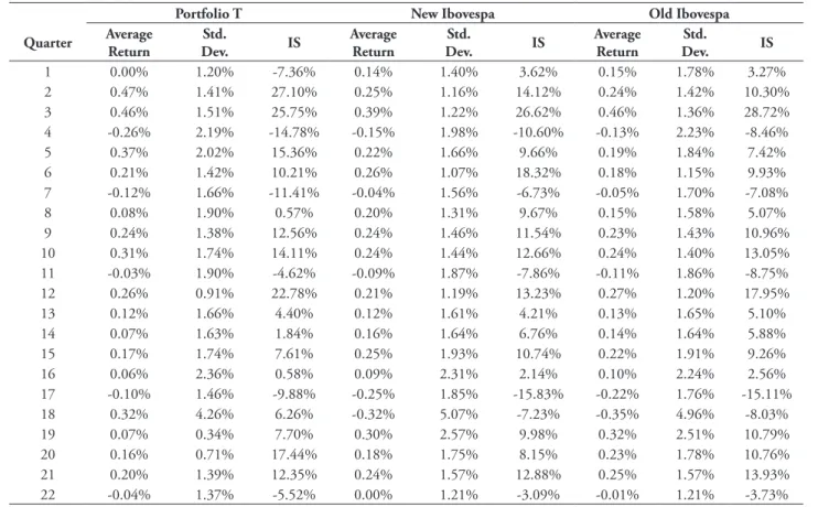
Table 4 presents, on a daily basis, the average return, the standard deviation and the Sharpe Ratio for each four-month period (1-34) and for (i) the portfolio T, (ii) New Ibovespa, and (iii) Old Ibovespa.
Table 4
Daily Average Return, Standard Deviation and Sharpe Ratio (IS) for each one of the 34 four-month periods analyzed for (i) portfolio T, (ii) New Ibovespa and (iii) Old Ibovespa
Portfolio T New Ibovespa Old Ibovespa
Quarter Average Return
Std.
Dev. IS
Average Return
Std.
Dev. IS
Average Return
Std.
Dev. IS
1 0.00% 1.20% -7.36% 0.14% 1.40% 3.62% 0.15% 1.78% 3.27%
2 0.47% 1.41% 27.10% 0.25% 1.16% 14.12% 0.24% 1.42% 10.30%
3 0.46% 1.51% 25.75% 0.39% 1.22% 26.62% 0.46% 1.36% 28.72%
4 -0.26% 2.19% -14.78% -0.15% 1.98% -10.60% -0.13% 2.23% -8.46%
5 0.37% 2.02% 15.36% 0.22% 1.66% 9.66% 0.19% 1.84% 7.42%
6 0.21% 1.42% 10.21% 0.26% 1.07% 18.32% 0.18% 1.15% 9.93%
7 -0.12% 1.66% -11.41% -0.04% 1.56% -6.73% -0.05% 1.70% -7.08%
8 0.08% 1.90% 0.57% 0.20% 1.31% 9.67% 0.15% 1.58% 5.07%
9 0.24% 1.38% 12.56% 0.24% 1.46% 11.54% 0.23% 1.43% 10.96%
10 0.31% 1.74% 14.11% 0.24% 1.44% 12.66% 0.24% 1.40% 13.05%
11 -0.03% 1.90% -4.62% -0.09% 1.87% -7.86% -0.11% 1.86% -8.75%
12 0.26% 0.91% 22.78% 0.21% 1.19% 13.23% 0.27% 1.20% 17.95%
13 0.12% 1.66% 4.40% 0.12% 1.61% 4.21% 0.13% 1.65% 5.10%
14 0.07% 1.63% 1.84% 0.16% 1.64% 6.76% 0.14% 1.64% 5.88%
15 0.17% 1.74% 7.61% 0.25% 1.93% 10.74% 0.22% 1.91% 9.26%
16 0.06% 2.36% 0.58% 0.09% 2.31% 2.14% 0.10% 2.24% 2.56%
17 -0.10% 1.46% -9.88% -0.25% 1.85% -15.83% -0.22% 1.76% -15.11% 18 0.32% 4.26% 6.26% -0.32% 5.07% -7.23% -0.35% 4.96% -8.03%
19 0.07% 0.34% 7.70% 0.30% 2.57% 9.98% 0.32% 2.51% 10.79%
20 0.16% 0.71% 17.44% 0.18% 1.75% 8.15% 0.23% 1.78% 10.76%
21 0.20% 1.39% 12.35% 0.24% 1.57% 12.88% 0.25% 1.57% 13.93%
Portfolio T New Ibovespa Old Ibovespa
Quarter Average Return
Std.
Dev. IS
Average Return
Std.
Dev. IS
Average Return
Std.
Dev. IS
23 0.20% 1.54% 10.32% -0.04% 1.52% -5.35% -0.03% 1.53% -4.51%
24 0.08% 0.90% 4.54% 0.17% 1.28% 9.85% 0.08% 1.07% 3.82%
25 0.13% 1.07% 8.19% -0.04% 1.04% -8.39% -0.05% 1.05% -9.15% 26 -0.01% 1.51% -3.95% -0.15% 1.63% -11.93% -0.17% 1.73% -12.19%
27 0.11% 1.30% 5.31% 0.06% 1.60% 1.23% 0.02% 1.77% -1.25%
28 0.14% 0.75% 13.76% 0.09% 1.11% 4.92% 0.11% 1.17% 6.24%
29 -0.08% 1.13% -9.65% -0.06% 1.46% -6.39% -0.08% 1.66% -6.68%
30 0.08% 0.94% 5.95% 0.10% 1.05% 6.76% 0.09% 1.17% 5.43%
31 0.00% 1.08% -2.98% -0.02% 1.09% -4.08% -0.10% 1.16% -11.01% 32 -0.04% 1.04% -6.36% -0.10% 1.25% -10.54% -0.12% 1.47% -10.23%
33 0.20% 1.13% 14.49% 0.08% 1.00% 4.42% 0.04% 1.23% 0.64%
34 -0.04% 1.25% -6.72% 0.02% 1.25% -1.77% 0.01% 1.30% -2.65%
Comparing the return of the portfolio T to New Ibovespa in each of the four-month periods, through the one-tailed t-test for paired data, it can be said that the return of the portfolio T was statistically superior to that of New Ibovespa in ive four-month periods (14.7% of the cases): 2 (p-value 0.048), 18 (0.051), 23 (0.035), 25 (0.056) and 26 (0.086). The return of New Ibovespa did not statistically surpass the return of the portfolio T in any of the four-month periods.
Comparing the standard deviation of the portfolio T with the standard deviation of New Ibovespa in each of the four-month periods, through the F-test, it can be said that (i) the standard deviation of the portfolio T was statistically smaller than that of New Ibovespa in nine four-month periods (26.5% of cases), 12 (p-value 0.020), 17 (0.029), 19 (0.000), 20 (0.000), 24 (0.002), 27 (0.058), 28 (0.001), 29 (0.020), and 32 (0.092) and (ii) the standard deviation of the portfolio T was statistically greater than that of New Ibovespa in six four-month periods (17.6% of cases): 2 (p-value 0.076), 3 (0.054), 5 (0.071), 6 (0.011), 8 (0.001), and 10 (0.091). he lower number of shares in the portfolio T when compared to New Ibovespa, which could restrict the diversiication capacity of the portfolio T, did not hinder the performance, in terms of risk, of the portfolio T when compared to New Ibovespa.
he portfolio T dominated New Ibovespa in thirteen four-month periods. hose in which
(i) the return of the portfolio T was statistically greater than that of New Ibovespa and the standard deviation was statistically smaller or equal (four-month periods 18, 23, 25 and 26) or (ii) the standard deviation of the portfolio T was statistically smaller than that of New Ibovespa and the return was statistically equal (12, 17, 19, 20, 24, 27, 28, 29 and 32). New Ibovespa dominated the portfolio T in ive four-month periods: 3, 5, 6, 8 and 10 (smaller risk and equal return). In terms of dominance, the portfolio T dominated New Ibovespa in 72.2% of cases in which there was dominance (13 in 18).
he details are not displayed, such as for comparison between the portfolio T and New Ibovespa, but the portfolio T dominated Old Ibovespa in ifteen of the eighteen four-month periods in which there was dominance (83.3% of cases). New Ibovespa dominated Old Ibovespa in seven of the nine cases in which there was dominance (77.8% of cases).
Kolmogorov-Smirnov test is 0.945), for New Ibovespa (p-value 0.871) and for Old Ibovespa (p-value 0.842). he average Sharpe Ratio for the portfolio T is statistically greater than that of New Ibovespa (p-value of the tailed t-test for paired data is 0.067) and is also statistically superior to Old Ibovespa (p-value 0.014). he average Sharpe Ratio of New Ibovespa is statistically greater than that of Old Ibovespa (p-value 0.036). In 52.9% (18 of 34) of the four-month periods, the Sharpe Ratio of the portfolio T was greater than that of New Ibovespa. In 58.5% (20 of 34) of the four-month periods, the Sharpe Ratio of the portfolio T was greater than that of Old Ibovespa. In 61.8% (21 of 37) of the four-month periods, the Sharpe Ratio of New Ibovespa was higher than that of Old Ibovespa.
Considering only the four-month period with a positive Sharpe Ratio (19 four-month periods), the average Sharpe Ratio was 0.115 for the portfolio T, 0.103 for New Ibovespa, and 0.094 for Old Ibovespa. he distribution of the 19 positive Sharpe Ratios is normal for the portfolio T (p-value of the Kolmogorov-Smirnov test is 0.983), for New Ibovespa (p-value 0.814) and for Old Ibovespa (p-value 0.502). he average Sharpe Ratio for the portfolio T is not statistically greater than that of New Ibovespa (p-value of the tailed t-test for paired data is 0.218) and is, however, statistically greater than that of Old Ibovespa (p-value 0.065). he average Sharpe Ratio of New Ibovespa is statistically greater than that of Old Ibovespa (p-value 0.098). In 47.4% (9 of 19) of the four-month periods, the Sharpe Ratio of the portfolio T was greater than that of New Ibovespa. In 57.9% (11 of 19) of the four-month periods, the Sharpe Ratio of the portfolio T was greater than that of Old Ibovespa. In 52.6% (10 of 19) of the four-month periods, the Sharpe Ratio of New Ibovespa was greater than that of Old Ibovespa.
4.3
Robustness
he robustness analysis focused on the comparison, for the entire period, between the portfolio T and New Ibovespa. One can imagine that the four-month periods in which
the portfolio T consists of only a few assets is capable of distorting the results presented herein, favoring the portfolio T over New Ibovespa. It is noteworthy that the portfolios were set up with the history of the four-month period previous to their efectiveness, and, therefore, it would have been necessary that these few assets would have had favorable results over two consecutive four-month periods – the portfolio’s estimation four-month period and the portfolio’s four-month period of its efectiveness.
It can also be observed that the small number of assets in the portfolio T could impair its ability to diversify. On the one hand, since Evans and Archer (1968), it has been show that it is not necessary a large number of assets to largely capture the efects of diversiication (in Brazil, see, for example, Oliveira & Paula, 2008). On the other hand, Chance Shynkevich and Yang (2011) disagree in general terms about this standard line of thought, recommending a greater amount of shares. Studies related to the speciic topic of this paper indicate the superiority of portfolios formed by a larger number of assets (DeMiguel et al., 2009; homé et al., 2011).
The amount of assets per portfolio T varies from 1 to 13 assets over the 34 four-month periods analyzed. here is a portfolio T with only
one asset, and also one portfolio T with thirteen assets. Table 5 presents the number of portfolios T for each amount of assets.
Table 5
Amount of assets per portfolio and number of portfolios (absolute and relative)
Amount of Assets Number of Portfolios T Proportion of Total Portfolios T
1 1 2.9%
2 1 2.9%
3 1 2.9%
4 0 0.0%
5 4 11.8%
6 4 11.8%
7 8 23.5%
8 9 26.5%
9 0 0.0%
10 2 5.9%
11 1 2.9%
12 2 5.9%
13 1 2.9%
Total 34 100%
It can be observed in Table 5 that 20.6% of the portfolios T have ive assets or less. Table 6 presents the average returns of the portfolio T and of the New Ibovespa portfolio, the standard deviation of the portfolio T and the New Ibovespa portfolio, the p-value of mean equality test, and the p-value of the variance equality test, if the portfolios with up to a certain number of assets (ranging from 1 to 5) were eliminated from the
sample of the entire period. Normality of return was tested for each exclusion scenario. he p-value of the Kolmogorov-Smirnov test indicates that the distributions in Table 6 are not normal (p test value for the distributions of both portfolios with the exclusion of one to four assets is 0.000, and, for the exclusion of ive assets, the p-value of the distribution of the portfolio T is 0.002 and of New Ibovespa is 0.014).
Table 6
Portfolio T Performance Versus New Ibovespa Performance if Periods in which the Portfolio T had a Number of Assets that was Equal to or Smaller than a Certain Number of Assets were Eliminated (from 1 to 5 Assets)
Portfolio T New Ibovespa Equality Test
Amount of
Assets Return
Standard
Deviation Return
Standard Deviation
Mean (p-value)
Variance (p-value)
0 0.111% 1.61% 0.079% 1.74% 0.063 0.001
1 0.113% 1.63% 0.073% 1.71% 0.050 0.078
2 0.104% 1.61% 0.068% 1.71% 0.063 0.042
3 0.105% 1.60% 0.063% 1.73% 0.067 0.013
4 0.105% 1.60% 0.063% 1.73% 0.067 0.013
It can be observed that, even excluding the four-month periods in which the portfolio T was comprised of less than ive assets, the portfolio T would have been superior to New Ibovespa in return (greater) and risk (smaller). For scenarios in which the portfolios T with over ive assets (6 to 12, successively) are excluded, the average equality tests indicate that (i) the return of the portfolio T was equal to the return of the New Ibovespa portfolio, and (ii) that the variance of the portfolio T was smaller than the variance of New Ibovespa. hus, the portfolio T would have been better than New Ibovespa in all exclusion scenarios.
Additionally, analyses with no extreme values were carried out. Two separate scenarios were analyzed:
In the irst one, values above and below 3.09 standard deviations were eliminated. If the distribution was normal, it would be equivalent to eliminate 0.2% of the observations (0.1% on each side, assuming normal distribution). In total, for the portfolio T, 36 observations were eliminated (1.28% of the 2.805 values), and 35 observations of New Ibovespa (1.25% of the 2.805 values). Observations fell to 2.752, distributions continued to be not normal (p-value of the KS test was 0.001 and 0.014 for portfolio T and New Ibovespa, respectively). he average return of the portfolio T was 0.1064% and of New Ibovespa was 0.0684%, portfolio T being statistically higher (p-value of the non-parametric test 0.065). he standard deviation of the portfolio T was 1.39% and of New Ibovespa was 1.47%, portfolio T being statistically better (p-value of the non-parametric test 0.001).
In the second scenario, the values above and below 2.58 standard deviations (equivalent to 1.0% of observations, if distributions were normal) were eliminated. In all, 63 observations (2.25%) of the portfolio T and 61 observations (2.17%) of New Ibovespa were eliminated, with 2.711 observations remaining. he portfolio T was statistically superior to New Ibovespa in terms of average return (0.1085% versus 0.0750%, with p-value of the non-parametric test equal to 0.053), and in terms of standard deviation (1.33% versus
1.40%, p-value of the non-parametric test equal to 0.001).
hese analyses with elimination of extreme values continue to indicate the superiority of the portfolio T when compared to New Ibovespa.
5
Final Considerations
Modern portfolio theory says that there is a risky assets’ portfolio that all investors should have – the portfolio T. he portfolio T would be one of the portfolios in the eicient investment frontier. The other portfolios in the efficient investment frontier, even not being dominated by any other risky asset portfolio, would not be the best alternative for investors.
Is Ibovespa this portfolio T? Is there a portfolio that would be better for investor? Is there a portfolio that would dominate Ibovespa?
hirty four four-month periods (from January 1, 2003 to April 30, 2014) were studied, analyzing Old Ibovespa, New Ibovespa and the portfolio T (the latter calculated from modern portfolio theory, considering the Selic as the risk free asset).
For the entire period, the portfolio T presented statistically greater returns and smaller standard deviations than New Ibovespa and Old Ibovespa, and is thus a better alternative for investors. New Ibovespa and Old Ibovespa were dominated by the portfolio T (ex post). he portfolio T’s Sharpe Ratio was also higher than New Ibovespa and Old Ibovespa. New Ibovespa, in turn, dominated Old Ibovespa (greater return and smaller risk).
In accepting the assumptions made in this study, New Ibovespa or Old Ibovespa are not the best investment alternatives.
ive of the eighteen cases. When all 34 four-month periods are considered, the average Sharpe Ratio for the portfolio T was statistically greater than the average Sharpe Ratio for New Ibovespa, and is individually greater in 52.9% of cases. When only the four-month periods in which the Sharpe Ratio was positive are considered, there was no statistical superiority in either of the two portfolios (portfolio T and New Ibovespa), and in 47.4% of the four-month periods the Sharpe Ratio of the portfolio T surpassed New Ibovespa.
he limitations of the portfolio T are as follows: (i) few number of component shares, (ii) consequent large weight of individual shares in the portfolio, and (iii) major change in the composition of the same (see Table 2).
he limitations of this paper are in the definition of the assumption (including the choice of the risk free asset), in the alternatives used for historical data and periodicity, and in the assumption that future expectations are well represented by the historical data obtained over the estimation period.
References
BM&FBOVESPA. (2014a). O q u e é o Ib o v e s p a ? Re c u p e r a d o d e h t t p : / / w w w. bmfbovespa.com.br/indices/ResumoIndice. aspx?Indice=Ibovespa&idioma=pt-br
BM&FBOVESPA. (2014b). Série retroativa do Ibovespa com base na metodologia adotada em Setembro de 2013. Recuperado de http://www. bmfbovespa.com.br/Indices/download/SERIE- RETROATIVA-DO-IBOV-METODOLOGIA-VALIDA-A-PARTIR-09-2013.pdf
Bruni, A. L., & Famá, R. (1998). Moderna teoria de portfólios: É possível captar, na prática, os benefícios decorrentes de sua utilização? Resenha da BM&F, (128), 19-34.
Chance, D. M., Shynkevich, A., & Yang, T. (2011). Experimental evidence on portfolio size and diversiication: Human biases in naive security selection and portfolio construction. Financial Review, 46(3), 427-457.
Copeland, T., Weston, J. F., & Shastri, K. (2005). Financial theory and corporate policy (4th ed.). Boston: Pearson.
Costa, P. L. O., Neto. (1977). Estatística. São Paulo: Edgard Blücher.
DeMiguel, V., Garlappi, L., & Uppal, R. (2009). Optimal versus naive diversification: How ineicient is the 1/n portfolio strategy? he Review of Financial Studies, 22(5), 1915-1953.
Elton, E. J., Gruber, M. J., Brown, S. J., & Goetzmann, W. N. (2004). Moderna teoria de carteiras e análise de investimentos. São Paulo: Atlas.
Evans, J. L., & Archer, S. H. (1968). Diversiication and the reduction of dispersion: An empirical analysis. Journal of Finance, 23(5), 761-767.
Fávero, L. P., Beliore, P., Silva, F. L., & Chan, B. L. (2009). Análise de dados: Modelagem multivariada para tomada de decisões. Rio de Janeiro: Elsevier.
Hagler, C. E. M., & Brito, R. D. O. (2007). Sobre a eiciência dos índices de ações brasileiros. Revista de Administração, 42(1), 74-85.
Hieda, A., & Oda, A. L. (1998). Um estudo sobre a utilização de dados históricos no modelo de Markowitz aplicado à bolsa de valores de São Paulo. Seminários em Administração, São Paulo, SP, Brasil, 9. Recuperado de http://www.semead. com.br/edicoes-anteriores-2/
Jagannathan, R., & Ma, T. (2003). Risk reduction in large portfolios: Why imposing the wrong constraints helps. Journal of Finance, 58(4), 1651-1684.
Lapponi, J. C. (2000). Estatística usando Excel. São Paulo: Lapponi Treinamento e Editora.
Levy, M., & Roll, R. (2010). he market portfolio may be mean/variance efficient after all. The Review of Financial Studies, 23(6), 2464-2491.
Markowitz, H. M. (1952). Portfolio Selection. Journal of Finance, 7(1), 77-91.
Maroco, J. (2007). Análise estatística com utilização do SPSS (3a ed.). Lisboa: Edições Sílabo.
Merton, R. C. (1972). An analytic derivation of the eicient portfolio frontier. he Journal of Financial and Quantitative Analysis, 7(4), 1851-1872.
Oliveira, F. N., & Paula, E. L. (2008). Determinando o grau ótimo de diversiicação para investidores usuários de home brokers. Revista Brasileira de Finanças, 6(3), 437-461.
Rabelo, S. S. T. (2007). Performance das melhores práticas de governança corporativa: Um estudo de carteiras (Dissertação de Mestrado em Administração). Universidade Federal de Uberlândia, Uberlândia, Brasil.
Santiago, D. C., & Leal, R. P. C. (2015). Carteiras igualmente ponderadas com poucas ações e o
pequeno investidor. Revista de Administração Contemporânea, 19(5), 543-563.
Santos, A. A. P., & Tessari, C. (2012). Técnicas quantitativas de otimização de carteiras aplicadas ao mercado de ações brasileiro. Revista de Finanças Aplicadas, 10(3), 369-394.
Sharpe, W. (1966). Mutual fund performance. he Journal of Business, 39(1), 119-138.
Sheng, H. H., & Saito, R. (2002). Análise de métodos de replicação: O caso Ibovespa. Revista de Administração de Empresas - RAE, 42(2), 66-76.
Takamatsu, R. T., & Lamounier, W. M. (2006). Anúncios de prejuízos e reações dos retornos na Bovespa. Seminários em Administração, São Paulo, SP, Brasil, 9. Recuperado de http://www.semead. com.br/edicoes-anteriores-2/.
Tobin, J. (1958). Liquidity preference as behavior toward risk. Review of Economic Studies, 25(1): 65-86.
homé, C. N., Leal, R. P. C., & Almeida, V. S. (2011). Um índice de mínima variância de ações brasileiras. Economia Aplicada, 15(4), 535-557.
About the authors:
1. Ricardo Goulart Serra, PhD in Business Administration (Finance) from the Faculty of Economics, Business Administration and Accounting - FEA/USP, E-mail: [email protected]
2. Wilson Toshiro Nakamura, Ph.D in Business Administration from the Faculty of Economics, Business Administration and Accounting - FEA/USP, E-mail: [email protected]
Contribution of each author:
Contribution Ricardo Wilson
1. Deinition of research problem √
2. Development of hypotheses or research questions empirical studies) √
3. Development of theoretical propositions (theoretical Work)
4. heoretical foundation/Literature review √ √
5. Deinition of methodological procedures √ √
6. Data collection √
7. Statistical analysis √ √
8. Analysis and interpretation of data √ √
9. Critical revision of the manuscript √ √
10. Manuscript Writing √ √
Appendix A
-
T portfolio composition over the 34 quarters analyzedPortfolios 1 to 9
Port 1 Port 2 Port 3 Port 4 Port 5 Port 6 Port 7 Port 8 Port 9
Jan-03 May-03 Sept-03 Jan-04 May-04 Sept-04 Jan-05 May-05 Sept-05
ACES4 0.0% 62.2% 7.2% 0.0% 0.0% 0.0% AMBV4 0.0% 0.0% 0.0% 0.0% 0.0% 12.7% 10.4% 0.0% 56.3% ARCZ6 4.6% 21.1% 0.0% 0.0% 0.0% 0.0% 0.0% 0.0% 1.2% BBAS3 0.0% 0.0% 0.0% 0.0% 0.0% 0.0% 23.7% 0.0% 0.0% BBDC4 0.0% 0.0% 0.0% 0.0% 0.0% 0.0% 8.1% 25.5% 0.0%
BRKM5 0.0% 0.0% 23.3% 0.0% 0.0%
CMET4 18.4% 0.0% 1.5% 0.0% 0.0% 0.0% CPLE6 0.0% 0.0% 0.0% 17.2% 0.0% 0.0% 0.0% 49.8% 0.0% CRUZ3 0.0% 0.0% 2.1% 0.0% 0.0% 0.0% 0.0% 0.0% 0.0% CSNA3 0.0% 18.3% 26.7% 0.0% 0.0% 0.0% 0.0% 0.0% 0.0% CSTB4 20.1% 2.5% 0.0% 0.0% 0.0% 0.0% 0.0% 0.0% 0.0% EBTP3 0.0% 0.0% 0.0% 10.0% 0.0% 0.0% 0.0% 0.0% EBTP4 4.3% 0.0% 0.0% 0.0% 0.0% 0.0% 0.0% 0.0% 0.0% ELET3 0.0% 0.0% 0.0% 18.8% 0.0% 0.0% 0.0% 0.0% 0.0% ELPL4 0.0% 0.0% 0.0% 6.8% 0.0% 0.0% 0.0% 0.0% 0.0% EMBR4 0.0% 0.0% 2.4% 20.8% 0.0% 0.0% 0.0% 0.0% 0.0%
GOAU4 41.7% 0.0% 0.0% 0.0%
ITSA4 0.0% 0.0% 0.0% 0.0% 0.0% 0.0% 0.0% 0.0% 11.2% ITUB4 0.0% 18.6% 25.9% 0.0% 0.0% 0.0% 0.0% 0.0% 0.0% PETR3 4.1% 0.0% 25.8% 0.0% 0.0% 0.0% 0.0% 0.0% 3.9% PETR4 0.0% 0.0% 0.0% 0.0% 0.0% 0.0% 0.0% 0.0% 13.9%
PRGA4 10.0% 0.0% 0.0%
PTIP4 7.9%
SBSP3 7.3% 0.0% 0.0% 0.0% 0.0% 0.0% 0.0% 0.0% 0.0%
SDIA4 37.0% 0.0% 0.0% 5.7%
TCOC4 11.2% 0.0% 0.0% 0.0% 0.0% 0.0% 0.0% 0.0% 0.0% TMAR5 0.0% 0.0% 0.0% 0.0% 0.0% 0.0% 10.3% 0.0% 0.0% TNLP3 0.0% 0.0% 0.0% 0.0% 0.0% 0.0% 0.0% 24.7% 0.0% USIM5 0.0% 34.7% 5.6% 0.0% 0.0% 0.0% 0.0% 0.0% 0.0% VALE3 0.0% 0.0% 11.3% 4.4% 0.0% 0.0% 0.0% 0.0% 0.0% VALE5 48.4% 0.0% 0.0% 0.0% 0.0% 0.0% 14.2% 0.0% 0.0% VCPA4 0.0% 0.0% 0.0% 0.0% 37.8% 0.0% 0.0% 0.0% 0.0% VIVT4 0.0% 4.8% 0.0% 3.6% 0.0% 0.0% 0.0% 0.0% 0.0%
Portfolios 10 to 18
Port 10 Port 11 Port 12 Port 13 Port 14 Port 15 Port 16 Port 17 Port 18 Jan-06 May-06 Sept-06 Jan-07 May-07 Sept-07 Jan-08 May-08 Sept-08
ACES4 0.0% 27.9% 26.9%
ALLL11 17.4% 0.0% 0.0% 0.0% 0.0% 0.0% 0.0% ARCE3 0.0% 5.7% 0.0% 0.0% 0.0% BBAS3 0.0% 0.0% 0.0% 4.5% 0.0% 0.0% 0.0% 0.0% 0.0% BNCA3 0.0% 0.0% 0.0% 45.4% BRFS3 0.6% 1.8% 0.0% 0.0% 1.7% 0.0% 0.0% 0.0% BRKM5 0.0% 0.0% 0.0% 0.0% 0.0% 2.8% 0.0% 0.0% 0.0% BRTP3 0.0% 0.0% 0.0% 0.0% 0.0% 0.0% 0.0% 36.3% CCRO3 20.8% 0.0% 12.8% 11.3% 10.7% 0.0% 0.0% 0.0% 41.2% CLSC4 11.4% 0.0% 2.2% 0.0% 0.0% 0.0% 0.0% CMIG4 0.0% 0.0% 0.0% 0.0% 0.0% 0.0% 0.0% 4.1% 0.0% CPLE6 0.0% 0.0% 0.0% 0.0% 0.0% 2.4% 0.0% 0.0% 0.0% CSAN3 0.0% 0.0% 0.0% 0.0% 0.0% 1.0% CSNA3 0.0% 30.0% 0.0% 0.0% 0.0% 6.4% 13.6% 0.0% 0.0% CYRE3 0.0% 4.5% 0.0% 0.0% 0.0% 0.0% 0.0% DURA4 24.8% 0.0% 0.0% 0.0% 0.0%
EBTP3
EBTP4 4.6% 0.0% 35.9%
ELET3 0.0% 13.8% 0.0% 0.0% 0.0% 0.0% 0.0% 0.0% 10.0% ELET6 0.0% 0.0% 0.0% 0.0% 0.0% 0.0% 0.0% 0.0% 0.0% ELPL4 0.0% 0.0% 15.3% 19.1% 0.0% 0.0% EMBR3 0.0% 0.0% 0.0% 13.2% 0.0% 0.0% 0.0% 0.0% ITSA4 0.1% 0.0% 0.0% 0.0% 0.0% 0.0% 0.0% 0.0% 0.0% KLBN4 0.0% 0.0% 21.9% 0.0% 0.0% 0.0% 0.0% 0.0% LAME4 0.0% 0.0% 0.0% 18.9% 0.0% 0.0% 0.0% 0.0% 0.0% LREN3 0.0% 0.0% 1.5% 0.0% 0.0% 0.0% NATU3 0.0% 0.0% 0.0% 0.0% 0.0% 0.0% 8.4% 2.4% NETC4 0.0% 0.0% 5.6% 0.0% 0.0% 0.0% 0.0% 0.0% PETR3 0.0% 0.0% 0.0% 0.0% 0.0% 0.0% 39.2% 0.0% 0.0%
POSI3 4.9% 0.0%
PTIP4 13.2% 0.0% 0.0% 0.0% 15.1% 0.0% 0.0% SBSP3 0.0% 0.0% 0.0% 6.5% 0.0% 0.0% 0.0% 0.0% 0.0% SDIA4 0.0% 0.0% 0.0% 0.0% 15.8% 0.0% 0.0% 0.0% 0.0% SUZB5 22.5% 23.3% 0.0% 0.0% TAMM4 3.0% 0.0% 0.0% 0.0% 0.0% 0.0% 0.0% TCSL4 42.3% 0.0% 0.0% 0.0% 0.0% 0.0% 0.0% 0.0% 0.0% TMAR5 0.0% 0.0% 0.0% 0.0% 0.0% 47.4% 0.0% 30.3% TNLP3 7.4% 2.0% 0.0% 0.0% 20.4% 0.0% 0.0% 0.0% 0.0% TNLP4 0.3% 0.0% 0.0% 0.0% 0.0% 0.0% 0.0% 0.0% 0.0%
USIM3 0.0% 10.5% 0.0%
USIM5 0.0% 0.0% 0.0% 0.0% 0.0% 0.0% 0.0% 10.4% 0.0% VCPA4 0.0% 20.1% 0.0% 26.7% 0.0% 0.0% 0.0% 0.0% 0.0%
Portfolios 19 to 26
Port 19 Port 20 Port 21 Port 22 Port 23 Port 24 Port 25 Port 26
Jan-09 May-09 Sept-09 Jan-10 May-10 Sept-10 Jan-11 May-11
ALLL11 0.0% 0.0% 0.0% 22.8% 0.0% 0.0% AMBV4 0.0% 0.0% 5.1% 0.0% 0.0% 0.0% 21.4% 0.0%
BNCA3 100.0% 56.3%
BRFS3 0.0% 0.0% 15.4% 0.0% 0.0% 0.0% 2.2% 0.0% BRKM5 0.0% 0.0% 0.0% 0.0% 0.0% 0.0% 14.6% 18.1% BTOW3 0.0% 1.4% 0.6% 0.0% 0.0% 0.0% 0.0% 0.0% CCRO3 0.0% 0.0% 0.0% 3.1% 0.0% 0.0% 0.0% 0.0% CESP6 0.0% 0.0% 28.3% 0.0% 0.0% 0.0% 0.0% 0.0%
CIEL3 0.0% 10.3% 0.0% 0.0% 0.0%
CMIG4 0.0% 0.0% 4.2% 0.0% 0.0% 0.0% 0.0% 0.0% CPFE3 0.0% 0.0% 0.0% 0.0% 0.0% 44.4% 0.0% 0.0% CPLE6 0.0% 0.0% 0.0% 0.0% 0.0% 4.3% 0.0% 0.0% CRUZ3 0.0% 0.0% 12.0% 0.0% 36.4% 16.3% 17.9% 0.0% CSNA3 0.0% 0.0% 0.0% 0.0% 3.1% 0.0% 0.0% 0.0% ELPL4 0.0% 21.0% 0.0% 0.0% 0.0% 0.0% 0.0% 0.1% EMBR3 0.0% 0.0% 0.0% 0.0% 8.6% 0.0% 0.0% 4.5% GFSA3 0.0% 0.0% 9.3% 0.0% 0.0% 0.0% 0.0% 0.0% GOLL4 0.0% 0.0% 4.4% 0.0% 0.0% 0.0% 0.0% 0.0% JBSS3 0.0% 0.0% 7.5% 0.0% 0.0% 0.0% 0.0% 0.0% LREN3 0.0% 0.0% 0.0% 0.0% 30.6% 0.0% 0.0% 5.5% MMXM3 0.6% 0.0% 0.0% 8.6% 0.0% 0.0% 0.0%
MRFG3 0.0% 0.0% 2.8%
NETC4 0.0% 0.0% 6.1% 0.0% 0.0% 1.3% OGXP3 5.5% 0.0% 0.0% 0.0% 0.0% 0.0% 0.0% PCAR4 0.0% 0.0% 6.9% 17.8% 0.0% 17.5% 4.2% 5.5% PETR3 0.0% 0.0% 0.0% 0.0% 0.0% 0.0% 5.8% 0.0% PETR4 0.0% 3.2% 0.0% 0.0% 0.0% 0.0% 0.0% 0.0%
PRML3 20.9% 0.0% 0.0% 0.0% 0.0%
RDCD3 0.0% 0.0% 0.0% 0.0% 0.0% 0.0% 0.0% 15.0% RSID3 0.0% 2.7% 0.1% 0.0% 0.0% 6.4% 0.0% 0.0% TAMM4 0.0% 0.0% 0.0% 5.4% 0.0% 0.7% 0.0% 0.0% TCSL4 0.0% 9.3% 0.0% 0.0% 0.0% 8.9% 0.0%
TIMP3 3.4%
USIM3 0.0% 0.0% 0.0% 0.0% 0.0% 0.0% 0.0% 22.6% USIM5 0.0% 0.0% 0.0% 0.0% 2.4% 0.0% 0.0% 0.0%
VAGR3 0.0% 0.0% 4.4% 0.0%
VALE3 0.0% 0.0% 0.0% 30.0% 0.0% 0.0% 0.0% 0.0% VIVO4 0.0% 0.0% 0.0% 0.0% 0.0% 0.0% 29.5% 22.4%
Portfolios 27 to 34
Port 27 Port 28 Port 29 Port 30 Port 31 Port 32 Port 33 Port 34
Sept-11 Jan-12 May-12 Sept-12 Jan-13 May-13 Sept-13 Jan-14
ABEV3 13.8%
AEDU3 3.0% 0.0% 0.0%
ALLL3 0.0% 0.0% 0.0% 0.0% 0.0% 6.7% 0.0% 0.0% AMBV4 0.0% 32.3% 12.6% 0.0% 3.9% 0.0% 0.0% BBAS3 0.0% 0.0% 0.0% 0.0% 0.0% 0.0% 0.0% 6.0%
BBSE3 8.2% 0.0%
BRFS3 0.0% 0.0% 0.0% 0.0% 8.5% 9.5% 0.0% 0.0% BRKM5 0.0% 0.0% 0.0% 0.0% 0.0% 7.2% 0.0% 0.0% CCRO3 0.0% 0.0% 0.0% 36.7% 34.6% 0.0% 0.0% 0.0% CESP6 0.0% 0.0% 0.0% 0.0% 0.0% 12.4% 0.0% 1.2% CIEL3 7.4% 14.8% 3.6% 21.8% 0.0% 0.0% 0.0% 0.0% CMIG4 0.0% 4.2% 28.0% 0.0% 0.0% 0.0% 0.0% 0.0% CRUZ3 0.0% 1.9% 5.5% 0.0% 3.2% 0.0% 0.0% 0.0% CTIP3 0.0% 0.0% 0.0% 0.0% 0.0% 3.1% CYRE3 0.0% 0.0% 0.0% 0.0% 0.0% 0.0% 0.0% 0.0% DASA3 0.0% 0.0% 0.0% 6.6% 0.0% 0.0% 5.3% 16.0% DTEX3 0.0% 0.0% 0.0% 0.0% 0.0% 15.2% 0.0% 0.0% ELET6 0.0% 0.0% 0.0% 0.0% 0.5% 0.0% 0.0% 11.5% ELPL4 0.0% 37.8% 0.0% 0.0% 0.0% 0.0% 0.0% 0.0% EMBR3 0.0% 0.0% 16.3% 0.0% 0.0% 0.0% 0.0% 0.0%
ESTC3 0.0% 15.5%
FIBR3 0.0% 0.0% 0.0% 0.0% 4.0% 0.0% 26.2% 0.0% GFSA3 0.0% 0.0% 0.0% 0.0% 0.7% 0.0% 0.0% 0.0% GGBR4 0.0% 0.0% 12.2% 0.0% 0.0% 0.0% 6.0% 0.0% GOLL4 0.0% 0.0% 0.0% 0.0% 0.0% 0.8% 0.0% 0.0% HGTX3 0.0% 0.0% 3.4% 0.0% 5.1% 0.0% 0.0% 0.0% JBSS3 0.0% 1.2% 0.0% 0.0% 0.0% 0.0% 0.0% 0.0% KLBN4 0.0% 0.0% 9.0% 19.7% 0.0% 0.0%
KROT3 24.4% 4.0%
LAME4 0.0% 0.0% 0.0% 0.0% 11.2% 0.0% 0.0% 0.0% MRFG3 0.0% 0.0% 0.0% 6.1% 0.0% 0.0% 0.0% 0.0% NATU3 0.0% 0.0% 0.0% 28.7% 0.0% 0.0% 0.0% 0.0% OIBR4 0.8% 0.0% 0.0% 0.0% 0.0% 0.0% PCAR4 0.0% 0.0% 0.9% 0.0% 0.0% 0.0% 0.0% 0.0% PRML3 0.0% 0.0% 0.0% 0.0% 1.0% 0.0% 0.0% 0.0%
RDCD3 10.9% 7.7% 6.7%
SBSP3 0.0% 0.0% 0.0% 1.8%
SUZB5 0.0% 0.0% 0.0% 0.0% 1.6% 0.0%
TAMM4 19.3%
TIMP3 15.2% 0.0% 7.9% 0.0% 0.0% 0.0% 19.4% 0.0% UGPA3 12.9% 0.0% 2.0% 0.0% 0.0% 25.1% 0.0% 0.0%
USIM3 1.7% 0.0%
USIM5 0.0% 0.0% 0.0% 0.0% 0.0% 0.0% 0.0% 16.3% VALE3 0.0% 0.0% 0.0% 0.0% 14.2% 0.0% 8.9% 0.0% VALE5 0.0% 0.0% 0.0% 0.0% 4.1% 0.0% 0.0% 10.9% VIVT4 32.6% 0.0% 0.0% 0.0% 0.0% 0.3% 0.0% 0.0%