Fast and accurate irradiance calculations for ecosystem models

(1)

BGD

6, 10625–10662, 2009

Irradiance calculations

C. D. Mobley et al.

Title Page

Abstract Introduction

Conclusions References

Tables Figures

◭ ◮

Back Close

Full Screen / Esc

Printer-friendly Version

Interactive Discussion Biogeosciences Discuss., 6, 10625–10662, 2009

www.biogeosciences-discuss.net/6/10625/2009/ © Author(s) 2009. This work is distributed under the Creative Commons Attribution 3.0 License.

Biogeosciences Discussions

This discussion paper is/has been under review for the journal Biogeosciences (BG). Please refer to the corresponding final paper in BG if available.

Fast and accurate irradiance calculations

for ecosystem models

C. D. Mobley1, L. K. Sundman2, W. P. Bissett3, and B. Cahill4

1

Sequoia Scientific, Inc., 2700 Richards Road, Suite 107, Bellevue, WA 98005, USA

2

Sundman Consulting, 1453 S. Haleyville Circle, Aurora, CO 80018, USA

3

WeoGeo, 2828 SW Corbett Ave., Suite 135, Portland, OR 97201, USA

4

Institute of Marine and Coastal Science, Rutgers University, 71 Dudley Road, New Brunswick, NJ 08901, USA

Received: 7 October 2009 – Accepted: 28 October 2009 – Published: 16 November 2009 Correspondence to: C. D. Mobley (curtis.mobley@sequoiasci.com)

(2)

BGD

6, 10625–10662, 2009

C. D. Mobley et al.

Title Page

Tables Figures

◭ ◮

Back Close

Full Screen / Esc

Interactive Discussion Abstract

Coupled physical-biological-optical ocean ecosystem models often use sophisticated treatments of their physical and biological components, while oversimplifying the opti-cal component to the possible detriment of the ecosystem predictions. To bring optiopti-cal computations up to the standard required by recent ecosystem models, we developed 5

a computationally fast numerical model, named EcoLight, that solves the azimuthally averaged radiative transfer equation to obtain accurate in-water spectral irradiances for use in calculations of photosynthesis and photo-oxidation. To evaluate its computa-tional features, we incorporated EcoLight into an idealized physical-biological model for open-ocean Case 1 waters and compared ten-year simulations for a simple analytical 10

irradiance model vs. EcoLight numerical calculations. After optimization, the EcoLight run times are less than 30% more than for the analytical irradiance model. Moreover, EcoLight is suitable for use in Case 2 and optically shallow waters, for which no ana-lytical irradiance models exist. EcoLight also computes ancillary quantities such as the remote-sensing reflectance, which can be useful for ecosystem validation.

15

1 Introduction

The fundamental measure of light energy in an aquatic system is the spectral radi-anceL, which in horizontally homogeneous water bodies is a function of time, depth, direction, and wavelength. In situations relevant to ecosystem modeling, changes in the water absorption and scattering properties and boundary conditions occur on time 20

scales much longer than needed for the radiance to achieve steady state, and the time dependence can be omitted when solving the radiative transfer equation (RTE). The radiance at any particular time is thenL(z,θ,φ,λ), wherezis depth, measured positive downward fromz=0 at the mean water surface;θis the polar angle, withθ=0 refer-ring to light traveling toward the nadir (+z) direction;φis the azimuthal direction; and 25

(3)

BGD

6, 10625–10662, 2009

C. D. Mobley et al.

Title Page

Tables Figures

◭ ◮

Back Close

Full Screen / Esc

Interactive Discussion The directional information contained in the radiance is usually irrelevant because

water constituents such as phytoplankton and dissolved substances are assumed equally likely to interact with a photon regardless of its direction of travel. Therefore, the spectral scalar irradiance,

Eo(z,λ)= Z2π

0

Zπ

0

L(z,θ,φ,λ) sinθd θd φ , (1) 5

is the fundamental radiometric quantity necessary for predictions of aquatic primary productivity, photochemical reactions, and heating of water. When modeling photosyn-thesis, which depends on the number of photons absorbed, it is necessary to multi-ply E_o(z,λ) by λ/hc, where h is Planck’s constant and c is the speed of light. This converts the energy units of the spectral irradiance, Wm−2nm−1, to quantum units, 10

photonss−1m−2nm−1.

A simple measure of the total light available for photosynthesis, the photosyntheti-cally available radiation (PAR),

PAR(z)=

Z700

400

E_o(z,λ) λ

hcd λ , (2)

is frequently used in ecosystem models. Some models approximate PAR in terms of 15

the downwelling irradianceE_d. However, the use ofE_d instead ofE_oin Eq. (2) signifi-cantly underestimates PAR (Sakshaug et al., 1997), especially near the surface and in shallow water where upwelling light can significantly contribute to the total irradiance.

Simple analytical models are commonly employed for estimating the dependence of PAR on time (diurnal, inter-day, or seasonal changes), depth, and water inherent optical 20

(4)

BGD

6, 10625–10662, 2009

C. D. Mobley et al.

Title Page

Tables Figures

◭ ◮

Back Close

Full Screen / Esc

Interactive Discussion Some studies have used astronomical models to estimate the solar radiation as a

func-tion of time (Fasham, 1995; Hurtt and Armstrong, 1996), while others neglected the diurnal variation of light completely, using climatological daily-averaged values (Oguz et al., 1996). Errors associated with approximating (or neglecting) temporal variability are greatest when photo-limited and photo-adaptive effects are significant.

5

Traditionally, coupled ecosystem models have incorporated simple analytical formu-las to predict PAR(z) from a given chlorophyll profile and from an estimate of PAR at the sea surface (Evans and Parslow, 1985; Fasham et al., 1990; Doney et al., 1996; Hurtt and Armstrong, 1996; Oschlies and Garc¸on, 1998). Although these analytical PAR models are computationally fast, they can produce estimates that differ by a factor 10

of three near the sea surface and by a factor of ten at the bottom of the euphotic zone (Zielinski et al., 1998). Indeed, the depth of the euphotic zone, if defined as the depth where PAR decreases to one percent of its surface value, differs by almost a factor of two among these models. Errors of this magnitude are unacceptable for quantita-tive predictions of primary productivity or upper-ocean thermal structure. Additional 15

inaccuracies can be found in the application of the PAR formulas, such as the use of downwelling plane irradianceEd as a proxy for the scalar irradiance.

The depth dependence of the irradiance is often expressed as a simple exponential decay function, PAR(z)=PAR(0)exp(−KPARz), whereKPAR is an attenuation coefficient

for PAR. Kyewalyanga et al. (1992) accounted for the di_fferent path lengths associated 20

with direct solar and diffuse light by defining two attenuation coefficients that depend on the mean cosine of the downwelling radiance and on the solar elevation. Some models (Fasham, 1995; Hurtt and Armstrong, 1996; Oguz et al., 1996; Moore et al., 2002) consider the contributions to the attenuation by different components (pure water, chlorophyll, CDOM, etc.), but still neglect the spectral dependence of the attenuation 25

(5)

BGD

6, 10625–10662, 2009

C. D. Mobley et al.

Title Page

Tables Figures

◭ ◮

Back Close

Full Screen / Esc

Interactive Discussion layer. Such simplifications can induce significant errors, especially near the surface

where the spectral distribution of the light field is changing rapidly with depth as the water preferentially absorbs some wavelengths while transmitting others. Errors gen-erated near the surface propagate with depth and thereby influence on the light field throughout the euphotic zone.

5

Many papers set the PAR value just below the surface to be 45–52% of the total solar illumination, citing Baker and Frouin (1987). However, Baker and Frouin reported ratios of the downwelling plane irradiance in the 400–700 nm range just above the surface to the total solar illumination (plane irradiance) at the top of the atmosphere. Their work studied the sensitivity of this ratio to atmospheric conditions. They did not consider 10

scalar irradiances or PAR and they did not study the transmittance of the light through the sea surface.

Simpson and Dickey (1981) investigated the sensitivity of the total downwelling irra-diance over the entire spectrum as estimated from five models to a number of factors. They divided the models into categories based on the mathematical form of the mod-15

els: simple exponential, bimodal, arctangent, and multiband. Zielinski et al. (1998) also used these categories to evaluate the influence of PAR models by applying them to a set of ESTOC (European Station for Time-series in the Ocean Canary Islands; located at 29◦10′N, 15◦30′W) data and a one-dimensional (depth dependent) bio-physical model. They quantified the e_ffect of the variation between the di_fferent PAR 20

models. However, conclusions about the influence of PAR on their coupled model were somewhat limited by the absence of measurements of the actual PAR.

Although simple PAR models are computationally convenient, any ecosystem model based on PAR is limited in its realism, regardless of how accurately PAR is computed. Different species of phytoplankton have different pigment suites, which respond diff er-25

ently to di_fferent wavelengths. Therefore, any model that attempts to describe competi-tion between different species or functional groups having different pigments must use spectral irradiance, not a wavelength-integrated measure of the light.

(6)

BGD

6, 10625–10662, 2009

C. D. Mobley et al.

Title Page

Tables Figures

◭ ◮

Back Close

Full Screen / Esc

Interactive Discussion PAR calculations and calculates and uses the spectral distribution of light. EcoSim

in-cludes four phytoplankton functional groups, each with a characteristic pigment suite that changes over time with light and nutrient conditions. To model light effects on changes within and competition between these groups, EcoSim uses an approximate model for the spectral scalar irradiance in Case 1 waters (described below). The spec-5

tral irradiance is used with the modeled pigment suites to create competition among phytoplankton groups based on their photosynthetic action spectra. In addition to deal-ing explicitly with spectral light and its impacts on phytoplankton community structure, EcoSim also explicitly models the feedbacks from changes in IOPs, e.g. CDOM pho-tolysis and photoacclimation of phytoplankton, which in turn drive changes in the color 10

and intensity of light at depth. Although the EcoSim spectral irradiance model is su_ffi -ciently fast for use in coupled physical-biological ecosystem simulations involving many grid points and time steps, it does rest on several approximations that can limit its ac-curacy even in Case 1 waters, and it is not applicable to Case 2 or optically shallow waters.

15

There is today much interest in the modeling of coastal waters, which are often Case 2 due to resuspended sediments or terrigenous particles and dissolved sub-stances, and which may be shallow enough for bottom reflectance to make a significant contribution to the scalar irradiance. If EcoSim or similar models are to accurately sim-ulate such optically complex waters, they must incorporate spectral irradiance models 20

that are computationally fast, accurate, and applicable to any water body. To address this need, we have developed a specialized version of the HydroLight radiative trans-fer model (Mobley et al., 1993; Mobley, 1994, and http://www.hydrolight.info), called EcoLight, which is designed to bring the optical component of ecosystem models up to the level of sophistication found in the latest physical and biological models. Fujii 25

(7)

calcula-BGD

6, 10625–10662, 2009

C. D. Mobley et al.

Title Page

Tables Figures

◭ ◮

Back Close

Full Screen / Esc

Interactive Discussion tions to preserve accuracy while minimizing run times, nor did they compare long-term

ecosystem behavior for simple vs. accurate light calculations.

We incorporated EcoLight into a coupled model and compared its performance with the spectral irradiance model used in EcoSim. We first briefly describe the physical and biological models, and then EcoLight and the coupled model. We then compare 5

the predictions made for an idealized ecosystem simulation when using the original EcoSim light model with those made using various EcoLight options.

2 The ecosystem model

Our ecosystem model has separate submodels for the physical, biological, and optical components, which we describe next.

10

2.1 The ROMS physical model

The physical model used here is the Regional Ocean Modeling System (ROMS). ROMS is widely used for coastal and shelf circulation and coupled physical-biological applications (e.g. Dinniman et al., 2003; Lutjeharms et al., 2003; Marchesiello et al., 2003; Peliz et al., 2003; Fennel et al., 2006, 2008; Fennel and Wilkin, 2009; 15

Wilkin, 2006; Cahill et al., 2008). The ROMS computational kernel (Shchepetkin and McWilliams, 1998, 2003, 2005) produces accurate evolution of tracer fields, which is a particularly attractive feature for biogeochemical modeling because it facilitates accu-rate interaction among tracers and accounting of total nutrient and carbon budgets.

The present study uses a 6×6 horizontal grid domain with periodic lateral boundary 20

(8)

BGD

6, 10625–10662, 2009

C. D. Mobley et al.

Title Page

Tables Figures

◭ ◮

Back Close

Full Screen / Esc

Interactive Discussion the vertical resolution ranges from approximately 2 m near the sea surface to 15 m at

depth.

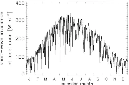
In our simulations the ROMS model was driven by an annual cycle of external ir-radiances and winds obtained from reanalysis of gridded atmospheric data at 6-hour resolution obtained from the European Centre for Medium-Range Weather Forecasts. 5

Water column heating as needed to compute mixed layer dynamics in ROMS is ob-tained from simple analytical models for band-integrated short and long-wave radiation. Figure 2 shows the daily local-noon short-wave irradiances used as inputs to ROMS. This same annual cycle was repeated for each simulation year.

2.2 The EcoSim biological model

10

EcoSim is an ecological-optical modeling system that was developed for simulations of carbon cycling and biological productivity (Bissett et al., 1999a,b, 2005, 2008). It includes four phytoplankton functional groups (FG1 is small diatoms, FG2 is large di-atoms, FG3 is large dinoflagellates, and FG4 issynechococcus), each with a charac-teristic pigment suite that varies with the group carbon-to-chlorophyll a ratio, C:Chla. 15

EcoSim spectrally-resolves the irradiance as opposed to using wavelength-integrated irradiance. This allows differential growth of different phytoplankton groups that have unique pigment suites. The properties of each functional group evolve over time as a function of light and nutrient conditions. Other EcoSim components include bac-teria, dissolved organic matter, dissolved inorganic carbon cycling and 5 nutrients 20

(NO₃,NH₄,PO₄,SiO, and FeO). The interactions between EcoSim’s components de-scribe autotrophic growth of and competition between the four phytoplankton groups, differential carbon and nitrogen cycling, nitrogen fixation, and grazing. The maximum phytoplankton growth is modulated by temperature (Eppley, 1972). Loss is effected by grazing and excretion. Grazing accounts for the majority of the biomass sink in this 25

(9)

BGD

6, 10625–10662, 2009

C. D. Mobley et al.

Title Page

Tables Figures

◭ ◮

Back Close

Full Screen / Esc

Interactive Discussion to predictions of seasonal cycles of carbon cycling and phytoplankton dynamics in the

Sargasso Sea showed that its predictions were consistent with measurement of various biological and chemical quantities at the Bermuda Atlantic Time-series Study (BATS) station (Bissett et al., 1999a).

EcoSim version 2.0 as used in the present simulations includes nutrient recycling to 5

replenish nutrients lost as particles sink below the bottom of the maximum simulation depth. Fecal material and phytoplankton sink at various rates: 0.01 mday−1 for FG1, 0.1 mday−1 for FG2, 10 mday−1 for fecal material, and no sinking for FG3, FG4 and dissolved components. When particles reach the maximum depth, their masses are converted to nutrients as follows: fecal and phytoplankton carbon are converted to 10

dissolved inorganic carbon, fecal and phytoplankton nitrogen are converted to NO₃, phosphorous is converted to PO4, silicon to SiO, and iron to FeO. The flux of nutrients

out of the bottom of the model domain is immediately converted into a corresponding influx of nutrients into the bottom of the model domain. Other modifications to EcoSim since its original publication are described in Bissett et al. (2004).

15

The absorption spectra of the phytoplankton functional groups change with light and nutrient adaptation. The four groups therefore respond differently to various wave-lengths of the available light, and each group responds differently over time. EcoSim requires spectral irradiances at 5 nm bandwidths between 400 and 700 nm in order to model the changes within each functional group and competition between them. 20

The use of spectral irradiance rather than broadband PAR in modeling phytoplankton dynamics is a distinguishing feature of EcoSim. The standard EcoSim code, which we call the analytic light (AL) version, first calls the RADTRAN (Gregg and Carder, 1990) atmospheric radiative transfer model to obtain the spectral downwelling direct and diffuse plane irradiances just beneath the sea surface for clear sky conditions. 25

(10)

BGD

6, 10625–10662, 2009

C. D. Mobley et al.

Title Page

Tables Figures

◭ ◮

Back Close

Full Screen / Esc

Interactive Discussion used to rescale the computed spectral irradiances at the sea surface. In the present

simulations, the wavelength-integrated RADTRAN irradiances are rescaled to give the current value of the ROMS short-wave irradiance as shown in Fig. 2.

The RADTRAN-computed and rescaled spectral downwelling plane irradiances just beneath the sea surface are then propagated to depth using

5

E_d(z,λ)=E_d(0,λ) exp

− Zz

0

K_d(z′,λ)d z′

(3)

and a simple model forK_d,

Kd(z,λ)=

a(z,λ)+b_b(z,λ) ¯

µ_d(z,λ) . (4)

Herea(z,λ) is the total absorption coefficient (the sum of absorption by pure water and the various particulate and dissolved components), andb_b(z,λ) is the total backscatter 10

coefficient. The phytoplankton absorption is obtained from the concentrations of the functional groups and their chlorophyll-specific absorption spectra. The backscatter coefficient is obtained from the chlorophyll-dependent model of Morel and Maritorena (2001) for Case 1 waters, using the total Chlaconcentration. The total scattering co-e_fficientb(z,λ) is obtained from the Case 1 model of Gordon and Morel (1983). The 15

mean cosine for downwelling irradiance, ¯µ_d(z,λ), is itself modeled by a simple function that merges estimates of the near-surface and asymptotic-depth mean cosines (Bissett et al., 1999b, Eqs. 18–22). The value of ¯µd at the surface is set to the cosine of the in-water solar zenith angle; the value at the maximum depth is set to 0.75, which is a typical value for oceanic asymptotic light fields. Finally, the needed scalar irradiance 20

Eo(z,λ) is obtained from the computedEd(z,λ) and the approximation

E_o(z,λ)≈Ed(z,λ)Kd(z,λ)

(11)

BGD

6, 10625–10662, 2009

C. D. Mobley et al.

Title Page

Tables Figures

◭ ◮

Back Close

Full Screen / Esc

Interactive Discussion EcoSim AL uses Eqs. (3–5) to compute the irradiance to a depth at which Ed(z,λ)

integrated from 400 to 700 nm becomes less than 1Wm−2.

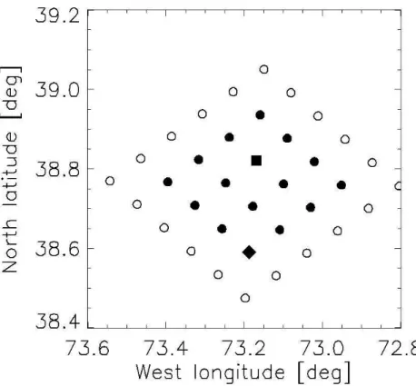
In the 6×6 grid ROMS-EcoSim code, the outer layer of grid points seen in Fig. 1 is used to impose the periodic boundary conditions. Therefore the EcoSim code com-putes the biology only at the interior 4×4 block of grid points. The biology is updated 5

at each ROMS time step and interior grid point using the analytic formulas for the scalar irradiance just described. However, the irradiances computed within EcoSim do not feed back to the ROMS code which, for programming simplicity when merging the codes, retains its original short and long-wave light parameterization for mixed-layer heating calculations. Thus the physical model influences the biology via temperature 10

and mixing, but the optical model employed within EcoSim does not influence the phys-ical model. This simplification was retained in the present study to avoid alterations to the ROMS code.

2.3 The EcoLight radiative transfer model

Accurate predictions of primary production require accurate predictions of the ambient 15

spectral scalar irradiance. Numerical models that solve the scalar RTE are currently available (Mobley et al., 1993) and can provide highly accurate predictions of the light field, in particular the scalar irradiance as a function of depth and wavelength. How-ever, the computational times required by these numerical models are far too great for their inclusion in large coupled models that need irradiance predictions at many spatial 20

locations and times of day.

The HydroLight radiative transfer model (Mobley et al., 1993; Mobley, 1994, and www.hydrolight.info) provides an accurate solution of the scalar RTE for any water body, given the inherent optical properties of the water body, the incident sky radiance, and the bottom reflectance (in finite-depth waters). Although the standard version of 25

(12)

BGD

6, 10625–10662, 2009

C. D. Mobley et al.

Title Page

Tables Figures

◭ ◮

Back Close

Full Screen / Esc

Interactive Discussion namelyN azimuthal angles for each non-polar-cap direction, plus the zenith and nadir

polar cap directions. The computational time is proportional to this number of directions squared, because each direction interacts via scattering with every other direction. A large part of the HydroLight run time is used to compute the azimuthal dependence of the radiance distribution. A slightly optimized version of HydroLight 3.1 was developed 5

by Liu et al. (1999). Liu et al. (2002) developed a multi-parameter look-up-table for scalar irradiance in homogeneous waters. Their model is based on HydroLight simu-lations and gives PAR profiles that are within a few percent of HydroLight values but runs four orders of magnitude faster. However, the Liu et al. (2002) model is not suited to the needs of EcoSim when modeling inhomogeneous or Case 2 waters.

10

Ecosystem models require only the scalar irradianceEo as a function of depth and wavelength, which is computed from an azimuthal integration of the radiance as seen in Eq. (1). The azimuthal dependence of the radiance, obtained at great computational expense in HydroLight, is thus lost in the integration of Eq. (1). This means that the RTE can be azimuthally averaged to obtain an equation for the azimuthally averaged 15

radiance as a function of polar angle. The numerical solution of the resulting RTE is much simpler than in HydroLight. In particular, there is no azimuthal decomposition of the radiance into Fourier amplitudes. OnlyM azimuthally averaged radiances need be computed, and the run time is proportional toM2. The standard version of HydroLight usesM=20 θ directions and N=24 φ directions, which gives 10 degree resolution 20

in the polar angle (including two polar caps with 5 degree half-angles) and 15 degree resolution in the azimuthal angle. Eliminating the azimuthal dependence from the cal-culations therefore gives approximately a factor-of-400 reduction in the computation time (allowing for certain calculations that are independent of angular resolution).

Based upon this observation, we developed a highly optimized version of Hydro-25

(13)

BGD

6, 10625–10662, 2009

C. D. Mobley et al.

Title Page

Tables Figures

◭ ◮

Back Close

Full Screen / Esc

Interactive Discussion nadir-viewing water-leaving radiance and remote-sensing reflectance, and diffuse

at-tenuation coe_fficients also computed by EcoLight. Although those ancillary quantities are not needed as inputs to most ecosystem models, they can be of use in ecosys-tem model validation. In particular, the water-leaving radiance and remote-sensing re-flectance allow ecosystem validation using satellite radiometric measurements without 5

the intervening step of converting radiometric measurements into chlorophyll concen-trations via imperfect chlorophyll algorithms. Quantities such as the remote-sensing reflectance are not available from the simple analytic light models.

Various additional optimizations to the EcoLight code were made. The most impor-tant are the use of a piecewise homogeneous water column, solution of the RTE to 10

di_fferent depths at di_fferent wavelengths, and wavelength skipping.

The ROMS-EcoSim code models the water column as a stack of homogeneous lay-ers of variable thickness. Therefore the IOPs within a given water layer are indepen-dent of depth. The EcoLight code takes advantage of the depth independence of the IOPs within a layer to reduce the computation needed to solve the RTE for the depth 15

dependence of the irradiances within each layer.

HydroLight solves the RTE to a user-specified geometric depth, which is the same for every wavelength and must be chosen before the run is started. This becomes compu-tationally expensive at wavelengths where the IOPs are large (e.g., at red wavelengths owing to pure water absorption or at blue wavelengths owing to CDOM absorption) cor-20

responding to a large optical depth for a given geometric depth. EcoSim requires the spectral scalar irradiance only to the bottom of the euphotic zone, below which it does not perform primary production calculations. Therefore, it is necessary to compute the irradiance only to that depth, which varies with the biological state of the ocean and cannot be predetermined.

25

(14)

BGD

6, 10625–10662, 2009

C. D. Mobley et al.

Title Page

Tables Figures

◭ ◮

Back Close

Full Screen / Esc

Interactive Discussion optical property and is not known until the RTE has been solved. However, except

very near the sea surface where boundary effects are important, Ko is roughly equal toKd, the diffuse attenuation coefficient for downwelling plane irradiance (Kobecomes exactly equal toK_d at great depths in homogeneous water). To first order (e.g., Mobley, 1994, Eq. 5.65)Kd≈a/µ¯d, wherea is the absorption coefficient and ¯µd is the mean 5

cosine of the downwelling radiance distribution. In typical waters, ¯µd≈3/4. Thus, in the modified Eq. (3) we can approximateK_o(z,λ) by the absorption coefficient a(z,λ) and define

F_o≡Eo(zo,λ)

E_o(0,λ) ≈exp

− Zz_o

0

a(z′,λ)d z′

. (6)

Given the absorption coefficient, which is known before the RTE is solved, this equation 10

can be used to estimate the depthzo at which the scalar irradiance will decrease to a fractionF_o of its surface value. Because of the approximations used, the estimatedz_o

will always be greater than the actualz_o.

At the first wavelength, zo is obtained from Eq. (6) for a pre-specified Fo, and the bottom boundary condition is then applied at this depth. At the first wavelength, λ1,

15

the RTE is solved to the estimated depth, z_o(est;λ1), determined as just described.

After the RTE is solved, the actual depth zo(exact;λ1) at which Eo(z,λ1) decreased

toFoEo(0,λ1) can be determined. At subsequent wavelengths, the ratio of actual to

estimatedz_ovalues from the previous wavelength is used to correct the initial estimate at the present wavelength:

20

zo(final;λj)=zo(est;λj)

zo(exact;λj−1)

zo(est;λj−1)

. (7)

(15)

BGD

6, 10625–10662, 2009

C. D. Mobley et al.

Title Page

Tables Figures

◭ ◮

Back Close

Full Screen / Esc

Interactive Discussion inherent in Eq. (6) becauseK_o was approximated by a. Numerical studies show that

after the first wavelength, which always goes too deep, this algorithm gives final depth estimates that are close to the actualF_o depths, as determined after solving the RTE. In practice, the RTE is solved to the next depthz_k> z_o, wherez_k,k=1,...,30 is one of the ROMS-EcoSim grid depths.

5

The computed values ofE_o(z_k) andE_d(z_k) are then accurate down to depthz_k, and they can be extrapolated to greater depths as follows. The extrapolation is based on Eq. (3), except that the mean cosine factors can now be included in the approximations forK_d≈a/µ¯_d andK_o≈a/µ¯.

In addition toE_o(z_k,λ) andE_d(z_k,λ), the solution of the RTE gives all irradiances, in 10

particular the downwelling scalar irradianceEod(zk,λ) and the upwelling plane irradi-anceE_u(z_k,λ). These irradiances are used to compute

¯

µ_d(z_k,λ)= Ed(zk,λ)

Eod(zk,λ)

and µ¯(z_k,λ)=Ed(zk,λ)−Eu(zk,λ)

Eo(zk,λ)

at the last solved depth. These values of ¯µ_d and ¯µ at depthz_k are then used at all lower depths. Thus Eq. (3) written forE_obecomes

15

E_o(z,λ)=E_o(z_k,λ) exp

− Zz

zk

a(z′,λ) ¯

µ(z_k,λ)d z

′_. ₍₈₎

A similar equation using ¯µd(zk,λ) holds for Ed. Equation (8) is then applied to the homogeneous layers beginning at depth zk and extending to the maximum depth of the ROMS-EcoSim grid.

Note thatE_o(z_k,λ) and the other irradiances incorporate all of the effects of the sur-20

face boundary and of the water IOPs above the maximum depthzk to which the RTE was solved. The extrapolations based on Eq. (8) are accurate if the variability in the ¯µ

(16)

BGD

6, 10625–10662, 2009

C. D. Mobley et al.

Title Page

Tables Figures

◭ ◮

Back Close

Full Screen / Esc

Interactive Discussion There is also an option to solve the RTE at only some wavelengths and to obtain

the irradiances at the unsolved wavelengths (needed by EcoSim) by interpolation. For example, EcoLight can solve the RTE at wavelengths 1, 3, 5... and then estimate the irradiances at wavelengths 2, 4, 6... by interpolation between the computed wave-lengths. Omitting every other wavelength gives a factor-of-two decrease in the EcoLight 5

run time, all else being equal.

In summary, EcoLight takes the following philosophy. It is necessary to solve the RTE in order to incorporate the effects of the surface boundary conditions and to account for all IOP effects. However, once an accurate value ofEo(zk,λ) has been computed to some depthz_k deep enough to be free of surface boundary effects, it is not necessary 10

to continue solving the RTE to greater depths, which is computationally expensive. As shown below, in many cases of practical interest it is possible to extrapolate the accurately computed upper-water-column irradiances to greater depths and still obtain irradiances that are acceptably accurate for ecosystem predictions. Likewise, it may not be necessary to solve the RTE at every wavelength in order to obtain acceptably 15

accurate irradiances at the needed wavelength resolution.

2.4 The ROMS-EcoSim-EcoLight coupled model

The ROMS and EcoSim models were previously coupled and that code served as the starting point for the incorporation of EcoLight. The analytic irradiance model found in the standard EcoSim code was replaced by a call to the EcoLight subroutine. EcoSim 20

passes EcoLight the current total IOPs as functions of depth and wavelength, atmo-spheric conditions (as needed by RADTRAN, which is also used by EcoLight to com-pute the spectral irradiance incident onto the sea surface), wind speed, grid depths, and other information needed by EcoLight. After solving the RTE, EcoLight returns the scalar irradianceEo(z,λ) to EcoSim for use in its primary production calculations. 25

(17)

BGD

6, 10625–10662, 2009

C. D. Mobley et al.

Title Page

Tables Figures

◭ ◮

Back Close

Full Screen / Esc

Interactive Discussion

3 Ecosystem behavior

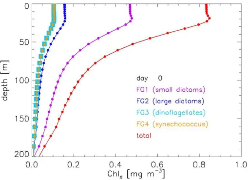
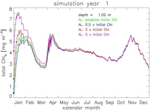
Figure 3 shows the initial chlorophyll vs. depth profiles for the four phytoplankton func-tional groups. These profiles were used as the “baseline” initial profiles for all subse-quent simulations.

We first investigated EcoSim’s biological predictions when using its original ana-5

lytic irradiance model. We expect that the long-term ecosystem behavior should be determined by the ecosystem internal structure and external forcing, and thus be in-dependent of the initial conditions. To verify this, runs were made starting with the initial chlorophyll profiles seen in Fig. 3, and with profiles that were one-half, twice, and five-times the values seen in that figure. Figure 4 shows the resulting total chlorophyll 10

concentrations (the sums of the chlorophyll concentrations for the four phytoplankton functional groups) near the sea surface for simulation year 1. For this and subsequent figures, values are plotted daily at local noon. As expected, the differences due to the initial chlorophyll profiles damp out within a few months and remain small during subsequent years. Greater depths show the same behavior, as do runs using EcoLight-15

computed irradiances.

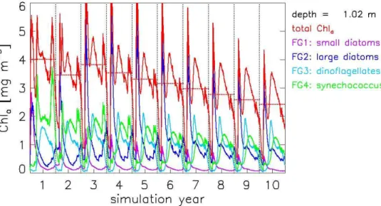
We next examined the ecosystem annual cycle for long-term simulations. A run for ten simulated years was made starting with the chlorophyll profiles of Fig. 3. The first three years show transient behavior as the ecosystem adjusts to the initial profiles and external forcing. Years 4–10 then show similar annual cycles, except for a slow year-20

to-year decrease in chlorophyl concentrations, as shown in Fig. 5. During simulation years 8 to 10, the year-to-year decrease in the annual maximum chlorophyll values is 9 to 11% for diatoms and 3 to 5% for dynoflagellates andsynechococcus, which gives an annual decrease of about 9% in the maximum total chlorophyll. The annual average chlorophyll values decrease somewhat less over the same three years, with the annual 25

(18)

BGD

6, 10625–10662, 2009

C. D. Mobley et al.

Title Page

Tables Figures

◭ ◮

Back Close

Full Screen / Esc

Interactive Discussion recycling used in EcoSim. The same behavior occurs with EcoLight irradiance

calcula-tions. Such behavior is not surprising for the limited spatial grid (which does not include horizontal advection of nutrients) and fixed particle sinking and nutrient recycling rates assumed here. The failure of the present idealized ecosystem to attain a completely stable annual cycle in no way compromises our comparisons of analytic vs numerical 5

irradiance calculations, for which all else is the same. Although we do not expect to reproduce local conditions within the limited spatial domain, it is encouraging to note that our modeled surface chlorophyll values in spring-early summer are of the same order of magnitude (1–3 mgm−3) as coincident SeaWiFs data for this area.

4 Irradiance model comparisons

10

We now consider the long-term ecosystem behavior for different ways of computing the scalar irradiance used in EcoSim for its primary production calculations. In these simulations, the time step was 9 min, which was set by ROMS for computational stabil-ity. A one-year simulation thus requires 58 400 time steps. In the baseline simulations, EcoSim updates its light and biology at each time step, although the irradiances are 15

computed only when the sun is above the horizon. Such frequent de novo recompu-tation of the in-water irradiance is not compurecompu-tationally feasible for EcoLight because of its longer run times, nor is it necessary.

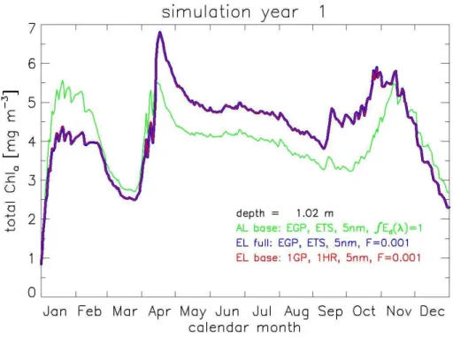
Figure 6 shows a one-year simulation with three versions for the light model called by EcoSim. The first model is the default analytic light (AL) model used by EcoSim. 20

This model computes the irradiances at every grid point (notation: EGP) and every time step (ETS) when the sun is above the horizon. Irradiances are computed at 5 nm resolution between 400 and 700 nm. Irradiances are computed down to the depth where the integratedE_d is 1 W m−2. This is the AL baseline run, which is our standard for comparison with runs that call the EcoLight model to obtain the irradiances. This AL 25

(19)

BGD

6, 10625–10662, 2009

C. D. Mobley et al.

Title Page

Tables Figures

◭ ◮

Back Close

Full Screen / Esc

Interactive Discussion biological (EcoSim) and optical (analytic or EcoLight) calculations.

The second model uses EcoLight (EL) to compute the irradiances at every grid point, every time step, and every wavelength down to a depth where the scalar irradiance decreased to 0.001 of the surface value, i.e., to a depthzocorresponding toFo=0.001 in Eq. (6), as dynamically corrected by Eq. (7). For the initial chlorophyll profiles seen in 5

Fig. 3,z_ois approximately 50 m. Below depthz_oEcoLight extrapolated the irradiances using Eq. (8). This extrapolation defines the irradiances throughout the water column (down to 210 m in these simulations), even though the values at great depths are not used by EcoSim. These EcoLight computations thus give highly accurate irradiances throughout the euphotic zone, for the IOP and sky inputs passed to EcoLight by ROMS 10

and EcoSim. This full EcoLight simulation corresponds almost exactly to the baseline conditions of the EcoSim calculations using its analytic light model. However, this run required 135 h and 35 min, which is much too long for routine calculations.

The third run shown in Fig. 6 shows the results when EcoLight was called at only one grid point (1GP) and once per simulation hour (1HR), with other options being the 15

same as in the previous EcoLight run. At time steps where EcoLight is not called, the most recently computed spectral irradiances are simply rescaled by the ratio of the cur-rent RADTRAN sky irradiance to that at the time of the previous full computation. This should give good irradiances if the IOPs have not changed greatly since the last full calculation. The irradiances at the computed grid point are rescaled in the same man-20

ner and applied at the other grid points. This should give reasonably good predictions if the IOPs are not greatly different between the grid points where the exact computation is made and where the rescaled irradiances are applied. This run required 8 h and 34 min, which although much faster than the full EL run is still too long for ecosystem modeling.

25

(20)

BGD

6, 10625–10662, 2009

C. D. Mobley et al.

Title Page

Tables Figures

◭ ◮

Back Close

Full Screen / Esc

Interactive Discussion can be called at only one grid point and once per hour without significantly altering the

ecosystem behavior compared to calling it at every ROMS grid point and every time step. Compared to the EL full model, the EL 1GP, 1HR, 5 nm,F_o=0.001 run gives the same predictions as the EL full model, but at only 6% of the run time. We therefore adopt these EL options as the baseline for subsequent EcoLight runs for ten-year sim-5

ulations. We presume that the EL runs give a better ecosystem prediction than the AL run because the EL irradiances are computed more accurately.

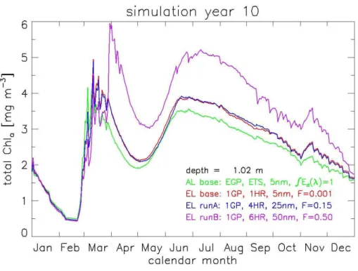
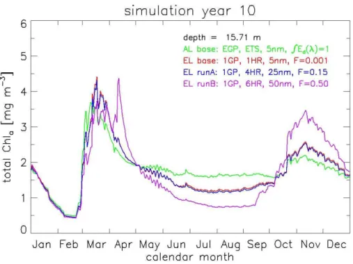
Figure 7 shows several comparisons of AL and EL runs during simulation year 10. We first note the similarity between the AL and EL base runs. (The first year of this simulation was seen in Fig. 6.) These two runs differ by no more than 23% after ten 10

years of simulation. This is a relatively small di_fference given the much di_fferent ways in which the irradiances are computed. The similarity in these two runs can be viewed in either of two ways. First, the agreement is a validation of EcoSim’s simple analytic irradiance model for Case 1 water, compared to the exact solution of the RTE for the same IOPs. Good agreement is to be expected, since the AL light model was designed 15

for use in Case 1 waters as modeled here. Alternatively, the similarity can be viewed as confirmation that the EcoLight code has been fully debugged and properly embedded within the ROMS-EcoSim code.

Since we can reduce the spatial and temporal frequency of calling EcoLight (or the analytic light model, for that matter) as just described without altering the ten-year 20

ecosystem predictions by more that one percent, the question arises as to how much more the frequency of light computations can be reduced without significantly altering the long-them ecosystem behavior. Figure 7 shows two further examples of reduced temporal, wavelength, and depth resolution in EcoLight runs for the last year of a ten-year simulation. EL Run A called EcoLight at the first ROMS time step after sunrise 25

(21)

BGD

6, 10625–10662, 2009

C. D. Mobley et al.

Title Page

Tables Figures

◭ ◮

Back Close

Full Screen / Esc

F_o=0.15, with extrapolation to deeper depths as previously described. In a similar fashion, EL Run B called EcoLight every 6 h at 50 nm resolution, and solved the RTE down to only the 50% orFo=0.5 light level.

The EL base and EL Run A simulations differ by a maximum of 4% during the tenth simulation year. Thus very little long-term difference was induced by the reduction in 5

wavelength and depth resolution for EL Run A vs. the EL base run. However, EL Run A took only 41 min per simulation year, which is just 28% more than the AL base run. EL Run B took 40 min. The small decrease in run time between EL Run A and Run B indicates that the overhead required to call and initialize EcoLight now dominates its run time, rather than the time required to solve the RTE itself. However, EL Run B 10

gives chlorophyll predictions that differ by as much as 73% after ten years, compared to the EL base run. Note also that the time of the maximum spring bloom is delayed by almost a month in EL Run B. Such differences are too large to be acceptable. Thus we view the computational frequency of EL Run A as being satisfactory, given the small increment in run time compared to the AL model, but EL Run B is not satisfactory and 15

in any case gives only a slight additional saving in run time.

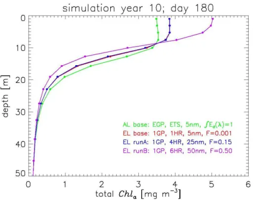
The same behavior is seen at greater depths. Figure 8 shows the year-ten time series at depth 15.7 m. At this depth, AL base and EL base differ by up to 26%. EL base and EL run A remain within 4% of each other, but EL Run B differs from Run A by up to 65%. Figure 9 shows the upper 50 m depth profile of total chlorophyll values 20

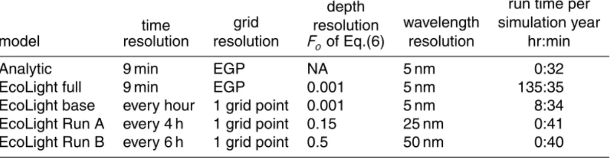
at day 180 of year 10, illustrating that the largest di_fference between the analytical and EcoLight model predictions occurs in the upper 20 m. Below this depth, both solutions converge. Table 1 summarizes these runs.

5 Conclusions

It is of course possible to try other combinations of time, wavelength, and depth res-25

(22)

BGD

6, 10625–10662, 2009

C. D. Mobley et al.

Title Page

Tables Figures

◭ ◮

Back Close

Full Screen / Esc

Interactive Discussion in ecosystem models with at most a few tens of percent increase in total run times.

Although both the analytic and EcoLight models gave comparable chlorophyll predic-tions for ten-year simulapredic-tions of open-ocean Case 1 waters, such agreement cannot be expected in simulations of Case 2 waters, for which the analytic light model is not valid. The EcoLight solution of the RTE to a given optical depth is not dependent on whether 5

the IOPs describe Case 1 or 2 water. Its fast run times seen here will therefore be retained in applications to other water bodies. A chlorophyll-based analytic light model will underestimate the scalar irradiance in simulations of optically shallow waters with bright reflective bottoms. In such waters, bottom reflectance increases the in-water scalar irradiance and proportionately affects biological productivity and water-column 10

heating rates. In optically shallow waters, it would be necessary to force EcoLight to solve the RTE all the way to the physical bottom at each wavelength in order to account for bottom reflectance effects. However, any corresponding increase in run time is a penalty worth paying if the improved irradiance computations give significantly better ecosystem predictions in such waters, and the run time will even decrease if the bottom 15

depth is less than the deep-waterz_o given by Eq. (7).

It is our view that it does not matter how fast a light model runs if its predictions are not sufficiently accurate to meet the user’s needs. EcoLight provides a numerical light model that accurately computes irradiances for any water body or boundary conditions being simulated by the associated physical-biological models. The run time increase 20

when using EcoLight in an optimized way, i.e., not calling it at every time step, every grid point, and every wavelength, is at most a few tens of percent. Moreover, EcoLight automatically provides ancillary output (not shown in this paper) such as the remote sensing reflectance, plane irradiances, and nadir- and zenith-viewing radiances, all of which can be used to verify ecosystem predictions with observational data, or which 25

(23)

BGD

6, 10625–10662, 2009

C. D. Mobley et al.

Title Page

Tables Figures

◭ ◮

Back Close

Full Screen / Esc

Interactive Discussion price to pay for potential improvements in ecosystem predictions, for extending the light

model to Case 2 and shallow waters, and for obtaining ancillary radiometric variables useful for ecosystem validation.

We thus feel that although simple analytic irradiance models do run extremely fast, there is little justification for their continued use in light of their potential inaccuracies 5

and limitations, even for Case 1 waters. Moreover, analytic models usually parameter-ize the water inherent optical properties in terms of a single quantity – the total chloro-phyll concentration – which oversimplifies the complex relation between light propaga-tion and the scattering and absorppropaga-tion properties of various ocean constituents. So-phisticated ecosystem models such as EcoSim track several phytoplankton functional 10

groups as well as other dissolved and particulate constituents, each of which has its own absorption and scattering properties. EcoSim determines total inherent optical properties as sums of the contributions by various components and is thus able to model changes in the light field induced by changes in the concentration or optical properties of whatever components are included in the biological model. Such connec-15

tions between ecosystem components and the light field cannot be well simulated by chlorophyll-based models.

Computational stability criteria of ecosystem physical models may require time steps as small as one minute, depending on grid cell size. However, it is seldom if ever nec-essary to update the light field at each time step. It appears reasonable to run EcoLight 20

at hourly or longer intervals and then interpolate to the desired time. The same idea applies to running EcoLight on a coarser spatial grid than the physical model uses and then interpolating to obtain the required spatial resolution. In practice, it should be pos-sible to dynamically determine when to call EcoLight. For example, as the calculations proceed to a new grid point, the IOPs at that grid point could be compared with those 25

(24)

BGD

6, 10625–10662, 2009

C. D. Mobley et al.

Title Page

Tables Figures

◭ ◮

Back Close

Full Screen / Esc

Interactive Discussion new grid point differ by more than some amount from those at the reference point, then

EcoLight would be called for a de novo calculation of the irradiance, and the current grid point would become the new reference point. A dynamic determination of when to call EcoLight would allow for frequent calls near fronts or in other situations where the IOPs or external properties are changing rapidly, and for few calls in fairly homogenous 5

and stable ocean regions. When employed is this manner, EcoLight should be applica-ble to large-scale three-dimensional ecosystem models requiring spectral irradiances at many wavelengths and on a fine spatial and temporal grid, but at little more compu-tational expense than calling an analytical light model at every time step and grid point, as is done in the current ROMS-EcoSim code.

10

Light is an important factor in determining primary production and mixed-layer ther-modynamics, so we expect that EcoLight’s accurately computed spectral scalar irra-diances will significantly improve ecosystem model predictions, compared to the use of approximate analytical models for spectral irradiance or PAR. Moreover, predictions of primary production in shallow waters and for sea grass beds, for which analytic 15

chlorophyll-based models can be offby large factors, would be well-served by the use of EcoLight.

The EcoLight version 1.0 code used in the present study is mostly Fortran 77 and contains HydroLight legacy features that are not needed for ecosystem simulations. We expect that a thorough rewriting of EcoLight in Fortran 95, removal of unneeded 20

features, and use of a faster RTE solver might gain another factor of two in run times for the EcoLight module. That rewrite is now under way. When ready, that code will be imbedded in a fully 3-D ecosystem model for investigation of the issues just mentioned.

Acknowledgements. Authors C. D. M. and L. K. S. were supported in this work by the US Office of Naval Research Environmental Optics Program as part of the Hyperspectral Coastal Ocean

25

Dynamics Experiment (HyCODE) and under follow-on contracts 00-D-0161, N00014-05-M-0146, and N00014-8-C-0024. Authors W. P. B. and B. C. were supported by Office of Naval Research Environmental Optics Program as part of HyCODE, under follow-on contract N00014-8-C-0024, and by the US National Science Foundation Coastal Ocean Processes La-grangian Transport and Transformation Experiment (LaTTE) under grant 0238745.

(25)

BGD

6, 10625–10662, 2009

C. D. Mobley et al.

Title Page

Tables Figures

◭ ◮

Back Close

Full Screen / Esc

Interactive Discussion References

Baker, K. S. and Frouin, R.: Relation between photosynthetically available radiation and total insolation at the ocean surface under clear skies, Limnol. Oceanogr., 32, 1370–1377, 1987. 10629

Bissett, W. P., Meyers, M. B., Walsh. J. J., and M ¨uller-Karger, F. E: The effects of temporal

5

variability of mixed layer depth on primary productivity around Bermuda, J. Geophys. Res., 99(C4), 7539–7553, 1994. 10627

Bissett, W. P., Walsh, J. J., Dieterle, D. A., and Carder, K. L.: Carbon cycling in the upper waters of the Sargasso Sea: I. Numerical simulation of differential carbon and nitrogen fluxes, Deep-Sea Res., 46, 205–269, 1999a. 10629, 10632, 10633

10

Bissett, W. P., Carder, K. L., Walsh, J. J., and Dieterle, D. A.: Carbon cycling in the upper waters of the Sargasso Sea: II. Numerical simulation of apparent and inherent optical properties, Deep-Sea Res., 46, 271–317, 1999b. 10629, 10632, 10634

Bissett, W. P, Schofield, O., Glenn, S., Cullen, J. J., Miller, W. L., Plueddemann, A. J., and Mobley, C. D.: Resolving the impacts and feedbacks of ocean optics on upper ocean ecology.

15

Oceanography, 14, 30–49, 2001.

Bissett, W. P., DeBra, S., and Dye, D.: Ecological Simulation (EcoSim) 2.0 Technical De-scription. FERI Technical Document Number FERI-2004-0002-U-D, online available at: http: //feri.s3.amazonaws.com/pubs ppts/FERI 2004 0002 U D.pdf, 10 August, 2004. 10633 Bissett, W. P., Arnone, R., DeBra, S., Dieterle, D. A., Dye, D., Kirkpatrick, G., Schofield, O.

20

M., and Vargo, G.: Predicting the optical properties of the West Florida Shelf: Resolving the potential impacts of a terrestrial boundary condition on the distribution of colored dissolved and particulate matter, Mar. Chem., 95, 199–233, 2005. 10632

Bissett, W. P., Arnone, R., DeBra, S., Dye, D., Kirkpatrick, G., Mobley, C. D., and Schofield, O. M.: The integration of ocean color remote sensing with coastal nowcast/forecast simulations

25

of harmful algal blooms (HABs), in: Real Time Coastal Observing Systems for Ecosystem Dynamics and Harmful Algal Blooms, edited by: Babin, M., Roesler, C., and Cullen, J. J., UN Educ., Sci. and Cult. Organ., Paris, 85–108, 2008. 10632

Cahill, B., Schofield, O., Chant, R., Wilkin, J., Hunter, E., Glenn, S., and Bissett, W. P.: Dynam-ics of turbid buoyant plumes and the feedbacks on nearshore biogeochemistry and physDynam-ics,

30

Geophys. Res. Lett., 35, L10605, doi:10.1029/2008GL033595, 2008. 10631

(26)

BGD

6, 10625–10662, 2009

C. D. Mobley et al.

Title Page

Tables Figures

◭ ◮

Back Close

Full Screen / Esc

Ross Sea circulation and biogeochemistry, Deep-Sea Res. II, 50, 3103–3120, 2003. 10631 Doney, S. C., Glover, D. M., and Najjar, R. G.: A new coupled, one-dimensional

biological-physical model for the upper ocean: Application to the JGOFS Bermuda Atlantic Timeseries Study (BATS) site, Deep-Sea Res. II, 43, 591–624, 1996. 10628

Eppley, R. W.: Temperature and phytoplankton growth in the sea, Fish. Bull., 70(4), 1063–1085,

5

1972. 10632

Evans, G. T. and Parslow, J. S.: A model of annual plankton cycles, Biol. Oceanogr., 3, 328– 347, 1985. 10627, 10628

Fasham, M. J. R.: Variations in the seasonal cycle of biological production in subarctic oceans: A model sensitivity analysis, Deep-Sea Res. II, 42, 1111–1149, 1995. 10628

10

Fasham, M. J. R., Ducklow, H. W., and McKelvie, S. M.: A nitrogen-based model of plankton dynamics in the oceanic mixed layer, J. Mar. Res., 48, 591–639, 1990. 10628

Fennel, K. and Wilkin, J.: Quantifying biological carbon export for the northwest North A tlantic continental shelves, Geophys. Res. Lett., in press, 2009. 10631

Fennel, K., Wilkin, J., Levin, J., Moisan, J., O’Reilly, J., and Haidvogel, D.: Nitrogen

cy-15

cling in the Middle Atlantic Bight: Results from a three-dimensional model and impli-cations for the North Atlantic nitrogen budget, Global Biogeochem. Cy., 20, GB3007, doi:10.1029/2005GB002456, 2006. 10631

Fennel, K., Wilkin, J., Previdi, M., and Najjar, R.: Denitrification effects on air-sea CO2 flux in the coastal ocean: Simulations for the Northwest North Atlantic, Geophys. Res. Lett., 35,

20

L24608, doi:10.1029/2008GL036147, 2008. 10631

Fringer, O. B, McWilliams, J. C., and Street, R. L.: A new hybrid model for coastal simulations, Oceanography, 19, 64–77, 2006.

Fujii, M., Boss, E., and Chai, F.: The value of adding optics to ecosystem models: a case study, Biogeosciences, 4, 817–835, 2007,

25

http://www.biogeosciences.net/4/817/2007/. 10630

Gordon, H. R. and Morel, A.: Remote assessment of ocean color for interpretation of satel-lite visible imagery, a review, Lecture Notes on Coastal and Estuarine Studies, 4, Springer Verlag, New York, 114 pp., 1983. 10634

Gregg, W. W. and Carder, K. L.: A simple spectral solar irradiance model for cloudless maritime

30

atmospheres, Limnol. Oceanogr., 35, 1657–1675, 1990. 10633

(27)

BGD

6, 10625–10662, 2009

C. D. Mobley et al.

Title Page

Tables Figures

◭ ◮

Back Close

Full Screen / Esc

Kyewalyanga, M., Platt, T., and Sathyendranath, S.: Ocean primary production calculated by spectral and broad-band models, Mar. Ecol.-Prog. Ser., 85, 171–185, 1992. 10628

Liu, C.-C., Woods, J. D., and Mobley, C. D.: Optical model for use in oceanic ecosystem models, Appl. Optics, 38, 4475–4485, 1999. 10636

Liu, C.-C., Carder, K. L., Miller, R. L., and Ivey, J. E.: Fast and accurate model of underwater

5

scalar irradiance, Appl. Optics, 41, 4962-4974, 2002. 10636

Lutjeharms, J. R. E., Penven, P., and Roy, C.: Modelling the shear edge eddies of the southern Agulhas Current, Cont. Shelf Res., 23, 1099–1115, 2003. 10631

Marchesiello, P., McWilliams, J. C., and Shchepetkin, A. F.: Equilibrium structure and dynamics of the California Current System, J. Phys. Oceanogr., 33(4), 753–783, 2003. 10631

10

Mobley, C. D.: Light and Water: Radiative Transfer in Natural Waters, Academic Press, San Diego, 1994. 10626, 10630, 10635, 10638

Mobley, C. D., Gentili, B., Gordon, H. R., Jin, Z., Kattawar, G. W., Morel, A., Reinersman, P., Stamnes, K., and Stavn, R. H.: Comparison of numerical models for computing underwater light fields, Appl. Optics, 32, 7484–7504, 1993. 10630, 10635

15

Moore, J. K, Doney, S. C., Kleypas, J. A., Glover, D. M., and Fung, I. Y.: An intermediate complexity marine ecosystem model for the global domain, Deep-Sea Res. II, 49, 403–462, 2002. 10628

Morel, A. and Maritorena, S.: Bio-optical properties of oceanic waters: a reappraisal, J. Geo-phys. Res., 106(C4), 7163–7180, 2001. 10634

20

Oguz, T., Ducklow, H., Malanotte-Rizzoli, P., Tugrul, S., Nezlin, N. P., and Unluata, U.: Simu-lation of annual plankton productivity cycle in the Black Sea by a one-dimensional physical-biological model, J. Geophys. Res., 101, 16585–16599, 1996. 10628

Oschlies, A. and Garc¸on, V.: An eddy-permitting coupled physical-biological model of the North Atlantic - Part I: Sensitivity to advection numerics and mixed layer physics, Global

25

Biogeochem. Cy., 13, 135–160, 1998. 10628

Paulson, C. A. and Simpson, J. J.: Irradiance measurements in the upper ocean, J. Phys. Oceanogr., 7, 952–956, 1977.

Peliz, ´A., Dubert, J., Haidvogel, D. B., and Le Cann, B.: Generation and unstable evolution of a density-driven eastern poleward current: The Iberian Poleward Current, J. Geophys. Res.,

30

108(C8), 3268, doi:10.1029/2002JC001443, 2003. 10631

(28)

BGD

6, 10625–10662, 2009

C. D. Mobley et al.

Title Page

Tables Figures

◭ ◮

Back Close

Full Screen / Esc

interpretation of results, J. Plankton Res., 19, 1637–1670, 1997. 10627

Shchepetkin, A. and McWilliams, J. C.: Quasi-monotone advection schemes based on explicit locally adaptive dissipation, Mon. Weather Rev., 126, 1541–1580, 1998. 10631

Shchepetkin, A. and McWilliams, J. C.: A method for computing horizontal pressure gradient force in an oceanic model with a nonaligned vertical coordinate, J. Geophys. Res., 108, 3090,

5

doi:10.1029/2001JC001047, 2003. 10631

Shchepetkin, A. F. and McWilliams, J. C.: The regional ocean modeling system (ROMS): a split-explicit, free-surface, topography-following-coordinate oceanic model, Ocean Model., 9, 347–404, 2005. 10631

Simpson, J. J. and Dickey, T. D.: Alternative parameterizations of downward irradiance and

10

their dynamical significance, J. Phys. Oceanogr., 11, 876–882, 1981. 10629

Steele, J. H. and Henderson, E. W.: The role of predation in plankton models, J. Plankton Res., 14(1), 157–172, 1992. 10632

Wilkin, J. L.: The summertime heat budget and circulation of southeast New England shelf waters, J. Phys. Oceanogr., 36(11), 1997–2011, 2006. 10631

15

(29)

BGD

6, 10625–10662, 2009

C. D. Mobley et al.

Title Page

Tables Figures

◭ ◮

Back Close

Full Screen / Esc

Table 1. Options used in comparison runs. Time resolution of 9 min is every ROMS time step; grid resolution of EGP is every ROMS grid point; wavelength resolution of 5 nm is every EcoSim wavelength. The run times are per year of simulation on a 2.16 GHz iMac computer.

model

time resolution

grid resolution

depth resolution

F_oof Eq.(6)

wavelength resolution

run time per simulation year

hr:min

(30)

BGD

6, 10625–10662, 2009

C. D. Mobley et al.

Title Page

Tables Figures

◭ ◮

Back Close

Full Screen / Esc

(31)

BGD

6, 10625–10662, 2009

C. D. Mobley et al.

Title Page

Tables Figures

◭ ◮

Back Close

Full Screen / Esc

(32)

BGD

6, 10625–10662, 2009

C. D. Mobley et al.

Title Page

Tables Figures

◭ ◮

Back Close

Full Screen / Esc

(33)

BGD

6, 10625–10662, 2009

C. D. Mobley et al.

Title Page

Tables Figures

◭ ◮

Back Close

Full Screen / Esc

(34)

BGD

6, 10625–10662, 2009

C. D. Mobley et al.

Title Page

Tables Figures

◭ ◮

Back Close

Full Screen / Esc

(35)

BGD

6, 10625–10662, 2009

C. D. Mobley et al.

Title Page

Tables Figures

◭ ◮

Back Close

Full Screen / Esc

(36)

BGD

6, 10625–10662, 2009

C. D. Mobley et al.

Title Page

Tables Figures

◭ ◮

Back Close

Full Screen / Esc

(37)

BGD

6, 10625–10662, 2009

C. D. Mobley et al.

Title Page

Tables Figures

◭ ◮

Back Close

Full Screen / Esc

(38)

BGD

6, 10625–10662, 2009

C. D. Mobley et al.

Title Page

Tables Figures

◭ ◮

Back Close

Full Screen / Esc