Coupling statistically downscaled GCM outputs with a basin-lake hydrological model in subtropical South America: evaluation of the influence of large-scale precipitation changes on regional hydroclimate variability

(1)

HESSD

7, 9523–9565, 2010

Coupling statistically downscaled GCM

outputs with a basin-lake model

M. Troin et al.

Title Page

Abstract Introduction

Conclusions References

Tables Figures

◭ ◮

Back Close

Full Screen / Esc

Printer-friendly Version

Interactive Discussion

Discussion

P

a

per

|

Dis

cussion

P

a

per

|

Discussion

P

a

per

|

Discussio

n

P

a

per

|

Hydrol. Earth Syst. Sci. Discuss., 7, 9523–9565, 2010 www.hydrol-earth-syst-sci-discuss.net/7/9523/2010/ doi:10.5194/hessd-7-9523-2010

Hydrology and Earth System Sciences Discussions

This discussion paper is/has been under review for the journal Hydrology and Earth System Sciences (HESS). Please refer to the corresponding final paper in HESS if available.

Coupling statistically downscaled GCM

outputs with a basin-lake hydrological

model in subtropical South America:

evaluation of the influence of large-scale

precipitation changes on regional

hydroclimate variability

M. Troin1, M. Vrac2, M. Khodri3, C. Vallet-Coulomb1, E. Piovano4, and

F. Sylvestre1

1

CEREGE, Aix-Marseille Universit é, CNRS, IRD, Europ ôle m éditerran éen de l’Arbois BP 80 13545 Aix-en-Provence cedex 4, France

2

(2)

HESSD

7, 9523–9565, 2010

M. Troin et al.

Title Page

Tables Figures

◭ ◮

Back Close

Full Screen / Esc

Discussion

P

a

per

|

Dis

cussion

P

a

per

|

Discussion

P

a

per

|

Discussio

n

P

a

per

|

3

LOCEAN, Paris 7 Universit ´e, IRD, CNRS, MNHN, UPMC/IPSL, Tour 45–55, 4. ´etage, 4 place Jussieu, 75252 Paris cedex 5, France

4

CICTERRA-CIGeS, Universidad Nacional de C ´ordoba, Av. Velez Sarsfield 1611, X5016GCA – C ´ordoba, Argentina

Received: 2 December 2010 – Accepted: 7 December 2010 – Published: 10 December 2010 Correspondence to: M. Troin ([email protected])

(3)

HESSD

7, 9523–9565, 2010

M. Troin et al.

Title Page

Tables Figures

◭ ◮

Back Close

Full Screen / Esc

Discussion

P

a

per

|

Dis

cussion

P

a

per

|

Discussion

P

a

per

|

Discussio

n

P

a

per

|

Abstract

We explore the reliability of large-scale climate variables, namely precipitation and tem-perature, as inputs for a basin-lake hydrological model in central Argentina. We used data from two regions in NCEP/NCAR reanalyses and three regions from LMDZ model simulations forced with observed sea surface temperature (HadISST) for the last 50

5

years. Reanalyses data cover part of the geographical area of the Sali-Dulce Basin (region A) and a zone at lower latitudes (region B). The LMDZ selected regions repre-sent the geographical area of the Sali-Dulce Basin (box A), and two areas outside of the basin at lower latitudes (boxes B and C). A statistical downscaling method is used to connect the large-scale climate variables inferred from LMDZ and the reanalyses,

10

with the hydrological Soil Water Assessment Tool (SWAT) model in order to simulate the Rio Sali-Dulce discharge during 1950–2005. The SWAT simulations are then used to force the water balance of Laguna Mar Chiquita, which experienced an abrupt level rise in the 1970’s attributed to the increase in Rio Sali-Dulce discharge. Despite that the lowstand in the 1970’s is not well reproduced in either simulation, the key

hydro-15

logical cycles in the lake level are accurately captured. Even though satisfying results are obtained with the SWAT simulations using downscaled reanalyses, the lake level are more realistically simulated with the SWAT simulations using downscaled LMDZ data in boxes B and C, showing a strong climate influence from the tropics on lake level fluctuations. Our results highlight the ability of downscaled climatic data to

repro-20

duce regional climate features. Laguna Mar Chiquita can therefore be considered as an integrator of large-scale climate changes since the forcing scenarios giving best re-sults are those relying on global climate simulations forced with observed sea surface temperature. This climate-basin-lake model is a promising approach for understanding and simulating long-term lake level variations.

(4)

HESSD

7, 9523–9565, 2010

M. Troin et al.

Title Page

Tables Figures

◭ ◮

Back Close

Full Screen / Esc

Discussion

P

a

per

|

Dis

cussion

P

a

per

|

Discussion

P

a

per

|

Discussio

n

P

a

per

|

1 Introduction

Improving the understanding of climate change has become a major challenge in southeastern South America (SESA) region, where environmental impacts are ex-pected to produce important and immediate costs on local economy and society. While the first three quarters of the 20th century were affected by prolonged drought time

pe-5

riod, this region has experienced an unprecedented humid phase since the early 1970’s (Garcia and Vargas, 1998; Garcia and Mechoso, 2005; Pasquini et al., 2006). This still ongoing wet period results from an increase in precipitation and a higher frequency and severity of extreme hydrologic events in both the Paran ´a-Plata Basin and central Argentina (Genta et al., 1998; Camilloni and Barros, 2003; Berbery and Barros, 2003;

10

Planchon and Rosier, 2005).

Laguna Mar Chiquita (30◦54′S–62◦51′W), the terminal saline lake of a 127 000 km2 catchment area in central Argentina, west of the Paran ´a-Plata Basin, has clearly expe-rienced the 20th century hydroclimatic changes through an abrupt water level rise in the early 1970’s. Such abrupt and persistent lake level rise is without precedent over

15

the last millennium according to paleolimnological reconstruction based on lacustrine archives (Piovano et al., 2002; Sylvestre et al., 2010). A recent study was conducted to assess and simulate the lake level response to regional climate and runoffvariability (Troin et al., 2010). The results pointed out to the dominant contribution of the northern Rio Sali-Dulce Basin in the early 1970’s lake level rise, suggesting a tropical climatic

in-20

fluence. An integrated basin-lake hydrological approach combining the watershed Soil Water Assessment Tool (SWAT) model with the lake water balance was then developed (Troin et al., 2010). This latter has demonstrated the performance of this coupled hy-drological model to simulate the lake level fluctuations during the 1970’s hydroclimatic transition. In this paper, we want to go a step further. The major objective is to provide

25

(5)

HESSD

7, 9523–9565, 2010

M. Troin et al.

Title Page

Tables Figures

◭ ◮

Back Close

Full Screen / Esc

Discussion

P

a

per

|

Dis

cussion

P

a

per

|

Discussion

P

a

per

|

Discussio

n

P

a

per

|

projecting and understanding future global climatic changes and their impacts on hy-drological systems. Although results vary between studies, hyhy-drological models driven directly by raw outputs of GCMs performed poorly and the predicted runoffis often over-simplified (Wilby et al., 1999; Xu, 1999). The spatial resolution of the present GCMs is too coarse to resolve local-scale processes, precluding their direct use in hydrological

5

models (Wilks and Wilby, 1999; Prudhomme et al., 2002). In particular, the reproduc-tion of observed spatial patterns of precipitareproduc-tion (Salath ´e, 2003) and daily precipitareproduc-tion variability (B ¨urger and Chen, 2005) is not su_fficient. Thus, considerable e_fforts have been made in the climate community in order to develop downscaling methods, to over-come the gap between large- and local-scale climate data required for hydrological

10

models (Wilby et al., 1999; Hay et al., 2002; Hay and Clark, 2003; Chiew et al., 2010). The most widely used are classified into dynamical and statistical approaches. The first approach refers to the regional climate models (RCMs). Resolving the physical equations of the atmospheric regional dynamics, RCMs are meteorologically and hy-drologically consistent but also computationally expensive in the production of regional

15

simulations (Tisseuil et al., 2010). Wood et al. (2004) have found that RCMs do not lead to large improvement in hydrological simulations relative to using GCMs outputs alone. In the statistical approach, statistical downscaling methods (SDMs) are used to generate local-scale climate variables from large-scale climate variables derived from GCMs outputs or reanalyses. In the usual SDMs, such as regression models (e.g.,

20

Wilby et al., 2002; Vrac et al., 2007a, Huth et al., 2008), weather typing schemes (e.g., Mamassis and Koutsoyiannis, 1996; Vrac et al., 2007b), and stochastic weather gener-ators (e.g., Wilks and Wilby, 1999; Vrac and Naveau, 2007), the fundamental concept is to relate one or several large-scale climate variables (the predictors) from GCMs or reanalyses to local-scale climate variables (the predictands). While most of the SDMs

25

(6)

HESSD

7, 9523–9565, 2010

M. Troin et al.

Title Page

Tables Figures

◭ ◮

Back Close

Full Screen / Esc

Discussion

P

a

per

|

Dis

cussion

P

a

per

|

Discussion

P

a

per

|

Discussio

n

P

a

per

|

some interest in the use of PDMs such as computational efficiency and stronger rela-tions to the local-scale climate, which seem to o_ffer a more robust way for assessing climate impacts on hydrological systems (Fowler et al., 2007).

In this context, our study aims at assessing the applicability of the integrated basin-lake hydrological model forced by statistically downscaled large-scale climate

vari-5

ables. To do so, we use a PDM approach for simulating the lake level variations of Laguna Mar Chiquita during the 1970’s hydroclimatic transition. The large-scale times series are data fields derived from the National Center for Environmental Pre-diction (NCEP)/National Center for Atmospheric Research (NCAR) reanalyses and the LMDZ GCM. The LMDZ GCM corresponds to the atmospheric component of the

IPSL-10

CM4 coupled model of the Institut Pierre Simon Laplace developed at Laboratoire de M ´et ´eorologie Dynamique (Marti et al., 2005; Dufresne et al., 2005).

Doing so, we will address the following questions: (1) Is it relevant to force a rainfall-runo_ffmodel by downscaled NCEP/NCAR reanalyses and LMDZ GCM outputs? Are the GCMs projections reliable at a local-scale?; (2) Did the large-scale simulated

pre-15

cipitations forced by observed sea surface temperature (HadSST1) for that period rep-resent the climatic control of the lake level fluctuations? If so, can Laguna Mar Chiquita be considered as an integrator of global climate variability in the SESA?

After a brief description of the area of study (Sect. 2), the five large-scale times se-ries derived from the reanalyses regions and LMDZ boxes are presented (Sect. 3). In

20

Sect. 4, the methodology used to generate rainfall-runoffsimulations is described as well as lake-level simulations. In Sect. 5, the downscaling method performance is anal-ysed during the calibration and validation periods, and the simulations are evaluated. Then, in Sect. 6, we discuss the ability of our approach to reproduce regional climate features and the Laguna Mar Chiquita fluctuations over the 1950–2005 time period.

(7)

HESSD

7, 9523–9565, 2010

M. Troin et al.

Title Page

Tables Figures

◭ ◮

Back Close

Full Screen / Esc

Discussion

P

a

per

|

Dis

cussion

P

a

per

|

Discussion

P

a

per

|

Discussio

n

P

a

per

|

2 General description of the study area

2.1 The lake watershed

Laguna Mar Chiquita (30◦54′S–62◦51′W) is a hydrologically closed terminal lake oc-cupying a tectonic depression that formed during the middle Pleistocene (Krohling and Iriondo, 1999). The lake catchment is estimated to 127 000 km2 from 26◦S to 32◦S

5

and from 62◦W to 66◦W (Fig. 1), with a relatively low relief except for its mountainous borders on the northwest and southwest, called Sierras de Aconquija and Pampeanas ranges, respectively. The lake catchment is part of the Chaco-Pampean Plain, a larger lowland area where grasslands and shrublands have been modified for agricultural ac-tivities during the last century (Gavier and Bucher, 2004).

10

2.2 Hydrology of Laguna Mar Chiquita

Laguna Mar Chiquita is fed by three rivers (Fig. 1) and likely receives substantial groundwater inputs. The main surface water inflow is from the Rio Sali-Dulce Basin which controls 92% of lake level variations (Troin et al., 2010). The Rio Sali-Dulce Basin, covering roughly 23 810 km2 from 26◦S to 28◦S and 64◦W to 66◦W, drains the

15

northern part of the lake basin. It is the collector of many rivers that come from the Sierra de Aconquija until joining the Rio Hondo reservoir, created in 1967 to control and regulate the water distribution and also to produce hydroelectric power (Fig. 1). The hydrographic network of the Sali-Dulce Basin provides ressources necessary to the regional socio-economic development. Other minor inflows to the lake, draining

20

(8)

HESSD

7, 9523–9565, 2010

M. Troin et al.

Title Page

Tables Figures

◭ ◮

Back Close

Full Screen / Esc

Discussion

P

a

per

|

Dis

cussion

P

a

per

|

Discussion

P

a

per

|

Discussio

n

P

a

per

|

2.3 Regional climate

Characterized by a wet season (with high precipitation and temperature) from Decem-ber to March and a dry season between June and August, the studied area is sub-jected to a latitude climate gradient. In the south, around Laguna Mar Chiquita, the climate is warm-temperate (mean annual temperature of 18◦C) with mean annual

pre-5

cipitation of 806 mm. Northward, the Sali-Dulce Basin is rather characterized by a subtropical climate (mean annual temperature of 20◦C) with mean annual precipitation of 1300 mm. In the northern part of the Sali-Dulce Basin, orographic precipitations exceeding 1500 mm per year are observed.

The major atmospheric features driving seasonal climatic variability in the SESA

10

is the South American Monsoon System (SAMS). In the austral summer, the SAMS extends southward from the tropical continental region connecting the tropical Atlantic Inter Tropical Convergence Zone (ITCZ) with the South Atlantic Convergence Zone (SACZ) through a large-scale atmospheric circulation containing a low-level jet (Zhou and Lau, 1998). The South American low-level jet originating in the northern part of

15

South America at the foot of the Andes is driven by the Chaco Low to provide moisture for the SESA, bringing vapor from the tropics to the subtropical latitudes (Labraga et al., 2000; Barros et al., 2002). In contrast, the SACZ displays a weak convective activity during the austral winter and rainfall regime deceases excepted at the East in SESA where the South East trade wind circulation brings moisture associated with

20

local rainfall (Barros et al., 2002).

3 Data

3.1 Local-scale meteorological and hydrological data

Meteorological data in the lake basin for the 1950–2005 time period were obtained from the Direcci ´on Provincial de Agua y Saneamiento (DIPAS) in Argentina’s C ´ordoba

(9)

HESSD

7, 9523–9565, 2010

M. Troin et al.

Title Page

Tables Figures

◭ ◮

Back Close

Full Screen / Esc

Discussion

P

a

per

|

Dis

cussion

P

a

per

|

Discussion

P

a

per

|

Discussio

n

P

a

per

|

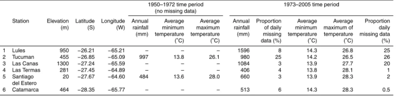
Province, the Instituto Nacional de Tecnologia Agropecuaria (INTA), the National Cli-matic Data Center (NCDC), and CLARIS LPB project database (http://www.claris-eu. org/). It consists of daily minimum and maximum temperatures and precipitation for two stations during the 1950–2005 time period and four stations for 1973–2005 in the Sali-Dulce Basin (Fig. 1 and Table 1).

5

Monthly river discharge was obtained from Argentina’s Subsecretar´ıa de Recursos H´ıdricos and the Laboratorio de Hidr ´aulica at the Universidad Nacional de C ´ordoba (Ta-ble 2). The Rio Sali-Dulce is gauged after the reservoir at the Hondo station (Fig. 1), and a time series was obtained by combining two neighbouring gauging stations, which were well correlated during the 1967–1982 common time period (r2₌0.99). The

10

Hondo gauging station covers the drainage area to the reservoir, e.g. 98% of the total Sali-Dulce Basin area (Fig. 1 and Table 2).

3.2 Large-scale meteorological data

3.2.1 Reanalysis data

NCEP/NCAR reanalysis data are atmospheric model outputs derived from the

assim-15

ilation of surface observation stations, upper-air stations and satellite-observing plat-forms with long records starting in 1948 and continuing to present day. These data are typically viewed as observed large-scale data on a regular grid with a spatial resolu-tion of 2.5 by 2.5 degrees in longitude and latitude direcresolu-tions. In this work, mean daily minimum and maximum temperatures and precipitation from two regions during the

20

(10)

HESSD

7, 9523–9565, 2010

M. Troin et al.

Title Page

Tables Figures

◭ ◮

Back Close

Full Screen / Esc

Discussion

P

a

per

|

Dis

cussion

P

a

per

|

Discussion

P

a

per

|

Discussio

n

P

a

per

|

3.2.2 General circulation model simulations

The GCM used is the LMDZ version 4, the atmospheric component of the IPSL-CM4 coupled model of the Institut Pierre Simon Laplace (Marti et al., 2005), developed at Laboratoire de M ´et ´eorologie Dynamique, and used to produce climate change simu-lations for the 2007 IPCC report (Dufresne et al., 2005). The model is formulated in

5

the finite-difference grid with a horizontal resolution of 3.75 by 2.5 degrees in longi-tude and latilongi-tude directions and 19 hydrid vertical layers (Hourdin et al., 2006). Using this model, we performed an ensemble of ten simulations forced by the observed sea surface temperature from 1951 to 2005, using the monthly HadSST1 global dataset (Rayner et al., 2003). Each simulation member only di_ffers from the sea ice and sea

10

surface temperature used as initial conditions.

Daily minimum and maximum temperatures and precipitation averaged over the 10 members ensemble were then extracted for three regions from the model outputs, re-ferred as box A (from 25◦S to 35◦S and 55◦W to 67◦W), box B (from 15◦S to 25◦S and 55◦W to 65◦W), and box C (from 20◦S to 25◦S and 55◦W to 65◦W). Box A covers

15

the geographical area of lake basin, while the two others are located slightly north to the Sali-Dulce Basin, in order to put more emphasis on the possible tropical influence over the basin-lake hydrological evolution.

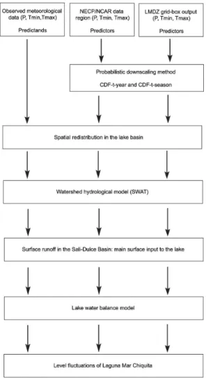
4 Methodology

The compiled data sets were used to develop five climate scenarios to investigate the

20

potential reliability of downscaled data for generating discharge scenarios in the Rio Sali-Dulce Basin for the 1950–2005 time period. The description of the methodologies involved will follow the routes shown in the Fig. 2. Daily precipitation and temperature time series produced from probabilistically downscaled NCEP/NCAR reanalyses and LMDZ outputs were distributed spatially over the Sali-Dulce Basin in order to fit with the

25

(11)

HESSD

7, 9523–9565, 2010

M. Troin et al.

Title Page

Tables Figures

◭ ◮

Back Close

Full Screen / Esc

Discussion

P

a

per

|

Dis

cussion

P

a

per

|

Discussion

P

a

per

|

Discussio

n

P

a

per

|

data were then used as input to the watershed hydrological SWAT model (Arnold et al., 1998; Neitsch et al., 2002) in order to simulate the main surface runoff that feed the lake for the 1950–2005 time period. At last, the level fluctuations of Laguna Mar Chiquita were simulated during the studied period by a lake water balance model (Troin et al., 2010) forced by the outputs of SWAT. The following sections provide details of

5

the methodology involved at each stage of the analysis.

4.1 Probabilistic downscaling method

Probabilistic downscaling methods (PDMs) involve modelling relationships between statistical characteristics of the predictors and those of the predictands. Predictor vari-ables provide information concerning the daily large-scale state of the atmosphere,

10

while predictands represent the local-scale variables to be modelled such as temper-ature and precipitation that are observed at meteorological stations. In this work, the predictor variables included daily precipitation and maximum and minimum tempera-tures. The statistical relationships between predictors and predictands were modeled using the “cumulative distribution function-transform” (CDF-t) method (Michelangeli et

15

al., 2009). The cumulative distribution functionF (CDF) of a random variable X cor-responds to the probability that a random realization ofX is equal to or lower than a given valuex: F(x)=Proba(X≤x). The CDF-t method can be seen as an extension

of the quantiles-matching method (D ´equ ´e, 2007) that uses non-parametric correspon-dences between predictors and predictands quantiles. The CDF-t approach is based

20

on the assumption that a mathematical transformation t allows to translate the CDF of the predictor (e.g. temperature and precipitation from reanalyses or LMDZ) into the CDF representing the predictand (e.g. temperature and precipitation at a meteorologi-cal station). CDF-t has the advantage to take into account the change in the large-smeteorologi-cale CDF from the observed period to the future one, that is required in a changing climate

25

context (Michelangeli et al., 2009).

(12)

HESSD

7, 9523–9565, 2010

M. Troin et al.

Title Page

Tables Figures

◭ ◮

Back Close

Full Screen / Esc

Discussion

P

a

per

|

Dis

cussion

P

a

per

|

Discussion

P

a

per

|

Discussio

n

P

a

per

|

binomial distribution of the large-scale daily rainfall occurrences is often biased (in re-analyses or GCM outputs) in comparison to local observations. Hence, a threshold was defined to work on corrected large-scale occurrences distributions similar to the observed ones. In the following, we will consider that a daily local observation of rain corresponds to a wet day only if the observed intensity is 1mm or higher. Otherwise, it

5

is considered as a dry day. Then, for each given stationS, a large-scale thresholdt_Sis determined such that we have as many large-scale dry days – i.e., with large-scale rain intensities lower thant_S – as the number of observed dry days at stationS. In other words, ifF_Sis the CDF of the rain intensity (including values lower than 1 mm day−1) at stationS, andF_Lthe equivalent for the large scale data, thent_Sis determined such that

10

F_L(t_S)₌F_S(1). Hence, based on this threshold, a large-scale sequence of rain occur-rences can be obtained. Then, the large-scale values of the days where occuroccur-rences were determined (i.e., with rainfall≥t_Smm) are downscaled using CDF-t.

Because the temperatures are continuous without real bounds in this study, the daily distributions of the large-scale minimum and maximum temperatures derived from

re-15

analyses and LMDZ were directly downscaled using CDF-t.

The precipitation and temperature downscaling procedures were applied in consid-ering either all season grouped together or a seasons differentiation. Those two ap-proaches are referred in the following as CDF-t-year and CDF-t-season, respectively. In the latter, the seasons were determined based on the observed seasonality, i.e., wet

20

(November to April) and dry (May to October) seasons.

4.2 SWAT model description

The hydrological Soil and Water Assessment Tool (SWAT) model (Arnold et al., 1998; Neitsch et al., 2002) was used in this study. SWAT is a continuous-time, spatially semi-distributed hydrological watershed-scale model that operates on a daily time step. The

25

(13)

HESSD

7, 9523–9565, 2010

M. Troin et al.

Title Page

Tables Figures

◭ ◮

Back Close

Full Screen / Esc

Discussion

P

a

per

|

Dis

cussion

P

a

per

|

Discussion

P

a

per

|

Discussio

n

P

a

per

|

river network. Each sub-basin is divided in multiple Hydrologic Response Units (HRUs) that represent a unique combination of land cover, soil, and slope. The minimum cli-matic variables required for SWAT are precipitation, maximum and minimum temper-atures. For a given time step, the contribution to discharge at each sub-basin outlet is controlled by the HRU water balance calculation. The second phase is the routing

5

phase which determines the movement of water through the river network towards the basin outlet (Neitsch et al., 2002). The HRU water balance is expressed as follows:

W_t₌W_o₊ t

X

i=1

(P_i−Q_isurf−ET_i−w_iseep−Q_igw) (1)

whereW_t is the soil moisture content at the time t (in mm of water); W_o is the initial soil moisture content (mm of water);P_i is the amount of precipitation on dayi (mm of

10

water);Q_isurfis the amount of surface runoffon dayi (mm of water); ET_i is the amount of evapotranspiration on dayi (mm of water);w_iseepis the amount of percolated water through the soil profile (mm of water); andQ_igw is the amount of groundwater flow on dayi (mm of water).

Surface runoffwas estimated using the Soil Conservation Service (SCS) curve

num-15

ber procedure (SCS, 1972) and the potential evapotranspiration (PET) was determined by the Hargreaves method (Hargreaves and Samini, 1985). More details can be found in the SWAT User’s Manual (Neitsch et al., 2002).

A detailed analysis of SWAT application to the Sali-Dulce Basin is provided in Troin et al. (2010). The SWAT peformance for simulating the surface runoffis evaluated at

20

(14)

HESSD

7, 9523–9565, 2010

M. Troin et al.

Title Page

Tables Figures

◭ ◮

Back Close

Full Screen / Esc

Discussion

P

a

per

|

Dis

cussion

P

a

per

|

Discussion

P

a

per

|

Discussio

n

P

a

per

|

through:

NSE=

n

P

i=l

Q_o−Q_o

2

−

n

P

i=l

(Q_s−Q_o)2

n

P

i=l

Q_o−Q_o2

(2)

whereQ_sis the observed runoff(m3s−1);Q_sis the simulated runoff(m3s−1); andQ_sis the mean observed runoff(m3s−1).

4.3 Lake water balance model

5

A modeling study of lake level fluctuations in Laguna Mar Chiquita was recently per-formed (Troin et al., 2010). This study presented a water balance model able to sim-ulate the lake level variations in response to local climate and observed monthly river discharge in its upper catchment (see location of gauging stations in Fig. 1). A de-tailed analysis of the lake model calibration and implementation is provided in Troin et

10

al. (2010). The dynamic lake water balance of Laguna Mar Chiquita is simulated as follows:

δV

δT =A(V)(P−E)+Qin−γ with Qin=QR1+QR2+QR3 (3)

where, for the monthly time step _∆t, _∆V is the lake volume variation (m3); A is the lake area (m2), as a function of the lake volumeV;P is the on-lake precipitation (m)

15

estimated from the six rainfall stations surrounding the lake (Fig. 1);E is the evapora-tion from the lake’s surface (m) calculated using the Complementary Relaevapora-tionship Lake Evaporation (CRLE) Model (Morton, 1983; DosReis and Dias, 1998);Q_in is the water inflow from the catchment (m3); Q_R1 andQ_R2 the two southern river discharges; and

Q_R3 the Rio Sali-Dulce discharge, representing 90% of Q_in (Fig. 1). The

correspond-20

(15)

HESSD

7, 9523–9565, 2010

M. Troin et al.

Title Page

Tables Figures

◭ ◮

Back Close

Full Screen / Esc

Discussion

P

a

per

|

Dis

cussion

P

a

per

|

Discussion

P

a

per

|

Discussio

n

P

a

per

|

5 Results

5.1 Evaluation of the downscaling method

When calibrated during the 1973–1989 time period using the six observed data sets for both NCEP/NCAR reanalyses regions, CDF-t-year and CDF-t-season generally ex-plained between 37 and 75% and between 48 and 74%, respectively, of the percentage

5

of explained variance (E%) in daily maximum and minimum temperatures (Table 3). Slightly lower values were obtained from the three LMDZ boxes with a E% statis-tic between 37 and 61% and between 40 and 59%, respectively, for CDF-t-year and CDF-t-season (Table 4). Minimum temperatures were downscaled with more efficiency than maximum temperatures for both CDF-t-year and CDF-t-season and whatever the

10

downscaled large-scale data (i.e. NCEP/NCAR reanalyses regions or LMDZ boxes) (Tables 3 and 4). Minimum and maximum temperatures were better reproduced during austral spring (SON) and automn (MAM) than austral winter (JJA) and summer (DJF). From the Tables 3 and 4, it was evident that, on average, the PDM overestimated the yearly and seasonal occurrences of dry day while wet day occurences were

un-15

derestimated, whatever the downscaled large-scale data (i.e. NCEP/NCAR reanalyses regions and LMDZ boxes) and the downscaling method (i.e. year and CDF-t-season). The proportions of dry and wet days occurrences were better reproduced during austral summer (DJF) except for region B (CDF-t-year and CDF-t-season), and boxes B (CDF-t-year) and C (CDF-t-season), where the precipitation occurrences were

20

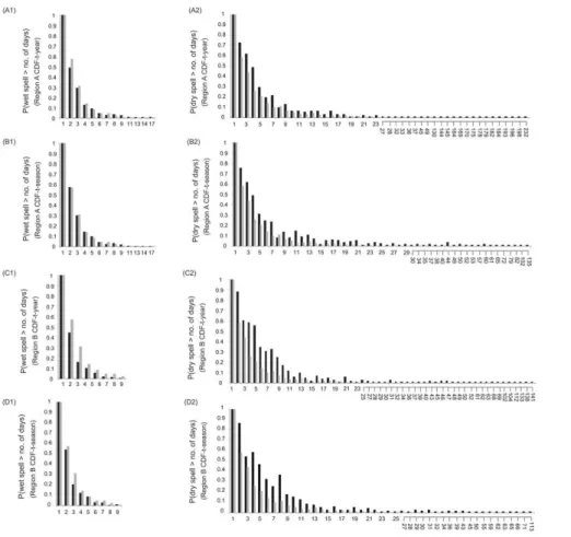
better represented, during austral spring (SON) and winter (JJA), respectively for the two boxes. Additionaly, simulated precipitation consistently reproduced the probability of observed wet and dry spells, even for small values of probabilities, corresponding to long periods (Figs. 3 and 4). Again, a tendency to underestimate the wet spell probabilities and overestimate the dry spell probabilities was observed.

25

(16)

HESSD

7, 9523–9565, 2010

M. Troin et al.

Title Page

Tables Figures

◭ ◮

Back Close

Full Screen / Esc

Discussion

P

a

per

|

Dis

cussion

P

a

per

|

Discussion

P

a

per

|

Discussio

n

P

a

per

|

stations (Table 1). Even though the percentage of wet days remained underestimated for the NCEP/NCAR reanalysis regions and the LMDZ boxes during both the PDM validation periods, the annual precipitation totals were quite similar to the observed one, especially for the boxes B and C (Tables 5 and 6). The downscaled maximum and minimum temperatures were under- and over-estimated, respectively, from both the

5

reanalysis regions and LMDZ boxes (Tables 5 and 6). It is noteworthy that a season differentiation did not allow a clear improvement of the downscaled local climate.

5.2 Comparison of rainfall-runoffsimulations

In this section, we compared the SWAT performance to simulate the Rio Sali-Dulce discharge forced by the downscaled daily precipitation and temperature derived from

10

reanalysis regions and LMDZ boxes over the PDM calibration (1973–1989) and valida-tion periods (1950–1972; 1990–2005). Addivalida-tional figures presenting the scatter plots of measured versus simulated monthly runoffover the PDM calibration and validation periods can be found in Appendixes A to F.

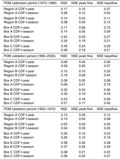
Accordingly, Table 7 showed the corresponding Nash-Sutcliffe coefficient of effi

-15

ciency (NSE) statistics for both downscaled reanalyses regions and LMDZ boxes used as input data to SWAT over the PDM calibration and validation periods.

For SWAT simulations obtained using the downscaled reanalysis regions during the PDM 1973–1989 calibration time period, the best results were found for region A with the CDF-t-season method (Table 7). However, more satisfying results were observed

20

using the downscaled LMDZ boxes B and C with a better SWAT skill using the CDF-t-year (Table 7). Additionally, the resulting NSE shows more satisfactory results for baseflow than for peak flow due to the better PDM skill in reproducing the dry climate, whatever the rainfall-runoffsimulation and the downscaling method (i.e. CDF-t-year or CDF-t-season).

25

(17)

HESSD

7, 9523–9565, 2010

M. Troin et al.

Title Page

Tables Figures

◭ ◮

Back Close

Full Screen / Esc

Discussion

P

a

per

|

Dis

cussion

P

a

per

|

Discussion

P

a

per

|

Discussio

n

P

a

per

|

periods, respectively (Table 7). However, SWAT simulations using the boxes B and C with CDF-t-year still provided the most satisfying results (Table 7).

For each SWAT simulation over the 1950–2005 time period, the model generally reproduced seasonal and annual variations in runoffof the Sali-Dulce Basin (Fig. 5). Whereas the monthly baseflow simulations driven by the downscaled reanalysis

re-5

gions and LMDZ boxes were generally accurately reproduced, peak flows remained clearly overestimated. In particular, similar findings for consecutive years (1981–1982 and 1998–1999) were noticeable for SWAT simulations using the downscaled large-scale data, especially for the region B, and the boxes A and C (Fig. 5).

5.3 Comparison of lake level simulations

10

Since, the Rio Sali-Dulce discharge was shown to be the main driver of the abrupt level rise observed in the 1970’s in Laguna Mar Chiquita (Troin et al., 2010), we used the ten simulations of Rio Sali-Dulce discharges to replace the measuredQ_R3 time series (Eq. 3). All the others components of the lake water balance model were derived from observations except for the lake evaporation which was estimated by the CRLE model

15

(Troin et al., 2010).

Generally, the trends of the lake level fluctuations derived from the SWAT simulations using both reanalyses regions and LMDZ boxes were quite similar to the simulated reference curve except the lowstand in the early 1970’s which is not well reproduced (Fig. 6). It is noteworthy that this lowstand was also not fairly captured by the SWAT

20

simulation using the two available observed meteorological data before 1972 (Table 1 and Fig. 6; Simulated curve-SWAT/observed data), which was attributed to the poor spatial representation of observed precipitation (Troin et al., 2010).

For the lake level simulations using SWAT forced by reanalyses in region A and LMDZ box A, a clear opposite trend was identified for the last highstand in the early

25

(18)

HESSD

7, 9523–9565, 2010

M. Troin et al.

Title Page

Tables Figures

◭ ◮

Back Close

Full Screen / Esc

Discussion

P

a

per

|

Dis

cussion

P

a

per

|

Discussion

P

a

per

|

Discussio

n

P

a

per

|

reproduced using reanalyses region B, due to the high overestimation of the simulated peak flow during this period (Fig. 5b). Overall, the lake level trends obtained with the LMDZ boxes B and C for both CDF-t approaches were the most synchronous with the simulated reference curve (Troin et al., 2010) with one moderate highstand centered at approximately 1960 followed by three major highstands centered at approximately

5

1985, 1994, and 2000.

6 Discussion and conclusions

6.1 Relevance of downscaled climate variables for hydrological impact studies

The reliability of downscaled climate variables from large-scale data-sets (NCEP/NCAR reanalyses and LMDZ GCM) over SESA key regions as input to

10

an integrated basin-lake model was illustrated in this study.

One important feature is the similarity of the simulated extreme hydrological events with the SWAT simulations using both downscaled reanalyses and LMDZ data (Fig. 5). The high peak flows observed in 1981 and 1982, 1998 and 2000 are indeed common to each simulation and are explained by high annual downscaled precipitation total

15

(_∆P _{= +}64% to ₊120%) compared to 1950–2005 average value. Can we attribute these peak flows to the SWAT model emphasizing abnormally wet years related to climate phenomena such as ENSO, which also coincided with observed and simulated lake level rises in Laguna Mar Chiquita (Fig. 6)? The fact that these higher peak flows are simulated using LMDZ forced with observed SSTs, suggest indeed such remote

20

ENSO influence on the lake level fluctuation. However, even though many studies have shown a link between the increased regional precipitation and ENSO (Grimm et al., 2000; Pezzi and Cavalcanti, 2001; Paegle and Mo, 2002; Grimm, 2003), further investigations are needed to corroborate the potential teleconnection with the Laguna Mar Chiquita Basin.

(19)

HESSD

7, 9523–9565, 2010

M. Troin et al.

Title Page

Tables Figures

◭ ◮

Back Close

Full Screen / Esc

Discussion

P

a

per

|

Dis

cussion

P

a

per

|

Discussion

P

a

per

|

Discussio

n

P

a

per

|

6.2 Climate understanding: insights of an integrated basin-lake model

An interesting feature is that the lake level trends are better simulated using down-scaled LMDZ outputs compared to reanalyses, with the best results using LMDZ boxes B (15◦–25◦S; 55◦–65◦W) and C (20◦–25◦S; 55◦–65◦W). Compared to NCEP/NCAR reanalyses the simulated variations of LMDZ precipitation driven by observed global

5

SST only, is remarkably able to drive interdecadal lake level variations consistent with observations (Fig. 6). The best results obtained with data from regions at lower lati-tudes (15◦–25◦S) than the actual lake catchment, suggest that Laguna Mar Chiquita is mainly under tropical climate influences in agreement with a previous study based on observations (Troin et al., 2010).

10

It is indeed worth noting that SWAT simulations obtained with downscaled LMDZ vari-ables allow reproducing accurately the key hydrological decadal cycles in the lake level as seen in observations, i.e., the 1956–1962, 1973–1990, 1991–1996, and 1997–2005 cycles, and the lake level highstands in the 1980’s, 1990’s, and 2000’s. These features would suggest that the lake level decadal variability is in connection with global

ocean-15

atmosphere variations, with the lake level highstands probably linked to extremes cli-matic events. More investigations are needed to evaluate the respective role of extreme events (i.e. intensity, amplitude, and frequency) and of low frequency climate variability (i.e. multi-decadal cycles) on the evolution and highstand persistence of the Laguna Mar Chiquita level (Sylvestre et al., 2010).

20

Questions still remain as for the lowstand in the early 1970’s, which is not well repro-duced in either simulation. It is important to point out that the overestimation of lake level lowstand is probably due to the poor spatial distribution of observed precipitation used to validate SWAT for the 1950–1972 time period (only two stations: Tucuman and Santiago del Estero stations; Table 1). In particular, extreme precipitation events

25

(20)

HESSD

7, 9523–9565, 2010

M. Troin et al.

Title Page

Tables Figures

◭ ◮

Back Close

Full Screen / Esc

Discussion

P

a

per

|

Dis

cussion

P

a

per

|

Discussion

P

a

per

|

Discussio

n

P

a

per

|

reanalyses or LMDZ outputs. Since the Tucuman station data were used for the down-scaling, the relation between regional and global climatic variability could have been overshadowed by local climate extreme events. This discrepancy underlines the limi-tation of our modeling approach when the spatial distribution of field observation is too poor. Even though more work is required to explore the hypothesis explaining such

5

discrepancy, our results suggest that Laguna Mar Chiquita can be considered as an integrator of large-scale climate variability in this region of South America from interan-nual to decadal time scale.

To our knowledge, this study is one of the first to provide an integrated basin-lake model forced by downscaled large-scale climate variables. This modeling approach

10

may be used as a valuable tool for simulating future hydrological responses and for reconstructing past climate conditions, which will improve our understanding of climate variability in this region of South America.

Acknowledgements. The work presented was supported by a PhD grant from the French Min-istry (Magali Troin), and benefited from funding from the French CNRS-INSU (PNEDC and

15

LEFE-EVE programs, AMANCAY project) and from the French National Research Agency (program VMC, project ANR-06-VULN-010, ESCARSEL project). The work was also part of the CLARIS-LBP project (EC-FP7), ECOS-MINCYT (PA08U02, France-Argentina cooper-ation), and PIP 112-200801-00808 (CONICET). Mathieu Vrac has been partly funded by the GIS REGYNA project.

20

References

Arnold, J. G. and Allen, P. M.: Estimating hydrologic budgets for three Illinois watersheds, J. Hydrol., 176, 57–77, 1996.

Arnold, J. G., Srinivasan, R., Muttiah, R. S., and Williams, J. R.: Large area hydrologic mod-elling and assessment-Part I: model development, J. Am. Water Resour. Assoc., 34, 73–89,

25

1998.

(21)

HESSD

7, 9523–9565, 2010

M. Troin et al.

Title Page

Tables Figures

◭ ◮

Back Close

Full Screen / Esc

Discussion

P

a

per

|

Dis

cussion

P

a

per

|

Discussion

P

a

per

|

Discussio

n

P

a

per

|

variability over subtropical South America and the South American monsonn: a review, Me-teorologica, 27, 33–58, 2002.

Berbery, E. R. and Barros, V. R.: The hydrologic cycle of the La Plata basin in South America, J. Hydromet., 3, 630–645, 2003.

B ¨urger, G. and Chen, Y.: Regression-based downscaling of spatial variability for hydrologic

5

applications, J. Hydrol., 311, 299–317, 2005.

Camilloni, I. and Barros, V.: Extreme discharge events in the Parana River and their climate forcing, J. Hydrol., 278, 94–106, 2003.

Chiew, F. H. S., Kirono, D. G. C., Kent, D. M., Frost, A. J., Charles, S. P., Timbal, B., Nguyen, K. C., and Fu, G.: Comparison of runoffmodelled using rainfall from different downscaling

10

methods for historical and future climates, J. Hydrol., 387, 10–23, 2010.

D ´equ ´e, M.: Frequency of precipitation and temperature extremes over France in an anthro-pogenic scenario: model results and statistical correction according to observed values, Global Planet. Change, 57, 16–26, 2007.

DosReis, R. J. and Dias, N. L.: Multi-season lake evaporation: energy-budget estimates and

15

CRLE model assessment with limited meteorological observations, J. Hydrol., 208, 135–147, 1998.

Dufresne, J. L., Quaas, J., Boucher, O., Denvil, F., and Fairhead, L.: Contrasts in the effects on climate of anthropogenic sulfateaerosols between the 20th and the 21st century, Geophys. Res. Lett., 32, L21703, doi:10.1029/2005GL023619, 2005.

20

Fowler, H. J., Blenkinsop, S., and Tebaldi, C.: Linking climate change modelling to impacts stud-ies: recent advances in downscaling techniques for hydrological modelling, Int. J. Climatol., 27, 1547–1578, 2007.

Garcia, N. O. and Vargas, W. M.: The temporal climatic variability in the Rio de la Plata basin displayed by the river discharge, Climatic Change, 38, 359–379, 1998.

25

Garcia, N. O. and Mechoso, C. R.: Variability in the discharge of South American rivers and in climate, Hydrolog. Sci., 50, 459–478, 2005.

Gavier, G. I. and Bucher, E. H.: Deforestacion de las Sierras chicas de Cordoba (Argentina) en el periodo 1970–1997, Academia Nacional de Ciencas, Cordoba, Argentina, Miscelaneas, 101, 3–27, 2004.

30

Genta, J. L., Perez Iribarren, G., and Mechoso, C.: A recent increasing trend in the streamflow of rivers in southeastern South America, J. Climate, 11, 2858–2862, 1998.

(22)

HESSD

7, 9523–9565, 2010

M. Troin et al.

Title Page

Tables Figures

◭ ◮

Back Close

Full Screen / Esc

Discussion

P

a

per

|

Dis

cussion

P

a

per

|

Discussion

P

a

per

|

Discussio

n

P

a

per

|

associated with El Ni ˜no and La Ni ˜na events, J. Climate, 13, 35–58, 2000.

Grimm, A. M.: The El Ni ˜no impact on the summer monsoon in Brazil: regional processes versus remote influences, J. Climate, 16, 263–280, 2003.

Hargreaves, G. H. and Samani, Z. A.: Reference crop evapotranspiration from temperature, Appl. Eng. Agric. 1, 96–99, 1985.

5

Hay, L., Clark, M. P., Wilby, R. L., Gutowski, W. J., Leavesley, G. H., Pan, Z., Arritt, R. W., and Takle, E. S.: Use of regional climate model output for hydrologic simulations, J. Hydromete-orol., 3, 571–590, 2002.

Hay, L. E. and Clark, M. P.: Use of a statistically and dynamically downscaled atmospheric model output for hydrologic simulations in three mountainous basins in the western United

10

States, J. Hydrol., 482, 56–75, 2003.

Hillman, G.: Analysis y simulacion hidrologica del sistema de Mar Chiquita, Unpublished PhD, Universidad el Cordoba, Argentina, 160, 2003.

Hourdin, F., Musat, I., Bony, S., Braconnot, P., Codron, F., Dufresne, J. L., Fairhead, L., Filiberti, M. A., Friedlingstein, P., Grandpeix, J. Y., Krinner, G., Le Van, P., Li, Z. X., and Lott, F.:

15

The LMDZ4 general circulation model: climate performance and sensitivity to parametrized physics with emphasis on tropical convection, Clim. Dynam., 27, 787–813, 2006.

Huth, R., Kliegrova, S., and Metelka, L.: Non-linearity in statistical downscaling: does it bring an improvement for daily temperature in Europe?, Int. J. Climatol., 28(4), 465–477, 2008. Kasahara, A.: Computational aspects of numerical modelsfor weather prediction and climate

20

simulation, in: Methods in computational physics, edited by: Chang, J., vol 17, Academic, Amsterdam, 1–66, 1977.

Kr ¨ohling, D. M. and Iriondo, M.: Upper Quaternary palaeoclimates of the Mar Chiquita area, North Pampa, Argentina, Quatern. Int., 57–58, 149–163, 1999.

Labraga, J. C., Frumento, O., and Lopez, M.: The atmospheric water vapor cycle in South

25

America and the tropospheric circulation, J. Climate, 13, 1899–1915, 2000.

Marti, O., Braconnot, P., Bellier, J., Benshila, R., Bony, S., Brockmann, P., Cadule, P., Caubel, A., Denvil, S., Dufresne, J. L., Fairhead, L., Filiberti, M. A., Foujols, M. A., Fichefet, T., Friedlingstein, P., Grandpeix, J. Y., Hourdin, F., Krinner, G., L ´evy, C., Madec, G., Musat, I., de Nolbet, N., Polcher, J., and Talandier, C.: The new IPSL climate system model: IPSL-CM4,

30

Paris, Institut Pierre Simon Laplace: 84, 2005.

(23)

HESSD

7, 9523–9565, 2010

M. Troin et al.

Title Page

Tables Figures

◭ ◮

Back Close

Full Screen / Esc

Discussion

P

a

per

|

Dis

cussion

P

a

per

|

Discussion

P

a

per

|

Discussio

n

P

a

per

|

Michelangeli, P. A., Vrac, M., and Loukos, H.: Probabilistic downscaling approaches: ap-plication to wind cumulative distribution functions, Geophys. Res. Lett., 36, L11708, doi:10.1029/2009GL038401, 2009.

Morton, F. I.: Operational estimates of lake evaporation, J. Hydrol., 66, 77–100, 1983.

Nash, J. E. and Sutcliffe, J. V.: River flow forcasting through conceptual models part I – A

5

discussion of principles, J. Hydrol., 10, 282–290, 1970.

Neitsch, S. L., Arnold, J. G., Kiniry, J. R., Williams, J. R., and King, K. W.: Soil and Water As-sessment Tool Theoretical Documentation, Version 2000, Texas Water Resources Institutes, College Station, Texas, USA, 2002.

Paegle, J. N. and Mo, K. C.: Linkages between summer rainfall variability over South America

10

and sea surface temperature anomalies, J. Climate, 15, 1389–1407, 2002.

Pasquini, A. I., Lecomte, K. L., Piovano, E. L., and Depetris, P. J.: Recent rainfall and runoff

variability in central Argentina, Quatern. Int., 158, 127–139, 2006.

Pezzi, L. P. and Cavalcanti, I. F. A.: The relative importance of ENSO and tropical Atlantic sea surface temperature anomalies for seasonal precipitation over South America: a numerical

15

study, Clim. Dynam., 17, 205–212, 2001.

Piovano, E. L., Damatto Moreira, S., and Ariztegui, D.: Recent environmental changes in La-guna Mar Chiquita (central Argentina): a sedimentary model for a highlty variable saline lake, Sedimentology, 49, 1371–1384, 2002.

Planchon, O. and Rosier, K.: Variabilit é des r égimes pluviom étriques dans le nord-ouest de

20

l’Argentine: probl èmes pos és et analyse durant la deuxi ème moiti é du vingti ème si ècle, Annales de l’Association Internationale de Climatologie, 2, 55–76, 2005.

Prudhomme, C., Reynard, N., and Crooks, S.: Downscaling of global climate models for flood frequency analysis: where are we now?, Hydrol. Process., 16, 1137–1150, 2002.

Rayner, N. A., Parker, D. E., Horton, E. B., Folland, C. K., Alexander, L. V., Rowell, D. P.,

25

Kent, E. C., and Kaplan, A.: Global analyses of sea surface temperature, sea ice, and night marine air temperature since the late nineteenth century, J. Geophys. Res., 108(D14), 4407, doi:10.1209/2002JD002670, 2003.

Salath ´e, E. P.: Comparison of various precipitation downscaling methods for the simulation of streamflow in a rainshadow river basin, Int. J. Climatol., 23, 887–901, 2003.

30

SCS (Soil Conservation Service): National Engineering Handbook, Section 4, US Department of Agriculture, Washington, DC, 1972.

(24)

HESSD

7, 9523–9565, 2010

M. Troin et al.

Title Page

Tables Figures

◭ ◮

Back Close

Full Screen / Esc

Discussion

P

a

per

|

Dis

cussion

P

a

per

|

Discussion

P

a

per

|

Discussio

n

P

a

per

|

and Ariztegui, D.: The 1970’s unprecedented wet phase over the last millenium revealed by lacustrine archives from subtropicak plains of South America: the role of tropical oceans progressive warmin, in preparation, 2010.

Tisseuil, C., Vrac, M., Lek, S., and Wade, A. J.: Direct statistical downscaling of river flows, J. Hydrol., 385, 279–291, 2010.

5

Troin, M., Vallet-Coulomb, C., Sylvestre, F., and Piovano, E.: Hydrological modelling of a closed lake (Laguna Mar Chiquita, Argentina) in the context of 20th century climatic changes, J. Hydrol., 383, 233–244, 2010.

Troin, M., Vallet-Coulomb, C., Piovano, E., and Sylvestre, F.: Hydrological impacts of climate change: assessment of a basin-lake model applicability using contrasting climatic conditions

10

in subtropical South America, Water Resour. Res., in revision, 2010.

Vrac, M., Marbaix, P., Paillard, D., and Naveau, P.: Non-linear statistical downscaling of present and LGM precipitation and temperatures over Europe, Clim. Past, 3, 669–682, doi:10.5194/cp-3-669-2007, 2007a.

Vrac, M., Stein, M., and Hahoe, K.: Statistical downscaling of precipitation through

nonhomo-15

geneous stochastic weather typing, Clim. Res., 34, 169–184, 2007b.

Vrac, M. and Naveau, P.: Stochastic downscaling of precipitation: from dry events to heavy rainfalls, Water Resour. Res., 43, W07402, doi:10.1029/2006WR005308, 2007.

Wilby, R. L., Hay, L. E., and Leavesley, G. H.: A Comparison of Downscaled and Raw GCM Output: implications for Climate Change Scenarios in the San Juan River Basin, Colorado,

20

J. Hydrol., 225, 67–91, 1999.

Wilby, R. L., Conway, D., and Jones, P. D.: Prospects for downscaling seasonal precipita-tion variability using condiprecipita-tioned weather generator parameters, Hydrol. Process., 16, 1215– 1234, 2002.

Wilks, D. S. and Wilby, R. L.: The weather generation game: a review of stochastic weather

25

models, Prog. Phys. Geog., 23, 329–357, 1999.

Wood, A. W., Leung, L. R., Sridhar, V., and Lettenmaier, D. P.: Hydrologic implications of dynamical and statistical approaches to downscaling climate model outputs, Clim. Change, 62, 189–216, 2004.

Xu, C. Y.: From GCMs to river flow: a review of downscaling methods and hydrologic modelling

30

approaches, Prog. Phys. Geog., 23, 229–249, 1999.

(25)

HESSD

7, 9523–9565, 2010

M. Troin et al.

Title Page

Tables Figures

◭ ◮

Back Close

Full Screen / Esc

Discussion

P

a

per

|

Dis

cussion

P

a

per

|

Discussion

P

a

per

|

Discussio

n

P

a

per

|

Table 1.The name, location, and main characteristics of the six meteorological stations.

1950–1972 time period 1973–2005 time period (no missing data)

Station Elevation Latitude Longitude Annual Average Average Annual Proportion Average Average Proportion (m) (S) (W) rainfall minimum maximum rainfall of daily minimum maximum of daily (mm) temperature temperature (mm) missing temperature temperature missing data

(◦

C) (◦

C) data (%) (◦

C) (◦

C) (%)

1 Lules 950 −26.21 −65.21 – – – 1596 8 14.3 26.8 25

2 Tucuman 455 −26.85 −65.09 997 13.8 26.1 980 25 14.2 26.5 26 3 Las Canas 1300 −27.24 −65.59 – – – 1084 3 13.9 27.7 20

4 Las Termas 281 −27.45 −64.89 – – – 406 4 13.8 28.1 1

5 Santiago 20 −27.67 −64.60 484 13.6 28.0 660 3 13.9 28.3 2 del Estero

(26)

HESSD

7, 9523–9565, 2010

M. Troin et al.

Title Page

Tables Figures

◭ ◮

Back Close

Full Screen / Esc

Discussion

P

a

per

|

Dis

cussion

P

a

per

|

Discussion

P

a

per

|

Discussio

n

P

a

per

|

Table 2. The name, location, and main characteristics of the river discharge station during the

1950–2005 time period.

River discharge Latitude Longitude Catchment Average Specific Proportion of station (S) (W) area (km2) value discharge monthly missing

(m3/s) (mm/year) data (%)

R3b (Rio Sali-Dulce) Hondo 27◦

30′

64◦

52′

(27)

HESSD

7, 9523–9565, 2010

M. Troin et al.

Title Page

Tables Figures

◭ ◮

Back Close

Full Screen / Esc

Discussion

P

a

per

|

Dis

cussion

P

a

per

|

Discussion

P

a

per

|

Discussio

n

P

a

per

|

Table 3.Downscaling method calibration fit expressed in terms of the percentage of explained

variance (E%) in daily maximum and minimum temperatures and the proportion of dry and wet days occurrences in daily precipitation for the two NCEP/NCAR reanalyses regions for 1973– 1989 (Bracket values referred to the proportion of dry and wet days occurrences in observed daily precipitation).

Data source PDM Period Proportion of Maximum Minimum approach precipitation occurence temperature temperature

Dry day Wet day

Region A CDF-t-year

year 83 (66) 17 (34) 52 75

DJF 54 (45) 46 (55) 38 40

MAM 86 (61) 14 (39) 47 62

JJA 100 (85) 0 (15) 41 26

SON 92 (71) 8 (29) 47 63

Region A CDF-t-season

year 78 (66) 22 (34) 64 74

DJF 53 (45) 47 (55) 39 40

MAM 83 (61) 17 (39) 51 61

JJA 95 (85) 5 (15) 48 26

SON 80 (71) 20 (29) 51 62

Region B CDF-t-year

year 82 (66) 18 (34) 37 59

DJF 67 (45) 33 (55) 10 12

MAM 82 (61) 18 (39) 37 55

JJA 97 (85) 3 (15) 21 33

SON 82 (71) 18 (29) 27 36

Region B CDF-t-season

year 78 (66) 22 (34) 48 65

DJF 62 (45) 38 (55) 10 11

MAM 78 (61) 22 (39) 40 58

JJA 95 (85) 5 (15) 25 37

(28)

HESSD

7, 9523–9565, 2010

M. Troin et al.

Title Page

Tables Figures

◭ ◮

Back Close

Full Screen / Esc

Discussion

P

a

per

|

Dis

cussion

P

a

per

|

Discussion

P

a

per

|

Discussio

n

P

a

per

|

Table 4. Downscaling method calibration fit expressed in terms of the percentage of

ex-plained variance (E%) in daily maximum and minimum temperatures and the proportion of dry and wet days occurrences in daily precipitation for the three LMDZ grid-boxes for 1973– 1989 (Bracket values referred to the proportion of dry and wet days occurrences in observed daily precipitation).

Data PDM Period Proportion of Maximum Minimum source approach Precipitation occurence temperature temperature

Dry day Wet day

Box A CDF-t-year

year 81 (66) 19 (34) 47 61 DJF 52 (45) 48 (55) 10 20 MAM 82 (61) 18 (39) 30 40 JJA 97 (85) 3 (15) 15 21 SON 92 (71) 8 (29) 17 35

Box A CDF-t-season

Box B CDF-t-year

Box B CDF-t-season

Box C CDF-t-year

Box C CDF-t-season

(29)