1Department of Civil and Environmental Engineering, University of Michigan, Ann Arbor, MI, USA 2Department of Global Ecology, Carnegie Institution for Science, Stanford, CA, USA
*now at: Data Assimilation Research Section, The National Center for Atmospheric Research, Boulder, CO, USA Correspondence to:A. Chatterjee ([email protected])
Received: 16 April 2013 – Published in Atmos. Chem. Phys. Discuss.: 14 May 2013 Revised: 13 October 2013 – Accepted: 20 October 2013 – Published: 3 December 2013
Abstract. Data assimilation (DA) approaches, including variational and the ensemble Kalman filter methods, provide a computationally efficient framework for solving the CO2 source–sink estimation problem. Unlike DA applications for weather prediction and constituent assimilation, however, the advantages and disadvantages of DA approaches for CO2 flux estimation have not been extensively explored. In this study, we compare and assess estimates from two advanced DA approaches (an ensemble square root filter and a varia-tional technique) using a batch inverse modeling setup as a benchmark, within the context of a simple one-dimensional advection–diffusion prototypical inverse problem that has been designed to capture the nuances of a real CO2flux es-timation problem. Experiments are designed to identify the impact of the observational density, heterogeneity, and un-certainty, as well as operational constraints (i.e., ensemble size, number of descent iterations) on the DA estimates rela-tive to the estimates from a batch inverse modeling scheme. No dynamical model is explicitly specified for the DA ap-proaches to keep the problem setup analogous to a typical real CO2flux estimation problem. Results demonstrate that the performance of the DA approaches depends on a complex interplay between the measurement network and the opera-tional constraints. Overall, the variaopera-tional approach (contin-gent on the availability of an adjoint transport model) more reliably captures the large-scale source–sink patterns. Con-versely, the ensemble square root filter provides more realis-tic uncertainty estimates. Selection of one approach over the other must therefore be guided by the carbon science ques-tions being asked and the operational constraints under which the approaches are being applied.
1 Introduction
Data assimilation (DA) is best known as a tool in numeri-cal weather prediction (NWP; e.g., Swinbank, 2010) and has been applied to analyze complex data sets and estimate pa-rameters in a variety of fields, including atmospheric con-stituent (e.g., Lahoz and Errera, 2010; Elbern et al., 2010), oceanographic (e.g., Haines, 2010), and land surface (e.g., Reichle, 2008; Houser et al., 2010) assimilation problems. In all such applications, a DA system aims to optimally com-bine the information from available observations with a prior model estimate (or the background derived from a model forecast) based on their respective uncertainty estimates.
their computational efficiency (e.g., Rayner, 2010), but the impact of their underlying numerical approximations on the final estimates and their associated uncertainties is often un-clear.
Chatterjee et al. (2012) pointed out fundamental dif-ferences between the carbon flux estimation (i.e., the in-verse framework) and the NWP/constituent (i.e., assimila-tion framework) problems – namely that (a) the performance of the DA approaches are not necessarily equivalent for the two frameworks and (b) that only under specific inversion scenarios are the DA approaches able to perform optimally. Differences between the two frameworks are mainly driven by the ill-conditioned and highly diffusive nature of the flux estimation problem, as well as the absence of an explicit dy-namical model that can evolve a set of estimated fluxes for-ward in time. By propagating the state vector between differ-ent assimilation time steps, a dynamical model directly con-tributes to the growth of the eigenvalue spectrum of the state covariance matrix in certain preferred directions and the de-cay in others (Bengtsson et al., 2003; Furrer and Bengtsson, 2007). For the CO2 inverse problem, however, the dynam-ics are embedded within the atmospheric transport and are not used explicitly to inform the temporal evolution of the state vector. A few recent studies have attempted to use an explicit dynamical flux model (e.g., Kuppel et al., 2013), but they note that model errors significantly reduce the perfor-mance of the inversion in terms of the quality of the estimated fluxes. Currently, in most carbon flux estimation studies, dy-namical models are not used, resulting in a loss of potentially valuable information to the DA system. The absence of this information, coupled with the availability of only sparse ob-servational data sets, may result in the DA approaches per-forming suboptimally.
The authors are not aware of any study specifically related to the CO2 flux estimation problem that attempts to evalu-ate the relative performance of DA techniques. This is unlike the weather forecasting community, where several studies have evaluated the strengths and weaknesses of ensemble and variational approaches for different weather-related applica-tions ranging from simple to chaotic nonlinear systems (e.g., Lorenc, 2003; Caya et al., 2005; Fertig et al., 2007; Kalnay et al., 2007; Liu et al., 2008; Whitaker et al., 2009; Buehner et al., 2010a, b; Jardak et al., 2010; Zhang et al., 2011; also see the special collection of papers on intercomparison at http:// journals.ametsoc.org/page/Ensemble_Kalman_Filter). Apart from NWP-related comparison studies, DA approaches have also been intercompared for chemical (e.g., Carmichael et al., 2008) and constituent (e.g., ozone – Wu et al., 2008) assim-ilation problems. These comparison studies cannot be used as a baseline, however, because of differences between the flux estimation and the NWP/constituent DA frameworks, as stated earlier.
The main purpose of this work is thus to fill this gap and build on the existing body of intercomparison studies from the perspective of the CO2flux estimation problem.
Specifi-cally, this study aims to answer the following two questions: (1) What is the relative performance of two state-of-the-art DA approaches (ensemble square root filter, EnSRF (e.g., Whitaker and Hamill, 2002), and 4-dimensional variational, 4D-VAR (e.g., Talagrand, 2010) for solving the CO2inverse problem, and (2) how well can the DA approaches reproduce the flux estimates and associated uncertainties from a batch inverse modeling (BIM) scheme?
To facilitate the intercomparison, we consider here a one-dimensional (1-D) passive tracer transport problem. Similar to previous studies (e.g., Liu and Rabier, 2002; Park and Kalnay, 2004), the 1-D framework allows us flexibility in setting up the problem because multiple experiments can be simulated in a computationally efficient manner. The low computational cost associated with the 1-D problem enables the implementation of a BIM approach in addition to the DA approaches. The DA estimates are thus compared both to the true signal and to the BIM estimates in order to iso-late the degradation due to the underlying numerical approx-imations in the DA approaches. This study assesses whether these approximations limit the ability of the examined DA approaches to be used as suitable long-term replacements for the BIM approach under different inversion conditions.
When designing the 1-D problem, we focus on a frame-work that allows us to examine anunderdetermined and fine-scaleCO2flux estimation problem. This setup is necessary to mimic the challenges of a true CO2flux estimation problem in which atmospheric mixing coupled with the sparseness of available observations results in the inverse problem being highly underdetermined and ill posed. The underdetermined nature of the problem is accentuated by the need for estimat-ing CO2 fluxes at fine spatial and temporal scales, which is necessary to not only avoid spatiotemporal aggregation er-rors (e.g., Kaminski et al., 2001; Gourdji et al., 2012) but also to improve the understanding of the fine-scale processes driving the carbon cycle. This paradigm shift has brought about a computational bottleneck in solving the BIM prob-lem, which requires the atmospheric transport model to be run either once per estimated flux region/period combination or once per observation if an adjoint to the transport model is available. This in turn has prompted the use of computation-ally efficient alternatives, such as DA approaches, in which the number of atmospheric transport model runs is propor-tional to the number of ensemble members (in the ensemble approach) or the number of descent iterations (in the varia-tional approach), both of which are typically set to be orders of magnitude lower than the number of estimated parameters or available observations. Analogous to a real CO2flux esti-mation problem, no dynamical model is explicitly specified for solving the 1-D problem.
lite observations of atmospheric CO2.
2 Experimental framework 2.1 Estimation methods
In a Bayesian framework, prior information and likelihood are expressed as probability density functions or pdfs (e.g., Enting, 2002). If the pdfs can be approximated as Gaus-sian, then maximizing the posterior probability of the state is equivalent to finding the minimum of a quadratic objective function:
J (s)=1
2[z−h (s)] TR−1[z
−h (s)]+1 2 h
s−sb iT
Qb
−1h s−sb
i , (1)
wheresis am×1 vector of the discretized state (e.g., CO2 flux), z is the n×1 vector of observations (e.g., CO2 ob-servations),h is a forward model that is often a combina-tion of an observacombina-tion operator and an atmospheric transport model with embedded dynamics,Ris then×nmodel–data mismatch covariance matrix,sbis them×1 prior estimate of the state,Qbis them×merror covariance matrix of the prior estimatesb, and the superscriptT denotes the matrix transpose operation. Note that in the case of the atmospheric CO2 inverse problem, h is linear and typically represented via its matrix formH(i.e., sensitivity matrix with dimensions n×m, or Jacobian matrix), which captures the sensitivity of the observationszto the fluxess (i.e.,Hi,j=∂zi∂sj). The inverse problem as formulated via Eq. (1) determines a least-squares fit of the state estimate to the observations and the
1Typically in the DA community the term 4D-VAR is used to
represent the three-dimensional space plus time. In this study, the variational approach is applied to a one-dimensional space plus time, which may suggest that the term “1 + 1D-VAR” may be more appropriate. Within the geophysical community, however, the term 1-D in 1D-VAR specifically refers to the vertical column, and is quite popular for radio occultation data (e.g., Eyre et al., 1993; Poli et al., 2002), total column water vapor (e.g., Marécal and Mahfouf, 2002; Bauer et al., 2006), cloud (e.g., Janiskova et al., 2012) as-similation etc. Since in the current study 1-D refers to a single di-mension along the horizontal space and not necessarily the vertical column, we persist with usage of the term 4D-VAR rather than the term 1D-VAR.
the ensemble spread at each location/time. The best estimate for 4D-VAR is defined as the maximum likelihood estimate that minimizes the misfit between a prior guess of the source– sink estimate and the observations that are available over a given assimilation window. The posterior analysis covari-ances for 4D-VAR need to be calculated indirectly, however, for example via a Monte Carlo algorithm (e.g., Chevallier et al., 2007). In the Monte Carlo framework, different 4D-VAR estimates based on perturbations of the observations (using the specified model–data mismatch statistics), perturbations of the prior (using the specified prior error statistics), and combinations thereof. In practice, for a real CO2flux inver-sion problem it may not be computationally feasible to run 4D-VAR with a large number of perturbations. The compu-tational efficiency of the one-dimensional framework in this study allows us to be generous with the number of pertur-bations (25 total) to assess the quality of the Monte Carlo-algorithm-based error statistics relative to the uncertainty es-timates obtained directly from the other two approaches.
A review of these approaches and their underlying mathe-matical framework is available in Appendix A, along with an exposition of the algorithmic choices necessary to adapt the DA approaches for solving the CO2flux estimation problem.
2.2 Problem description
A 1-D advection–diffusion problem of a passive tracer is used to emulate the CO2flux estimation problem. In the 1-D illustration, the passive tracer represents atmospheric CO2. Tracer fluxes get released from a series of locations over a fi-nite duration and get transported by a tracer transport model that emulates the physics of advection and diffusion. No sink is specified, and there is therefore a gradual buildup of the passive tracer within the domain. Observations of the tracer are obtained at various locations and times within the do-main. The locations and times of the observations as well as their precision can be regulated to simulate a variety of inver-sion scenarios. The inverse problem involves using the noisy tracer observations along with the transport information to infer the original tracer fluxes.
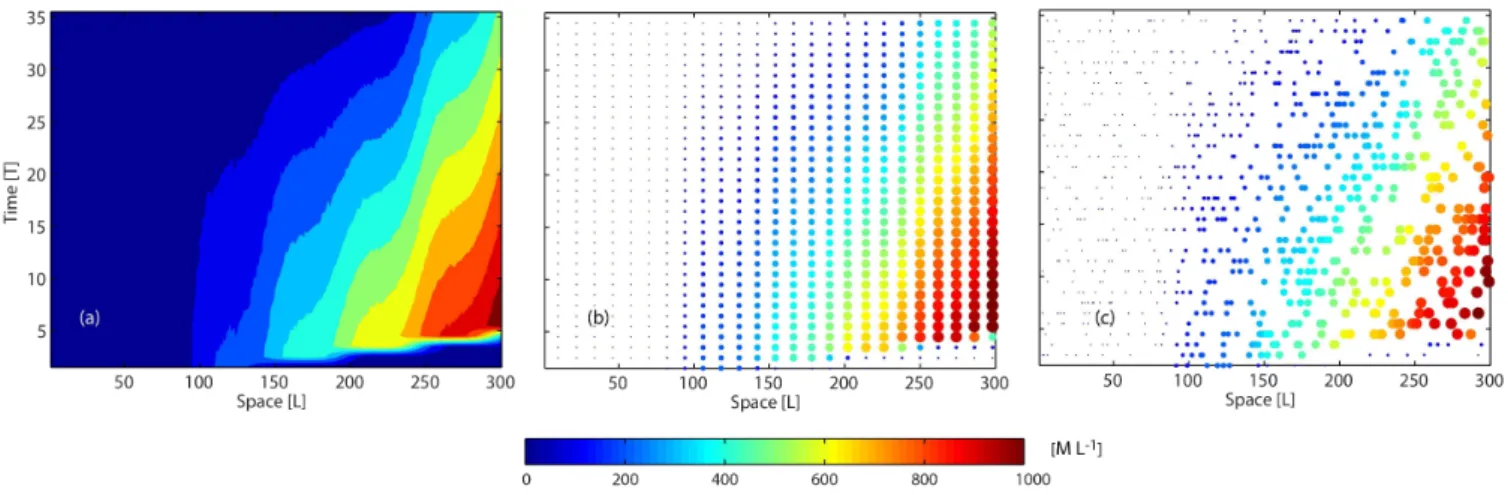
Fig. 1. (a)Spatiotemporal variability of the tracer flux. (b)True flux profile for a particular time period corresponding to the dashed white
line in(a). Also shown in(b)is the prior estimate of the tracer flux profile with its ±2σQprior uncertainty (dashed lines).
generic. Both the length of the 1-D domain and the time pe-riod of the experiment are arbitrarily discretized. The param-eters for the experiment are: the grid size 1x= 1 [L], the domain lengthx= 300 [L], the time step of release 1t= 1 [T], the total number of time periods over which the tracer flux is releasedt= 35 [T], the longitudinal dispersion coeffi-cientDL= 2.0 [L2T−1], and the advection velocityv= 50.0 [L T−1].
The tracer fluxs[M L−1T−1] that is released (Fig. 1a) is modeled as
s(xr,tr)=0.25(36−tr)exp "
−(xr−70) 2
200 #
+exp "
−(xr−130) 2
50 #
+exp
"
−(xr−150)
2
50
#
+0.25(tr)exp
"
−(xr−220)
2
200
#
, (2) where xr represents the locations along the 1-D domain (xr= 1, 2, 3,. . . , 299, 300 [L]) over which the tracer flux is released continuously over 35 fixed intervals (tr= 1, 2, 3,. . . , 34, 35 [T]), with each interval being a duration of 1 [T]. Equation 2 is designed to model two large peaks with fluctu-ating amplitudes (Fig. 1b) between 50 and 100 [L] and be-tween 200 and 250 [L], as well as a smaller consistent dou-ble peak (Fig. 1b) between 100 and 200 [L]. Even though the spatial tracer flux profiles are different for each time pe-riod, the spatially averaged flux has a constant value of 0.84 [M L−1T−1] across all time periods. Note that the true tracer fluxsis used only for simulating the observations and is later assumed unknown throughout the analysis.
The tracer is sampled at locations xo (xo= 1, 2,. . . , 299, 300 [L]) for 35 consecutive time periods (to= 1.5, 2.5,. . . , 34.5, 35.5 [T]) to obtain the observational data setz [M L−1], such that the observation times are offset from the release times. The initial random error with a prespecified
variance (10 [M2L−2]) is added to the tracer observations to simulate measurement, transport, aggregation, and represen-tation errors. Later in the study, different configurations ofxo and error variances variances (σR2) are prescribed to test the
impact of factors.
The tracer observations (z) and the tracer fluxes (s) are related in the following fashion:
z=Hs+ν,whereν ∼N (0,R) , (3)
whereHis the sensitivity matrix that is generated using a 1-D tracer transport model as
Ho,r=
1 2
erfc
(xo−xr)−vto 2√DLto
−erfc
(xo−xr)−v (to−tr)
2√DL(to−tr)
, (4) wherexrandtrare the tracer flux release locations and times, xo and to are the tracer observation locations and times,
erfcrepresents the complementary error function. The tracer transport model embedded in Eq. (4) assumes conservation of mass and is based on a well-known one-dimensional an-alytical solution for a conservative tracer with a continuous source under steady-state conditions (e.g., Ogata and Banks, 1961; Runkel, 1996).
Fig. 2.Observations of the tracer obtained from the three network configurations – REF(a), HM(b), and HT(c). Note that going from the REF to the HM and the HT networks, the total number of observations decreases by a factor of 12, whereas in going from the HM to the HT network, the observational network becomes more heterogeneous in space and time.
allows nearly all of the flux influence on observations to be represented within the DA approaches. The finite lag win-dow also recognizes the operational limitations associated with the implementation of DA approaches in a real-world setting, and we foresee this as a realistic scenario for future global inversions (see Appendix A for a more detailed dis-cussion).
The final piece of information necessary for setting up the inverse problem is the prior estimate (sb) of the tracer flux and its error characteristics (Fig. 1b).sbis chosen here to be constant across all time periods:
sb(xr,tr)=exp
"
−(xr−150) 2
2000
#
. (5)
Its error covariance matrix Qb is based on an exponential decay model in space, with a correlation length (3lQ) of 90
[L] and variance (σQ2)of 3 [M2L−2T−2].
The 1-D framework was designed to capture most of the characteristic features of the CO2flux estimation problem. For a real CO2 inversion, units are most typically [µmol (m2s)−1] for s andσQ, [ppm] for zand σR, [ppm µmol−1
(m2s−1)] forH, and [km] forlQ.
2.3 Experiments
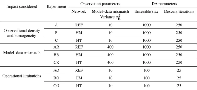
Experiments are designed to explore the impact of three fac-tors on the ability of the DA approaches to solve the inverse problem: (a) the observational density and homogeneity, (b) the model–data mismatch covariance, and (c) the operational constraints of the DA system (i.e., ensemble size, number of descent iterations). In all the experiments, the size of the state vector or the total number of fluxes to be inferred is 10 500×1 (i.e., 300 locations×35 times).
The first set of experiments (Table 1 – experiments A through C) aims to investigate the effect of the density and
spatiotemporal homogeneity of the observational network. Three different observational networks are designed (Fig. 2). In the first network configuration (denoted as REF – “ref-erence observational set” as outlined in Sect. 2.2), observa-tions are obtained throughout the domain (xo= 1, 2,. . . , 299, 300 [L]) and for all 35 measurement times (to= 1.5, 2.5,. . . , 34.5, 35.5 [T]) (Fig. 2a). The total number of observations available is thus 10 500 (i.e., 300 locations×35 times). In the second network configuration (denoted as HM – “homo-geneous”), observations are obtained at 25 equally spaced locations within the 1-D domain (xo= 10, 22, 34. . . , 298 [L]) for all 35 time periods (to= 1.5, 2.5,. . . , 34.5, 35.5 [T]) (Fig. 2b). The total number of observations is thus reduced to 875 (i.e., 25 locations×35 times). In the final configu-ration (denoted as HT – “heterogeneous”), observations are taken at 25 randomly selected locations for each measure-ment time (to= 1.5, 2.5,. . . , 34.5, 35.5 [T]) (Fig. 2c), and these locations vary from one time to the next. Similarly to HM, the total number of observations in HT is 875 (i.e., 25 locations×35 times), but the observations are neither uni-form in space nor consistent in time. Note that unlike REF, both HM and HT represent underdetermined inversion prob-lems where the total number of observations is substantially lower than the number of unknowns in the state space to be estimated. In reality, the HT network configuration scheme is the closest to current CO2monitoring networks where dif-ferent monitoring locations (ground based or remote sensing) can come online and go offline over different periods.
Table 1.Summary of the experiments outlined in Sect. 2.3. The following parameters are held constant for all the experiments in this study:
sb(Eq. 5), 3lQ= 90 [L] andσQ2= 3 [M2L−2T−2].
Impact considered Experiment Observation parameters DA parameters
Network Model–data mismatch Ensemble size Descent iterations
VarianceσR2
Observational density
A REF 10 1000 250
and homogeneity B HM 10 1000 250
C HT 10 1000 250
Model–data mismatch
AR REF 400 1000 250
BR HM 400 1000 250
CR HT 400 1000 250
Operational limitations
AO REF 10 100 25
BO HM 10 100 25
CO HT 10 100 25
have no spatial or temporal correlation. Finally, all three ap-proaches use the same numerical realization of errors, thus ensuring that they are solving the same inverse problem.
The second set of experiments (Table 1 – experiments AR through CR) examines the effect of the model–data mismatch variance on the best estimates and their associated uncertain-ties. For all the network configurations, the variance of the random errors is increased to 400 [M2L−2] with the diag-onal values of the model–data mismatch covariance matrix
Rincreased accordingly. All other parameters are kept the same as in the first set of experiments.
The third set of experiments (Table 1 – experiments AO through CO) explores the impact of operational constraints, which are always an important consideration in implement-ing a DA system. To minimize numerical approximations and avoid sampling or convergence errors, the ensemble size (for EnSRF) and the number of descent iterations (for 4D-VAR) for the first two sets of experiments (Table 1 – experiments A–C and experiments AR–CR) are set to 1000 and 250, re-spectively. The number of descent iterations is prescribed to be lower than the number of ensemble members, keeping in mind that 4D-VAR typically requires more model integra-tions (i.e., both forward and adjoint model run) than EnSRF. Given that it is not feasible to either run a large number of ensemble members or specify a large number of descent it-erations for real atmospheric applications, these numbers are reduced to 100 ensemble members for EnSRF and 25 de-scent iterations for 4D-VAR in the third set of experiments. The noise added to the observations is kept the same as in the first set of experiments, namely 10 [M2L−2], to allow for a direct comparison with experiments A–C.
3 Results
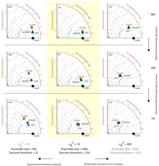
In the sections that follow, results from the nine experiments are interpreted at both the native and aggregated spatial scales, and estimates from the EnSRF and the 4D-VAR ap-proaches are compared both to the truth and to the estimates from the BIM approach. Taylor diagrams (Taylor, 2001) are used to assess the root-mean-square difference (RMSD) and the correlation coefficient (CC) between the flux estimates and the truth, as well as the standard deviation (SD) of the flux estimates and the truth. These metrics are calculated across 30 time periods (tr= 6, 7,. . . , 34, 35 [T]) to be rep-resentative of the overall experiment after discarding the first five time periods as spin-up.
3.1 Impact of observational density and homogeneity
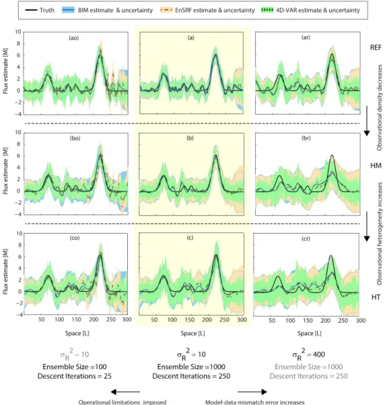
For the REF network (experiment A), all three approaches perform well in recovering the true flux (e.g., Fig. 3a), and in fitting the observations within the specified model–data mismatch errors (results not shown). For the sample time period presented in Fig. 3a, both the 4D-VAR and the En-SRF estimates capture the flux profile, including its large and small peaks. These results are typical of the performance of the three approaches across other estimation times. The performance across the full examined time period is summa-rized in Fig. 4a, where all three approaches show a high CC (∼0.97), low RMSD (∼0.3 [M L−1T−1]), and standard de-viations (∼1.5 [M L−1T−1]) that are similar to that of the true fluxes.
Fig. 3.Example of estimated tracer fluxes (lines) and associated±2σˆsuncertainties (shaded areas) for the different approaches assessed in this study. All values are shown for the 25th time period, which is representative of the observed performance over other time periods. The panel titles correspond to the different experiments outlined in Table 1.
double peak around 100–200 [L], and the Taylor diagrams in Fig. 4b and c show a corresponding drop in CC and an in-crease in RMSD. In general, for observations with spatially uncorrelated model–data mismatch errors such as those used here, decreasing the observational density is expected to de-crease the analysis accuracy. The response of the two DA ap-proaches mirrors the BIM approach in such cases, including the inference of an incorrect flux pattern for the HT network around 100 [L] in Fig. 3c. This result indicates that in the ab-sence of operational constraints, best estimates from the DA approaches are consistent with the BIM estimate even for an underdetermined inverse problem.
In terms of the recovered posterior uncertainty estimates, the EnSRF uncertainty estimates are more consistent with the BIM uncertainty estimates relative to 4D-VAR (Fig. 3a– c). For the REF observational configuration, the average
ra-tios of the predicted posterior uncertainty of the individual flux estimates in EnSRF (σˆsEnSRF) and 4D-VAR (σsˆ4D−VAR)to those from BIM (σsˆBIM)are approximately 0.98 and 0.84, re-spectively; that is, on average, EnSRF and 4D-VAR under-estimate the posterior uncertainties by 2 and 16 %, respec-tively, relative to BIM (Fig. 5a). As the observational density changes, EnSRF overestimates the uncertainty by 2 and 6 % for HM and HT, respectively, while 4D-VAR underestimates the uncertainty substantially, by 22 and 18 %, respectively (Fig. 5b, c). For all cases, the 4D-VAR uncertainties for indi-vidual locations/times over- or underestimates the BIM esti-mates even more substantially than evidenced by the average statistics, however, as seen by the spread in the histograms in Fig. 5.
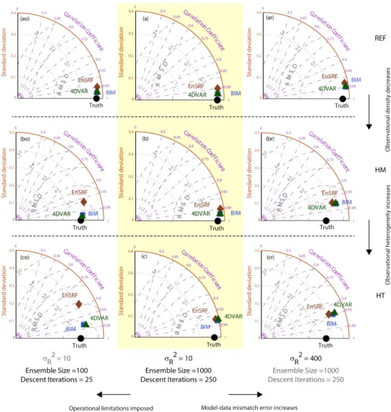
Fig. 4.Performance of the BIM, the EnSRF, and the 4D-VAR approaches for the different experiments outlined in Table 1. For each experi-ment, statistics are calculated between the estimates and the true fluxes across all locations and all 30 time periods and are represented on a Taylor diagram. For each Taylor diagram, the true flux is represented by a point along the abscissa corresponding to the standard deviation of the true fluxes (“Truth”). All other points (“BIM”, “EnSRF”, “4D-VAR”), which represent the estimated fluxes, are positioned such that their standard deviation is the radial distance from the origin, the correlation coefficient between the estimates and the truth is the cosine of the azimuthal angle, and the root-mean-square difference (RMSD) between the estimates and the truth is the distance to the observed point. In the limit of perfect agreement, these other points would coincide with “Truth” (i.e., RMSD = 0, CC = 1, and SD of the estimates would be the same as that of the truth).
model, there is little source of variability for the ensemble to maintain a consistent spread. As observations are assimi-lated, the ensemble members tend to collapse to the ensem-ble mean and the adaptive inflation (see Appendix A.3) has to compensate for this degeneracy by inflating the ensem-ble spread. In the HT case, however, the inflation technique has a delayed response in adjusting to the heterogeneity in the observational network, as different observation locations come into and out of the network. For the adaptive inflation component to function well, we find it beneficial to have a consistent set of observations to maintain a reasonable en-semble spread (e.g., Chatterjee et al., 2012). It is worthwhile
to mention here that the magnitudes of the inflation factors are very small in experiments A–C. This is not surprising given that a large number of ensemble members have been specified and the sampling error is hence quite low.
Fig. 5.Histogram showing the ratio of the estimated posterior uncertainties from the EnSRF (σsˆ
EnSRF) and the 4D-VAR (σsˆ4D-VAR) approaches
to the posterior uncertainties from the BIM (σsˆBIM) approach. The ratios are calculated for each estimated flux time/location over all 30 time
periods to be representative of the overall experiments outlined in Table 1. In the ideal case – that is, if the posterior uncertainty from a DA approach is equal to the posterior uncertainty from BIM – the histogram would be a single line centered around 1.
test in which the total number of perturbations is increased (or decreased) indicated that the heterogeneity of the uncer-tainty estimates obtained via the Monte Carlo technique de-creased (or inde-creased) correspondingly. When averaged over all the time periods (Fig. 5a–c), the posterior uncertainty esti-mates clearly underestimate the BIM uncertainty. Even then, the large spread in the histograms shown in Fig. 5a–c rein-forces our earlier conclusions that the uncertainty estimates for individual fluxes over/underestimate the BIM uncertainty estimates substantially.
Overall, we find that both 4D-VAR and EnSRF can repro-duce the performance of BIM in terms of the best estimates of the fluxes for all three observational network configura-tions. Even though small discrepancies are noticeable, the impact of a sparse and/or heterogeneous observational
net-work is similar for the DA approaches compared to the BIM approach. Both the DA approaches have some difficulty in reproducing the BIM posterior uncertainty estimates, albeit for different reasons. In the absence of any operational con-straints, however, EnSRF provides more realistic and useful uncertainty bounds than 4D-VAR.
3.2 Impact of model–data mismatch covariance
experiments, EnSRF and 4D-VAR best estimates respond similarly to BIM when the model–data mismatch covariance changes, and both the approaches track the BIM best esti-mates quite well for all the three experiments. Figure 4ar–cr confirm that the best estimates from all the three approaches have a lower CC, higher RMSD, and lower SD when com-pared to Fig. 4a–c.
The standard deviation of the flux estimates change con-siderably between Fig. 4ar (∼1.45–1.5 [M L−1T−1]) and 4cr (∼0.94–1.00 [M L−1T−1]) for the three approaches. In-creasing theσR2to 400 [M2L−2] results in the analysis reject-ing the information from the observations and givreject-ing more weight to the prior, yielding overly smooth a posteriori es-timates. A typical example of this is seen by comparing the estimated peak around 50–100 [L] in Fig. 3c and cr. Esti-mates in both these panels are based on the same observa-tional network but the estimates in Fig. 3cr do not capture the amplitude of the two large peaks in the true flux signal.
For experiments AR–CR, the posterior uncertainty esti-mates for all the three approaches are higher compared to experiments A–C, as expected due to the higher prescribed model–data mismatch error. Similarly to experiments A– C, the 4D-VAR uncertainty estimates for individual loca-tions/times are too variable relative to BIM (Fig. 5). Aver-aged over time and space, the 4D-VAR uncertainty estimates underestimate the BIM uncertainty estimates by approxi-mately 25 % (Fig. 5ar–cr). Thus, even though the 4D-VAR uncertainty estimates for experiments AR–CR are higher than the corresponding uncertainty estimates for experiments A–C, they fail to capture the full magnitude of the BIM un-certainty estimates. This makes intuitive sense due to the indirect approach adopted for generating the 4D-VAR un-certainty estimates. Conversely, as the observational net-work becomes sparser and more heterogeneous, the EnSRF slightly overestimates the BIM average uncertainties by 3 % (HM; Fig. 5br) and 5 % (HT; Fig. 5cr), while it underesti-mates the uncertainty by only 1 % for the reference network (Fig. 5ar). The EnSRF uncertainty estimates for individual locations/times are more closely distributed around the BIM estimates (Fig. 5). The better performance of EnSRF in terms of the uncertainty estimation can be directly related to the en-semble spread. Relative to experiments A–C, when the pre-scribed model–data mismatch error is high in experiments AR–CR, the initial ensemble spread is reduced by a lower amount as observations are now being given less weight and hence have lower impact on the ensemble spread. Con-sequently, the ensemble members maintain a large spread throughout the analysis and results in large posterior uncer-tainty estimates that are more realistic relative to 4D-VAR.
Experiments AR–CR reconfirm that in the absence of op-erational limitations, an increase (or decrease) in the model– data mismatch covariance does not affect the ability of the DA approaches to reproduce the BIM best estimates. Similar to experiments A–C, in terms of the posterior uncertainty es-timates, however, (a) both the DA approaches are less skilled
at reproducing the uncertainty estimates from BIM, and (b) the uncertainty estimates from 4D-VAR severely underesti-mate the BIM uncertainty estiunderesti-mates and are less realistic than the EnSRF uncertainty estimates.
3.3 Impact of operational constraints
Operational constraints hinder the performance of the DA ap-proaches, and the impact is further intensified as the obser-vational network becomes more heterogeneous.
For 4D-VAR, an inadequate number of iterations may lead to a failure to find the minimum of the quadratic objective function (convergence results not shown here). When the ob-servational network is heterogeneous, the minimization has even more difficulty in finding the path towards the mini-mum. Thus, comparing Fig. 4ao–co, the 4D-VAR estimates diverge from the BIM estimates for the HT network configu-ration. In general, we find that for the HT network, 4D-VAR needs approximately 50 iterations to converge completely for the case studies presented here. Conversely, for the REF and the HM network, 4D-VAR requires only approximately 20 to 30 iterations to reach full convergence. For all the three experiments, however, the value of the objective function is reduced relative to that for the prior fluxes, indicating an im-provement over the prior estimates. As pointed out by Rö-denbeck (2005), the minimization determines the large-scale gradient in the initial iterations, while in subsequent itera-tions fine-scale tuning is performed to capture the optimum. By artificially limiting the number of iterations in experi-ments AO–CO, the ability of 4D-VAR to make small-scale adjustments is hindered, which manifests itself clearly in ex-periment CO (panel co in Figs. 3, 4 and 5).
from EnSRF are still closer to the BIM uncertainty estimates, being within 10 % of the averaged BIM uncertainties for ex-periments AO, BO, and CO, whereas the average 4D-VAR uncertainties underestimate the BIM uncertainties by up to 25 %. The degradation in the uncertainty estimates provided by 4D-VAR and EnSRF is due to different reasons. While for EnSRF the large sampling error plays a dominant role, for 4D-VAR the perturbations in the Monte Carlo technique are unable to capture the true range of the posterior uncertainties. The impact for 4D-VAR is accentuated for experiments BO and CO, where the sparse network exacerbates the need for more iterations to reach convergence.
An important caveat here is that the results for both the DA approaches could potentially be improved through fur-ther tuning of each algorithm. For example, the implementa-tion of more sophisticated algorithms to precondiimplementa-tion and ob-tain faster convergence, or stronger localization schemes to dampen the spurious noise in the ensemble members, might provide slightly different responses and reduce the error in-curred due to the numerical approximations. In spite of hav-ing state-of-the-art algorithms, however, once the underlyhav-ing numerical approximations come into play, (a) EnSRF fails to reproduce the BIM best estimates, with the EnSRF per-formance decreasing as the observational network becomes sparser and more heterogeneous, and (b) 4D-VAR also fails to reproduce the BIM best estimates when the observational network is heterogeneous but still performs better than En-SRF. The better performance of 4D-VAR in terms of the flux estimates is offset by the fact that EnSRF provides more re-alistic uncertainty bounds on the recovered flux estimates.
The DA approaches are particularly sensitive to the infor-mation flow from the observations because of the lack of an explicit dynamical model. As discussed in Sect. 1, a dynam-ical model adds to the information content of the system, al-beit at the cost of additional model errors that must be taken into account. Identifying/developing an appropriate dynami-cal model relevant to the CO2flux estimation problem, and subsequently repeating experiments such as those presented here, may further inform the assessment of the interplay be-tween the operational constraints and the observational net-work.
flux and the flux estimates are aggregated over each of these areas and examined across time. This is qualitatively anal-ogous to aggregating fluxes a posteriori to “large regions” (e.g., biomes, continents) within the inversion domain. Be-cause the true flux differs between these two subregions, and these differences themselves vary in time, it is possible to ex-amine the ability of the various approaches to capture these spatiotemporal variations. Figure 6 presents the comparison at the aggregated scales in the form of a Taylor diagram. For all the 9 experiments, 4D-VAR is able to match the tempo-ral variation of the spatially aggregated BIM estimates bet-ter than EnSRF. Even when the number of descent ibet-terations is reduced (Fig. 6ao–co), the differences between the BIM and the 4D-VAR best estimates are negligible at the exam-ined spatially aggregated scales. Comparing Figs. 4co and 6co demonstrates that the differences observed at fine scales are substantially reduced when aggregating the estimates to a coarser resolution.
Because there is no explicit dynamical model to evolve the information between assimilation time periods, the EnSRF estimates are always contaminated with small-scale sampling errors, but these errors partially cancel out when the esti-mates are spatially aggregated. Overall, the EnSRF estiesti-mates still, however, exhibit more spurious variability relative to the 4D-VAR estimates. Especially when the number of en-semble members is reduced (Fig. 6ao–co), both the sampling error as well as the observational density and heterogeneity start to play a role, leading to less reliable estimates at ag-gregated scales. For example, in Fig. 6ao and 6co, the CC between the spatially aggregated EnSRF and the true flux es-timates drops from 0.99 to 0.90, and the RMSD increases from 0.03 to 0.21 [M L−1T−1]. The standard deviation of these spatially aggregated EnSRF estimates also increases from 0.37 to 0.40 [M L−1T−1], leading to an overestima-tion relative to the true flux, which has a standard deviaoverestima-tion of 0.36 [M L−1T−1].
Fig. 6.Performance of BIM, EnSRF, and 4D-VAR at spatially aggregated scales for the different experiments outlined in Table 1. The details of the plot are as described in the caption of Fig. 4.
and lower RMSD than the corresponding estimates at the fine scale (Fig. 4co). This is encouraging from the perspective of a real CO2flux estimation problem, as it implies that the DA approaches may provide reliable flux estimates at aggregated scales, even under circumstances when their performance at fine scales is compromised.
4 Discussion
Overall, the choice between 4D-VAR and EnSRF approaches for the CO2 flux estimation problem should be based on the carbon science questions being targeted, as well as the tradeoff between the impact of incomplete convergence of the minimization algorithm (for 4D-VAR) and the impact of sampling error (for EnSRF) on the estimated fluxes and their uncertainties.
subjective. Experiments in this study show, for example, that the localization length scale is dependent on both the ensem-ble size and the observational density. Will increasing vol-umes of observations push us towards specifying shorter lo-calization length scales? If so, what is the limit beyond which decreasing the localization length scale may actually degrade the analysis? It is necessary to identify more rigorously a ba-sis for selecting the localization parameters (e.g., Anderson, 2012) or adaptive approaches that may be less sensitive to variations in the observational network.
One critical requirement of an inverse problem is to ob-tain reliable second-order statistical moments for the esti-mated system states. Even though we have demonstrated that posterior error statistics can be obtained for both EnSRF (directly) and 4D-VAR (indirectly via a Monte Carlo tech-nique), the EnSRF uncertainty estimates reproduce the BIM uncertainty estimates consistently better. The indirect tech-niques necessary for obtaining posterior error statistics for 4D-VAR has important caveats, as demonstrated by the large over/underestimation of uncertainties for individual flux lo-cations and times, as well as the underestimation of the pos-terior uncertainties relative to BIM when averaged across all locations and times. Therefore, EnSRF is more desirable for attribution purposes, wherein source–sink estimates with re-alistic confidence bounds can be used to gain a better un-derstanding of the mechanistic processes driving the carbon cycle or to reconcile estimates from top-down and bottom-up approaches.
With both 4D-VAR and EnSRF, there is a direct trade-off between computational savings and estimation accuracy, which is intensified when solving an underdetermined prob-lem with a heterogeneous observational network. For large-scale flux estimation problems, operational constraints will always exist, as will scarce and inconsistent observations, transport model biases and uncertainties (thus further lim-iting the use of available observations), etc. The HT scheme with a limited number of ensemble members/descent itera-tions (panel co in Figs. 3, 4 and 5) serves as the closest ana-logue to a real inversion problem. Even if we account for the increase in remote-sensing measurements of CO2, the obser-vational network is going to be a complex hybrid between the REF and the HT scheme. In this scenario, the accuracy
mates of analysis error that are more realistic than those op-erationally feasible for 4D-VAR. The relative performance of 4D-VAR and EnSRF best estimates, when a large and homo-geneous set of observations is available, is consistent with the conclusions obtained from intercomparison studies car-ried out by other DA communities. The sensitivity of the ap-proaches to the observational scheme in the absence of an explicit dynamical model, and specifically for solving an un-derdetermined inverse problem, however, had not previously been thoroughly explored. Beyond CO2source–sink estima-tion problems, the conclusions of this study are therefore also relevant to other DA problems where a dynamical model is lacking.
The sensitivity experiments demonstrate that when a large number of ensemble members or descent iterations is speci-fied, the best estimates obtained from state-of-the-art imple-mentations of the 4D-VAR and the EnSRF approaches are similar to those from BIM, irrespective of the observational characteristics. Even under these optimal conditions, how-ever, the uncertainty estimates from 4D-VAR are unable to reproduce those from BIM. When operational constraints are imposed, both the characteristics of the observational net-work and the numerical approximations play a greater role in differentiating the performance of the two DA approaches. Because such operational constraints are always present for real CO2source–sink estimation problems, the choice of an approach should be based on (a) the carbon science ques-tions being targeted (i.e., whether the science calls only for best estimates of fluxes, or for flux estimates with realistic uncertainties) and (b) the inversion conditions under which they are being applied (i.e., characteristics of the observa-tional network, such as data density and heterogeneity).
Appendix A
Estimation methods for solving the inverse problem A1 Batch inverse modeling (BIM)
In the BIM approach (e.g., Enting, 2002), the analytical solution for the a posteriori estimate and the associated covariances of the objective function (Eq. 1) are given by ˆ
sa=sb+Kz−Hsb
, (A1)
Qa=(I−KH)Qb, (A2)
K=QbHTHQbHT+R−
1
. (A3)
wheresˆa is the posterior best estimate of the state and Qa
is the a posteriori covariance of the recovered best estimate. The diagonal elements of Qa represent the predicted er-ror variance (σsˆ2) of individual elements insˆa. As stated in Sect. 1, for CO2inversion studies, the generation of the ma-trix H requires an atmospheric transport model to be run either once per estimated element of the state vector, or once per observation. The large number of model runs ulti-mately makes the BIM approach computationally intractable for solving very large-scale problems.
A2 Four-dimensional variational (4D-VAR)
In 4D-VAR, the fluxessˆa that minimize the objective func-tion in Eq. (1) are sought iteratively by minimizing the misfit between a feasible state trajectory and the observations that are available over a given assimilation window. The over-all approximation lies in the fact that the minimization can be stopped by artificially limiting the number of iterations or by requiring that the norm of the gradient decreases by a predefined amount during each iteration. Most minimization schemes rely on the availability of the gradient of the objec-tive function with respect to the state (or control vector in 4D-VAR terms),
∇J (s)=Qb−1hs−sb
i
+HTR−1[z−h(s)]. (A4) Instead of analytically calculating the gradient, the adjoint of the forward transport model is used to compute the termσ2 ˆ s directly, which is then added toˆsin Eq. (A4) above. While a variety of minimization schemes may be used (e.g., conju-gate gradient or BFGS, e.g., Nocedal and Wright, 2006), in this study, we use a Lanczos minimizer algorithm (e.g., No-cedal and Wright, 2006), which produces similar results as the conjugate-gradient technique in terms of the reduction of the cost function and gradient norm but converges substan-tially faster. Additionally, a new variable (4) is defined to precondition the minimization as
4=Qb−
1 2
s, (A5)
where 4 now becomes the control variable with respect to which the objective function is minimized instead of s directly. The optimal preconditioning matrix to reduce the number of iterations required to solve the minimization prob-lem is the inverse Hessian (Axelsson and Barker, 2001). For a real high-dimensional CO2inversion problem, however, the size and structure of the prior covariance matrix may consti-tute a significant impediment for calculating the inverse Hes-sian. Any algebraic manipulations, such as taking inverses or calculating the square roots for preconditioning purposes, become operationally cumbersome and thus matrix manipu-lation techniques (e.g., Yadav and Michalak, 2013) are nec-essary to sidestep these operational challenges.
The main caveat with the variational approaches, such as 4D-VAR, is that a direct estimate of the analysis error is not available (no clear analogue of Eq. A2). Mathematically this can be obtained from the inverse of the Hessian (e.g., Le Dimet et al., 2002; Rödenbeck, 2005; Meirink et al., 2008) but operational challenges restrict the calculation and stor-age of the Hessian for high-dimensional problems. Recent applications of 4D-VAR for NWP problems have shown that computationally efficient alternatives do exist (e.g., Cheng et al., 2010; Gejadze et al., 2013). Although some of these tech-niques are more suited for nonlinear problems (e.g., Gejadze et al., 2013), they retain potential applicability to the CO2 flux estimation problem as well. In this study, we use a Monte Carlo technique (e.g., Chevallier et al., 2007) where both the observations and the prior are perturbed multiple times with the prespecified model–data mismatch error statistics and prior error statistics, respectively.
4D-VAR is implemented with successive overlapping win-dows to (a) account for the long residence times of CO2 in the atmosphere and (b) to avoid the operational cost associ-ated with calculating the inverse of the full prior covariance matrixQbin Eqs. (A4) and (A5). In order to determine the length of the moving window, however, one needs to keep in mind two primary factors: (a) observations typically in-form fluxes over a finite period of time (e.g., 4- to 6-month time frame based on the analysis reported in Bruhwiler et al., 2005), and (b) temporal correlation in the prior flux errors (e.g., for the prior land flux errors Chevallier et al. (2012) has suggested the temporal correlation to be strongly positive for lags<85 days and mildly positive for lags>275 days). Given a sufficiently long window the 4D-VAR approach us-ing a movus-ing window will emulate the 4D-VAR approach using a single window, while at the same time providing sub-stantial computational savings. In the absence of a dynami-cal model, this implementation of 4D-VAR becomes similar to the FGAT-3DVAR (Massart et al., 2010) variant occasion-ally used within the NWP community.
A3 Ensemble square root filter (EnSRF)
ter (Whitaker and Hamill, 2002) implemented in a fixed-lag smoother form (e.g., Whitaker and Compo, 2002; Chatter-jee et al., 2012). Similarly to an ensemble square root filter, the ensemble smoother uses Monte Carlo estimates of the er-ror covariances to compute a Kalman smoother gain matrix. This is applied iteratively to a time series of observations, where the analysis at the first time step is equivalent to an ensemble square root filter analysis as it only utilizes obser-vations taken up to and including the analysis time. All sub-sequent time steps utilize observations taken a number of ob-serving times past the analysis time. The localization scheme (i.e., to cut down spurious noise in the ensemble members) is based on Houtekamer and Mitchell (2001) using a fifth-order Gaspari–Cohn function (Gaspari and Cohn, 1999), while the adaptive inflation algorithm (i.e., to counter spurious vari-ance deficiency among the ensemble members) is based on Anderson (2009). Implementation of these algorithms within an ensemble smoother framework is described in further de-tail in Chatterjee et al. (2012). Despite these ancillary algo-rithms, the overall implementation of EnSRF is quite simple and computationally efficient.
A4 Sensitivity tests and additional approaches considered
The setup of 4D-VAR (with overlapping time windows) and EnSRF (expressed as a fixed-lag smoother) reflect state-of-the-art implementations of these two DA approaches, keep-ing in mind the nature of the atmospheric CO2process, the fact that CO2observations only provide significant informa-tion about fluxes over a finite preceding time window, and the operational constraints for estimating CO2fluxes at high spatiotemporal scales (e.g., spatial ∼1◦, temporal ∼daily). Note that we have implemented both approaches with a sin-gle long window as a sensitivity test. Other than an increase in the computational cost, the conclusions regarding the per-formance of the approaches relative to the BIM approach are the same as those reported in the manuscript. We have also tested other varieties of the ensemble filter (EnKF with perturbed observations (Evensen, 2003) and the variational approach (PSAS; Courtier, 1997) and found that the over-all conclusions from the presented experiments remain
con-by the University Corporation for Atmospheric Research.
Edited by: M. Heimann
References
Anderson, J. L.: Spatially and temporally varying adaptive covari-ance inflation for ensemble filters, Tellus A – Dyn. Meteorol. Oceanogr., 61, 72–83, doi:10.1111/j.1600-0870.2008.00361.x, 2009.
Anderson, J. L.: Localization and Sampling Error Correction in En-semble Kalman Filter Data Assimilation, Mon. Weather Rev., 140, 2359–2371, doi:10.1175/mwr-d-11-00013.1, 2012. Axelsson, O. and Barker, V. A.: Finite-Element Solution of
Boundary-value Problems. Theory and Computation, vol. 35 of Classics in Applied Mathematics, SIAM, Philadelphia, PA, 432 pp. (Reprint of the 1984 original), 2001.
Baker, D. F., Doney, S. C., and Schimel, D. S.: Variational data
assimilation for atmospheric CO2, Tellus Series B-Chemical
and Physical Meteorology, 58, 359-365, doi:10.1111/j.1600-0889.2006.00218.x, 2006.
Bauer, P., Lopez, P., Benedetti, A., Salmond, D., and Moreau,
E.: Implementation of 1D+4D-Var assimilation of
precipitation-affected microwave radiances at ECMWF. I: 1 D-Var, Q. J. Roy. Meteorol. Soc., 132, 2307–2332, doi:10.1256/qj.05.189, 2006. Bengtsson, T., Snyder, C., and Nychka, D.: Toward a nonlinear
en-semble filter for high-dimensional systems, J. Geophys. Res., 108, 8775–8785, doi:10.1029/2002JD002900, 2003.
Brankart, J.-M., Ubelmann, C., Testut, C.-E., Cosme, E., Brasseur, P., and Verron, J.: Efficient parameterization of the observation error covariance matrix for square root or ensemble Kalman fil-ters: application to ocean altimetry, Mon. Weather Rev., 137, 1908–1927, doi:10.1175/2008MWR2693.1, 2009.
Bruhwiler, L. M. P., Michalak, A. M., Peters, W., Baker, D. F., and Tans, P.: An improved Kalman Smoother for atmospheric inver-sions, Atmos. Chem. Phys., 5, 2691–2702, doi:10.5194/acp-5-2691-2005, 2005.
Buehner, M., Houtekamer, P. L., Charette, C., Mitchell, H. L., and He, B.: Intercomparison of Variational Data Assimilation and the Ensemble Kalman Filter for Global Deterministic NWP. Part I: Description and Single-Observation Experiments, Mon. Weather Rev., 138, 1550–1566, 2010a.
Ensemble Kalman Filter for Global Deterministic NWP. Part II: One-Month Experiments with Real Observations, Mon. Weather Rev., 138, 1567–1586, 2010b.
Carmichael, G. R., Sandu, A., Chai, T., Daescu, D. N., Con-stantinescu, E. M., Tang, Y.: Predicting Air Quality: Im-provements through advanced methods to integrate mod-els and measurements, J. Comput. Phys., 227, 3540–3571, doi:10.1016/j.jcp.2007.02.024, 2008.
Caya, A., Sun, J., and Snyder, C.: A comparison between the 4DVAR and the ensemble Kalman filter techniques for radar data assimilation, Mon. Weather Rev., 133, 3081–3094, 2005. Chatterjee, A., Michalak, A. M., Anderson, J. L., Mueller, K. L.,
and Yadav, V.: Towards reliable ensemble Kalman filter
esti-mates of CO2fluxes, J. Geophys. Res.-Atmos., 117, D22306,
doi:10.1029/2012JD018176, 2012.
Cheng, H. Y., Jardak, M., Alexe, M., and Sandu, A.: A hybrid ap-proach to estimating error covariances in variational data assim-ilation, Tellus A – Dyn. Meteorol. Oceanogr., 62A, 288–297, doi:10.1111/j.1600-0870.2010.00442.x, 2010.
Chevallier, F., Fisher, M., Peylin, P., Serrar, S., Bousquet, P.,
Breon, F.-M., Chedin, A., and Ciais, P.: Inferring CO2sources
and sinks from satellite observations: Method and applica-tion to TOVS data. J. Geophys. Res.-Atmos., 110, D24309, doi:10.1029/2005JD006390, 2005.
Chevallier, F., Breon, F.-M., and Rayner, P. J.: Contribution of
the Orbiting Carbon Observatory to the estimation of CO2
sources and sinks: Theoretical study in a variational data as-similation framework, J. Geophys. Res.-Atmos., 112, D09307, doi:10.1029/2006JD007375, 2007.
Chevallier, F., Wang, T., Ciais, P., Maignan, F., Bocquet, M., Altaf Arain, M., Cescatti, A., Chen, J., Dolman, A. J., Law, B. E., Margolis, H. A., Montagnani, L., and Moors, E. J.: What eddy-covariance measurements tell us about prior land flux errors
in CO2-flux inversion schemes, Global Biogeochem. Cy., 26,
GB1021, doi:10.1029/2010GB003974, 2012.
Courtier, P.: Dual formulation of four-dimensional variational as-similation, Q. J. Roy. Meteorol. Soc., 123, 2449–2461, 1997. Elbern, H., Strunk, A., and Nieradzik, L.: Inverse Modeling and
Combined State-Source Estimation for Chemical Weather, in Data Assimilation, Making Sense of Observations, edited by: La-hoz, W., Khattatov, B., Menard, R., 491–515, Springer-Verlag Berlin, 2010.
Enting, I. G.: Inverse Problems in Atmospheric Constituent Trans-port. Atmospheric and Space Science Series, 392 pp.,Cambridge University Press, Cambridge, 2002.
Evensen, G.: The Ensemble Kalman Filter: theoretical formulation and practical implementation. Ocean Dynamics, 53, 343–367, 2003.
Eyre, J. R., Kelly, G. A., McNally, A. P., Andersson, E., and Pers-son, A.: Assimilation of TOVS radiance information through one-dimensional variational analysis, Q. J. Roy. Meteorol. Soc., 119, 1427–1463, doi:10.1002/qj.49711951411, 1993.
Feng, L., Palmer, P. I., Bösch, H., and Dance, S.: Estimating surface
CO2fluxes from space-borne CO2dry air mole fraction
obser-vations using an ensemble Kalman Filter, Atmos. Chem. Phys., 9, 2619–2633, doi:10.5194/acp-9-2619-2009, 2009.
Fertig, E. J., Harlim, J., and Hunt, B. R.: A comparative study of 4D-VAR and a 4D Ensemble Kalman Filter: perfect model
sim-ulations with Lorenz-96, Tellus A – Dyn. Meteorol. Oceanogr., 59, 96–100, 2007.
Furrer, R. and Bengtsson, T.: Estimation of highdimensional prior and posteriori covariance matrices in Kalman filter variants, J. Multivar. Anal., 98, 227–255, doi:10.1016/j.jmva.2006.08.003, 2007.
Gaspari, G. and Cohn, S. E.: Construction of correlation functions in two and three dimensions, Q. J. Roy. Meteorol. Soc., 125, 723– 757, doi:10.1256/smsqj.55416, 1999.
Gejadze, I. Yu., Shutyaevb, V., and Dimetc, F.-X. L.: Anal-ysis error covariance versus posterior covariance in varia-tional data assimilation. Q.J.R. Meteorol. Soc., 139, 1826–1841, doi:10.1002/qj.2070, 2013.
Gourdji, S. M., Mueller, K. L., Yadav, V., Huntzinger, D. N., Andrews, A. E., Trudeau, M., Petron, G., Nehrkorn, T., Eluszkiewicz, J., Henderson, J., Wen, D., Lin, J., Fischer, M.,
Sweeney, C., and Michalak, A. M.: North American CO2
ex-change: inter-comparison of modeled estimates with results from a fine-scale atmospheric inversion, Biogeosciences, 9, 457–475, doi:10.5194/bg-9-457-2012, 2012.
Haines, K.: Ocean Data Assimilation, in Data Assimilation, Mak-ing Sense of Observations, edited by W. Lahoz, B. Khattatov, R. Menard, 517–547, Springer-Verlag Berlin, 2010.
Houser, P. R., De Lannoy, G. J. M., and Walker, J. P.: Land Surface Data Assimilation, in Data Assimilation, Making Sense of Ob-servations, edited by: Lahoz, W., Khattatov, B., and Menard, R., 549–597, Springer-Verlag Berlin, 2010.
Houtekamer, P. L. and Mitchell, H. L.: A sequential en-semble Kalman filter for atmospheric data assimilation,
Mon. Weather Rev., 129, 123–137,
doi:10.1175/1520-0493(2001)129<0123:ASEKFF>2.0.CO;2, 2001.
Janiskova, M., Lopez, P., and Bauer, P.: Experimental 1D+4D-Var
assimilation of CloudSat observations, Q. J. Roy. Meteorol. Soc., 138, 1196–1220, doi:10.1002/qj.988, 2012.
Jardak, M., Navon, I. M., and Zupanski, M.: Comparison of sequential data assimilation methods for the Kuramoto-Sivashinky equation, Int. J. Num. Meth. Fluid., 62, 374–402, doi:10.1002/fld.2020, 2010.
Kalnay, E., H. Li, Miyoshi, T., Yang, S.-C., and Ballabrera-Poy, J.: 4-D-Var or ensemble Kalman filter?, Tellus A – Dyn. Meteorol. Oceanogr., 59, 758–773, 2007.
Kaminski, T., Rayner, P. J., Heimann, M., and Enting, I. G.: On ag-gregation errors in atmospheric transport inversions, J. Geophys. Res.-Atmos., 106, 4703–4715, doi:10.1029/2000JD900581, 2001.
Kang, J.-S., Kalnay, E., Miyoshi, T., Liu, J., and Fung, I.: Esti-mation of surface carbon fluxes with an advanced data assim-ilation methodology, J. Geophys. Res.-Atmos., 117, D24101, doi:10.1029/2012JD018259, 2012.
Kuppel, S., Chevallier, F., and Peylin, P.: Quantifying the model structural error in carbon cycle data assimilation systems, Geosci. Model Dev., 6, 45–55, doi:10.5194/gmd-6-45-2013, 2013.
Lahoz, W. and Errera, Q.: Constituent Assimilation, in Data As-similation, Making Sense of Observations, edited by: Lahoz, W., Khattatov, B., and Menard, R., 449–489, Springer-Verlag Berlin, 2010.
Le Dimet, F.-X., Navon, I. M., and Daescu, D. N.:
doi:10.1029/2007JD009679, 2008.
Lorenc, A. C.: The potential of the ensemble Kalman filter for NWP – a comparison with 4D-Var, Q. J. Roy. Meteorol. Soc., 129, 3183–3203, 2003.
Lorenc, A. C.: Recommended Nomenclature for EnVar Data
Assimilation Methods, available online at http://www.
wcrp-climate.org/WGNE/BlueBook/2013/individual-articles/ 01_Lorenc_Andrew_EnVar_nomenclature.pdf (last access: 10 October 2013), 2013.
Marécal, V. and Mahfouf, J. F.: Four-dimensional variational assimilation of total column water vapor in rainy ar-eas, Mon. Weather Rev., 130, 43–58, doi:10.1175/1520-0493(2002)130<0043:fdvaot>2.0.CO;2, 2002.
Massart, S., Pajot, B., Piacentini, A., and Pannekoucke, O.: On the Merits of Using a 3D-FGAT Assimilation Scheme with an Outer Loop for Atmospheric Situations Governed by Transport. Mon. Wea. Rev., 138, 4509–4522. doi:10.1175/2010MWR3237.1, 2010.
Meirink, J. F., Bergamaschi, P., and Krol, M. C.: Four-dimensional variational data assimilation for inverse modelling of atmospheric methane emissions: method and comparison with synthesis inversion, Atmos. Chem. Phys., 8, 6341–6353, doi:10.5194/acp-8-6341-2008, 2008.
Miyazaki, K., Maki, T., Patra, P., and Nakazawa, T.: Assess-ing the impact of satellite, aircraft, and surface observations
on CO2 flux estimation using an ensemble-based 4-D data
assimilation system, J. Geophys. Res.-Atmos., 116, D16306, doi:10.1029/2010JD015366, 2011.
Nichols, D.: Mathematical Concepts of Data Assimilation, in Data Assimilation, Making Sense of Observations, edited by: Lahoz, W., Khattatov, B., Menard, R., 13–40, Springer-Verlag Berlin, 2010.
Nocedal, J. and Wright, S. J.: Numerical Optimization, 224–229, Springer Ser. Oper. Res., Springer-Verlag, Berlin, 2006. Ogata, A. and Banks, R. B.: A Solution of the Differential Equation
of Longitudinal in Porous Media, US Geological Survey Profes-sional Paper 411-A, available at: http://pubs.usgs.gov/pp/0411a/ report.pdf, 1961.
Park, S. K. and Kalnay, E.: Inverse three-dimensional variational data assimilation for an advection-diffusion problem: Impact of diffusion and hybrid application, Geophys. Res. Lett., 31, L04102, doi:10.1029/2003GL018830, 2004.
Peters, W., Miller, J. B., Whitaker, J., Denning, A. S., Hirsch, A., Krol, M. C., Zupanski, D., Bruhwiler, L., and Tans, P. P.:
Earth Sciences, Adv. Water Resour., 31, 1411–1418,
doi:10.1016/j.advwatres.2008.01.001, 2008.
Rödenbeck, C.: Estimating CO2 sources and sinks from
atmo-spheric mixing ratio measurements using a global inversion of atmospheric transport. Technical Report 6, Max Planck Institute for Biogeochemistry, Jena, 2005.
Runkel, R. L.: Solution of the advection-dispersion equation: con-tinuous load of finite duration, J. Environ. Eng., 122, 830–832, 1996.
Swinbank, R.: Numerical Weather Prediction, in Data Assimilation, Making Sense of Observations, edited by: Lahoz, W., Khattatov, B., Menard, R., 381–407, Springer-Verlag Berlin, 2010. Talagrand, O.: Variational Assimilation, in Data Assimilation,
Mak-ing Sense of Observations, edited by: Lahoz, W., Khattatov, B., Menard, R., 41–67, Springer-Verlag Berlin, 2010.
Taylor, K. E.: Summarizing multiple aspects of model performance in a single diagram. J. Geophys. Res.-Atmos., 106, 7183–7192, 2001.
Whitaker, J. S. and Compo, G. P.: An ensemble Kalman smoother for reanalysis. Proc. Symp. on Observations, Data Assimilation and Probabilistic Prediction, Orlando, FL, Amer. Meteor. Soc., 144–147, 2002.
Whitaker, J. S. and Hamill, T. M.: Ensemble data assimilation with-out perturbed observations, Mon. Weather Rev., 130, 1913–1924, doi:10.1175/1520-0493(2002)130<1913:EDAWPO>2.0.CO;2, 2002.
Whitaker, J. S., Compo, G. P., and Thepaut, J. N.: A Comparison of Variational and Ensemble-Based Data Assimilation Systems for Reanalysis of Sparse Observations, Mon. Weather Rev., 137, 1991–1999, 2009.
Wu, L., Mallet, V., Bocquet, M., and Sportisse, B.: A comparison study of data assimilation algorithms for ozone forecasts, J. Geo-phys. Res.-Atmos., 113, D20310, doi:10.1029/2008JD009991, 2008.
Yadav, V. and Michalak, A. M.: Improving computational effi-ciency in large linear inverse problems: an example from car-bon dioxide flux estimation, Geosci. Model Dev., 6, 583–590, doi:10.5194/gmd-6-583-2013, 2013.