Pesqui. Oper. vol.31 número2

A FUZZY/BAYESIAN APPROACH FOR THE TIME SERIES CHANGE POINT DETECTION PROBLEM

Marcos Fl´avio S.V. D’Angelo

_{, Reinaldo M. Palhares}

_,

Ricardo H.C. Takahashi

_{and Rosangela H. Loschi}

Received February 4, 2009 / Accepted September 8, 2010

ABSTRACT.This paper addresses the change point detection problem in time series. A methodology based on the Metropolis-Hastings algorithm applied to time series modeled as a process with Beta distribution is discussed. In order to make this methodology useful in practice, a fuzzy cluster technique is applied to the initial time series at first, generating a new data set with Beta distribution. Bayesian procedures are considered for inference and the Metropolis-Hastings algorithm is used to sample from the posteriors. In the clustering process, a Kohonen neural network is used having as objective to find the best centers of the time series to be used in the fuzzyfication process. Finally, it will be presented a simulation results in the series of the electric energy consumption in Brazil, between January of 1976 and December of 2000, five months before the blackout occurred in 2001. Such result illustrates the efficiency of the proposed methodology for change point detection in time series.

Keywords: change point, fuzzy clustering, Metropolis-Hastings.

1 INTRODUCTION

Traditional methods of describing a time series behavior are based on models which satisfactorily explain its dynamics. Some fundamental question must be answered, however, in order to obtaine a model that reasonably fits to data: Are there switching regimes in the series? Can a single model, all the time, fit the dynamics behavior? If there are significant changes for the underlying

*Corresponding author

1Universidade Estadual de Montes Claros – UNIMONTES, Departamento de Ciˆencia da Computac¸˜ao, Av. Rui Braga, s/n, 39401-089 Montes Claros, MG, Brazil. E-mails: [email protected] / [email protected] 2Universidade Federal de Minas Gerais – UFMG, Departamento de Engenharia Eletrˆonica, Av. Antˆonio Carlos, 6627, Pampulha, 31270-901 Belo Horizonte, MG, Brazil. E-mail: [email protected]

3Universidade Federal de Minas Gerais – UFMG, Departamento de Matem´atica, Av. Antˆonio Carlos, 6627, Pampulha, 31270-901 Belo Horizonte, MG, Brazil. E-mail: [email protected]

time series, it seems natural to find out those change points or change periods before modeling the whole process.

Change points detection is a problem of interest in many different areas and it has been used to analyze financial time series (Oh KJ, Roh TH & Moon MS, 2005), ecological time series (Bec-kage, Joseph, Belisle, Wolfson & Platt, 2007), number of crimes series (Loschi RH, Gonc¸alves FB & Cruz FBR, 2005), and many others. The main techniques for change points detection pre-sented in the literature are based on sequential statistical tests and Bayesian analysis. The most common statistical test on the change point detection problem is the CUSUM (Cumulative Sum). The CUSUM test proposed by (Hinkey, 1971) is widely used in the change point detection, and applications of this method can be found in (Hadjiliadis & Moustakides, 2006), (Lee, Nishiyama & Yoshida, 2006), and (Lee S, Park S, Maekawa K & Kawai K, 2006), as well as its modificati-ons and extensimodificati-ons. In the Bayesian approach, inference about the changes are made based on the posterior for the positions of the change point. In this setting, the MCMC (Markov chain Monte Carlo) methods are commonly used to approximate the posteriors. The Bayesian analysis context the reference work for multiple change points detection is the paper of (Barry & Hartigan, 1993) that introduced the product partition model (ppm) to identify change points in the mean of data having a Gaussian distribution. In (Loschi RH & Cruz FRB, 2005b) the posterior probability of any instant being a change point is used as an evidence measure that the behavior of a sequence of data changes at any moment. The effectiveness of this technique in identifying changes in a Poisson distribution when compared with the measure proposed by (Hartigan, 1990) is presented in (Loschi RH & Cruz FRB, 2005a).

However, all the previous approaches necessarily demand some type of prior knowledge about the time series, namely the type of distribution that models the data behavior. Thus, differently from former techniques, the method proposed in this paper does not require any prior knowledge about statistical properties of the time series before the application of the MCMC procedure. This is made by the introduction of a first step, in which a fuzzy set technique is applied in order to cluster and to transform the initial time series, about which there is noa prioriknowledge of its distribution, into a time series which can be approximated by a Beta distribution. Specifically in this first step, the Kohonen network is used to find centers of the clusters, and in the sequel the fuzzy membership degree is computed for each point of the initial time series, generating a new time series with beta distribution. This new time series generated in the first step allows systematically to apply the same strategy to detect the change via Bayesian change point model with a fixed reference distribution: the Beta distribution. Thus the Metropolis-Hastings algorithm (Gamerman, 1997) can be used to sample from the posteriors including the one that indicates the position of the change point.

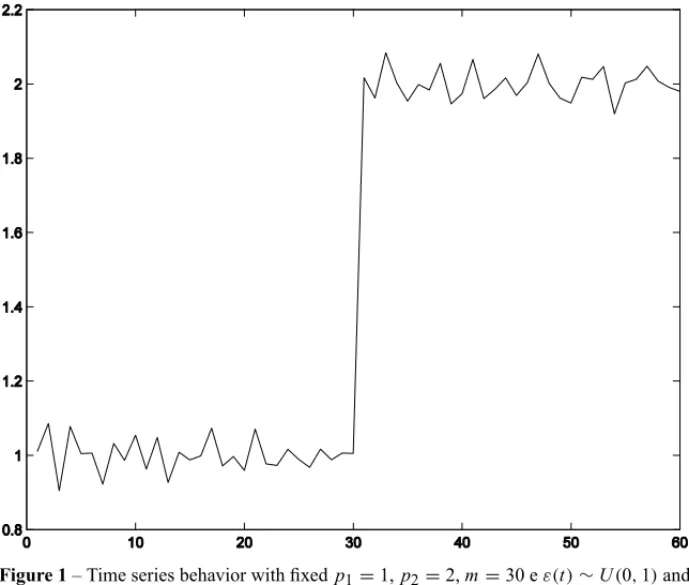
Assuming that p1is the first operation point, p2is the second operation point,ε(t)is the noise signal withπ(∙)distribution andmis the position of the change point, throughout the paper, it is considered the following time series:

f(t)= (

p1+0.1∗ε(t)−0.1∗ε(t−1), set≤m;

The Figure 1 show the time series behavior with fixedp1=1,p2=2,m=30 eε(t)∼U(0,1) and 60 samples of time series.

Figure 1– Time series behavior with fixedp1=1,p2=2,m=30 eε(t)∼U(0,1)and 60 samples of time series.

To establish notation, along this paper,U(0,1)denotes the uniform distribution in the interval [0,1],N(0,1)denotes the standard Normal distribution with zero mean and unit variance,t(5) denotes the Students-tdistribution with 5 degrees of freedom,gamma(a,b)denotes the Gamma distribution with scale parameteraand shape parameterbandŴ(a)denotes the gamma function evaluated ina. All the time series,e.g.,y(t), denotes a discrete-time sequence.

2 TIME SERIES TRANSFORMATION BY FUZZY SETS

One of the main applications of the fuzzy sets theory (Zadeh, 1965) is for clustering detection, in which the problem of grouping the data intokseparate categories is solved by defining different pertinences to each element belonging to category.

Thus, in this section, the first step of the proposed formulation to the change point detection problem is detailed, namely the fuzzy clustering of the initial time series.

Definition.Let y(t)be a time series, and consider a positive integer K . The set

C =

that solves the minimization problem

min k

X

i=1 X

μi(t)∈Ci

kμi(t)−Cik2 (2)

is called thefuzzy cluster centersset for the time series y(t). Thefuzzy membership degreeor fuzzy membership function value of y(t)∈ Ci (which means y(t)belongs to the cluster Ci) is given by

μi(t),1−(y(t)−Ci)2 k

X

j=1

(y(t)−Cj)2 (3)

Given the setC of cluster centers, it is an easy task to measure the distance between each point in the time seriesy(t)and each centerCi. The problem of finding the centers can be solved, for instance, viak-means (Kaufman & Rousseeuw, 1990),C-means (Bezdek, 1981), and Kohonen network (Kohonen, 2001). In this paper, the Kohonen network technique is used.

The proposed fuzzy clustering to transform a given time series into a new one is described below:

1. Input the time seriesy(t);

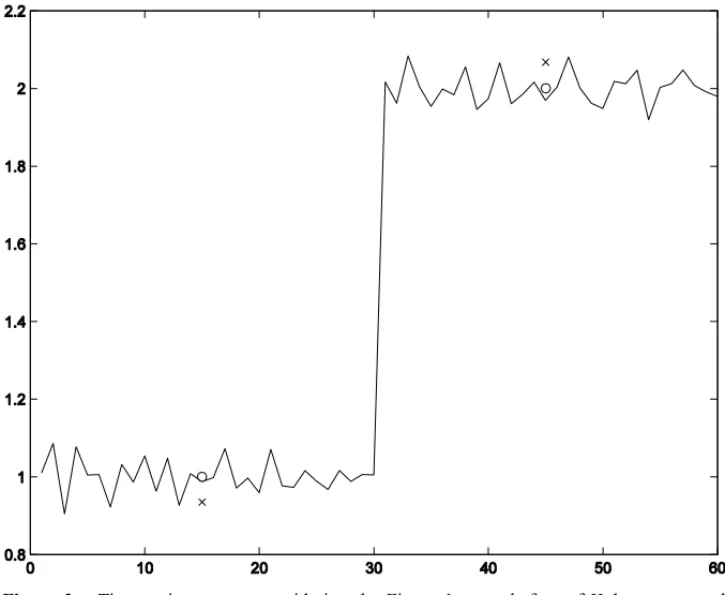
2. Find the set ofkcentersC= {Ci|min{y(t)} ≤Ci ≤max{y(t)},i =1,2}, that minimizes the Euclidean distance given in (2) and that is illustrated in Figure 2, considering, for example, the time series (1). For the proposal of this paper, it is consideredk=2 centers.

3. Compute the fuzzy membership degree given in (3), for each sample of the time series, y(t), with respect to each centerCi (as illustrated in Figure 3 considering, for example, the time series (1)).

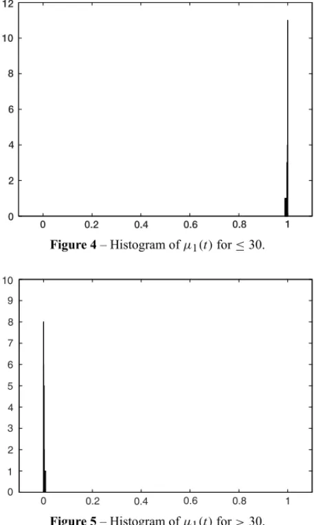
Since the idea is to find just one change point, only two centers are found. The functionμ1(t) defines a new time series, in which the change point is detected.

From Figure 3, it is noticeable that the fuzzy membership degree is concentrated around 1 (one) for the first 30 values observed before the change point (see also the histogram in Figure 4), and is concentrated around zero for the last 30 values observed after the change point (see also the histogram in Figure 5). Furthermore, the distribution ofμ1(t), defined according to (3), is confined into the interval[0,1], as shown below:

if y(t)−→C1 then μ1(t)−→1−;

if y(t)−→C2 then μ1(t)−→0+;

if C1−→C2 then μ1(t)−→1/2 ;

if y(t)−→ [C1,C2] then μ1(t)−→ [0,1].

Figure 2– Time series centers considering the Figure 1: ×– before of Kohonen network learning and◦– after of Kohonen network learning.

0 10 20 30 40 50 60

0 0.2 0.4 0.6 0.8 1

µ

1(t) µ₂(t)

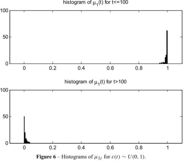
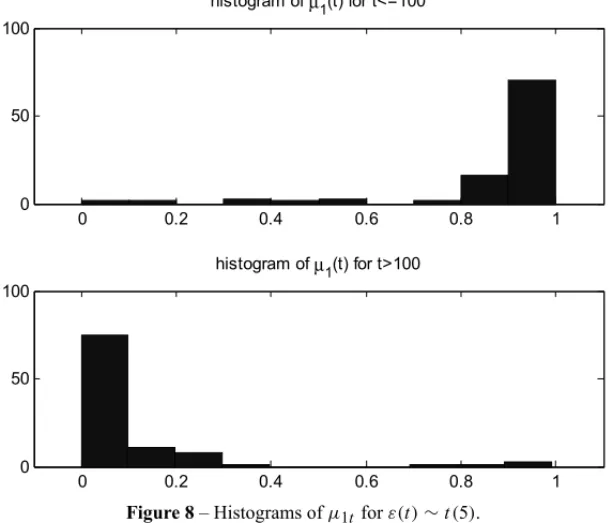
t > m it is assumed the beta(c,d)distribution. For example, in the case in which there is a change point in the time series, the parameter a is greater than the parameter in the Beta distribution ofμ1(t)ift ≤ m, and the parametercis smaller than the parameterd in the Beta distribution ofμ1(t)ift >m. Figures 6-8 presents an illustration of the distributions ofμ1(t)for the time series in (1) with sample sizen =200. It is assumed that the change point took place at the positionm=100. This empirical test has been performed starting from several time series, with different probability distributions for ε(t), say,U(0,1)in Figure 6, N(0,1)in Figure 7, andt(5)in Figure 8. In all these cases, the behavior of the transformed time series, obtained by applying the clustering technique, was well described by Beta distributions with similar shapes.

Figure 4– Histogram ofμ1(t)for≤30.

Figure 5– Histogram ofμ1(t)for>30.

0 0.2 0.4 0.6 0.8 1 0

50 100

histogram of µ₁(t) for t<=100

0 0.2 0.4 0.6 0.8 1

0 50 100

histogram of µ₁(t) for t>100

Figure 6– Histograms ofμ1t forε(t)∼U(0,1).

0 0.2 0.4 0.6 0.8 1

0 50 100

histogram of µ₁(t) for t<=100

0 0.2 0.4 0.6 0.8 1

0 50 100

histogram of µ₁(t) for t>100

0 0.2 0.4 0.6 0.8 1 0

50 100

histogram of µ

1(t) for t<=100

0 0.2 0.4 0.6 0.8 1

0 50 100

histogram of µ

1(t) for t>100

Figure 8– Histograms ofμ1t forε(t)∼t(5).

3 METROPOLIS-HASTINGS FORMULATION

The goal of the Metropolis-Hastings algorithm (Gamerman, 1997) is to construct a Markov chain that has a specified equilibrium distributionπ that in the paper is the posterior distribution of all parameters in the change point model.

Define a Markov chain as follows. IfXi−1=xi−1, then generate a candidate valuex∗=yfrom

a reference distribution with density fX∗_|X(y) = q(x_i−1,x∗). The candidate value x∗ is then

accepted or rejected as a sample ofπ. The acceptance probability is

α(x,y)=min

1, π(x

∗₎

π(xi−1)

q(x∗_,x i−1)

q(xi−1,x∗)

(4)

which defines the transition kernel of the chain. If the candidate is accepted, then set Xi =x∗, otherwise, set Xi = xi−1. It is possible to show that under general conditions the sequence

X0,X1,X2, . . .is a Markov chain with equilibrium distributionπ.

In practical terms, the Metropolis-Hastings algorithm can be specified by the following steps:

1. Choose a starting valuex0, the number of iterations,R, and set the iteration counterr =1;

2. Generate a candidate valuey∼q(xi,∙);

4. Compute the new value for the current state:

xt+1= (

y, if α(x,y) >u

xt, otherwise

5. Ifr<R, return to step 2. Otherwise stop.

As discussed in the previous section, the clustering technique generates a transformed time series with the following distribution

y(t)∼beta(a,b) , for t =1, . . . ,m y(t)∼beta(c,d) , for t =m+1, . . . ,n

where a,b,c,d and the change point m are the parameters to be estimated. To complete the model specification,prior distributionsare elicited for the parameters. As usually done when-ever there is no prior information available, in this paper the following non-informative prior distributions are assumed:

a ∼gamma(0.1,0.1)

b∼gamma(0.1,0.1)

c∼gamma(0.1,0.1)

d ∼gamma(0.1,0.1)

m∼U[1, . . . ,n], withp(m)=1/n.

These non-informative gamma prior distributions, with parameters 0.1, have been chosen with the purpose of spreading the whole parametric space.

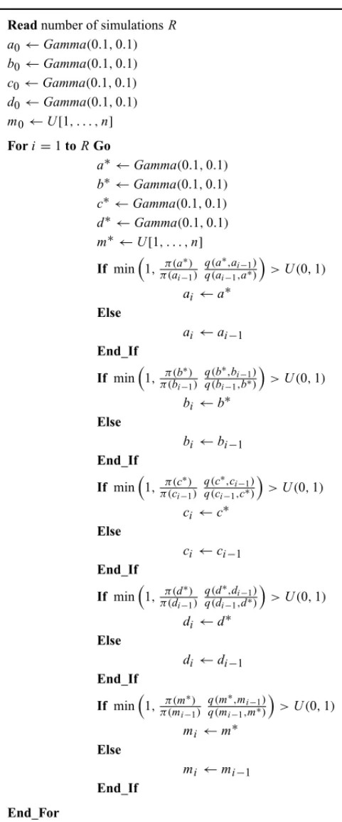
Since the posteriors do not have a close form, the Metropolis-Hastings algorithm is used to sample from them. Its formulation is given by the pseudo-code in the Table 1, and the reference distributions

π(a∗) π(ai−1)

q(a∗,ai−1)

q(ai−1,a∗)

, π(b

∗₎

π(bi−1)

q(b∗,bi−1)

q(bi−1,b∗)

, π(c

∗₎

π(ci−1)

q(c∗,ci−1)

q(ci−1,c∗)

,

π(d∗₎

π(di−1)

q(d∗_,d i−1)

q(di−1,d∗)

and π(m

∗₎

π(mi−1)

q(m∗_,m)

q(mi−1,m∗)

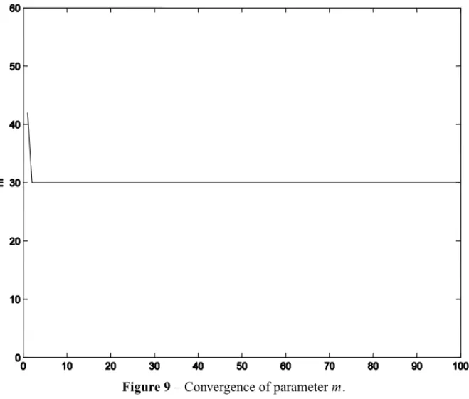
are presented in the Appendix A. The change pointm is obtained as the mode of its posterior distribution. It is approximated by the maximum value in the histogram for the R simulations of the pseudo-code in Table 1, with the exception of the border points of the distribution. The Figure 9 illustrates the convergence of parameterm for p1 =1,p2 =2, ε(t)∼U(0,1), R = 100 andm=30.

Table 1– Pseudo-code of the Metropolis-Hastings algorithm.

Readnumber of simulationsR a₀←Gamma(0.1,0.1)

b₀←Gamma(0.1,0.1)

c0←Gamma(0.1,0.1)

d0←Gamma(0.1,0.1)

m0←U[1, . . . ,n]

Fori=1toRGo

a∗←Gamma(0.1,0.1)

b∗←Gamma(0.1,0.1)

c∗←Gamma(0.1,0.1)

d∗←Gamma(0.1,0.1)

m∗←U[1, . . . ,n]

If min1,_π(π(_aa∗)

i−1)

q(a∗_,a i−1)

q(ai−1,a∗)

>U(0,1)

ai←a∗ Else

ai←ai−1

End If

If min1,_π(π(_bb∗)

i−1)

q(b∗_,b i−1)

q(bi−1,b∗)

>U(0,1)

bi←b∗ Else

bi←bi−1

End If

If min

1,_π(π(_cc∗)

i−1)

q(c∗_,c i−1)

q(ci−1,c∗)

>U(0,1)

ci←c∗ Else

ci←ci−1

End If

If min1,_π(π(_dd∗)

i−1)

q(d∗,di−1)

q(di−1,d∗)

>U(0,1)

d_i←d∗ Else

di←di−1

End If

If min1,_π(π(_mm∗)

i−1)

q(m∗_,m i−1)

q(mi−1,m∗)

>U(0,1)

mi ←m∗ Else

mi ←mi−1

End If

Figure 9– Convergence of parameterm.

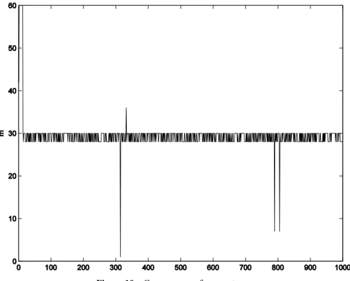
100% of correctness in detecting the change point in almost all situations. However, in the case when the time series changes from point p1=1 to point p2=1.1, the proposed approach has detected points in the neighborhood ofm=30, including it. In Table 2, the sign ‘XX’ indicates that the percentage of correctness was not conclusive. This fact is illustrated in the Figure 10, where a test was performed assumingp1=1,p2=1.1,ε(t)∼U(0,1),R=1000 andm=30. This behavior is due to the fact that both the noise and the signal change have the same amplitude.

Table 2– Results of change point detection.

p1 p2 m Noise size

% of correct % of correct % of correct detection detection detection

ε(t)∼U(0,1) ε(t)∼N(0,1) ε(t)∼t(5)

1 2 30 0.1 100 100 100

1 1.9 30 0.1 100 100 100

1 1.8 30 0.1 100 100 100

1 1.7 30 0.1 100 100 100

1 1.6 30 0.1 100 100 100

1 1.5 30 0.1 100 100 100

1 1.4 30 0.1 100 100 100

1 1.3 30 0.1 100 100 100

1 1.2 30 0.1 100 100 100

1 1.1 30 0.1 XX XX XX

Figure 10– Convergence of parameterm.

4 A CASE STUDY

The energy crisis faced by Brazil in early 2001 triggered a process of energy rationing in the country. This phenomenon was responsible for modifying habits and behaviors taken so far as standards when it came to consumption of electricity in Brazil. Since this fact has been occurred more useful studies to predict the electricity sector make necessary. In this case study the proposed methodology is used to assess the change in the trend at a particular time series that characterizes the energy consumption only in the Southeast Brazil (industry trade) in the period January 1976 to December 2000 (five months before the blackout in 2001), as presented in Figure 11, available at (IPEA).

Figure 11– Time series that characterizes the energy consumption only in the Southeast Brazil (industry trade) in the period January 1976 to December 2000.

Figure 12– Time series trend.

5 CONCLUSIONS

In this paper a novel fuzzy/Bayesian methodology for change point detection in time series was proposed. The methodology is based on a two step formulation. Firstly, a fuzzy clustering generates a transformed time series with Beta distribution to be used in the second step. In the second step, a Bayesian modeling is used for change point detection in the transformed time series. The Metropolis-Hastings algorithm is used to sample form the posteriors and the position of the change point is thus obtained taking the posterior mode as it estimation.

ACKNOWLEDGEMENTS

This work has been supported by Brazilian agencies FAPEMIG and CNPq.

REFERENCES

[1] BARRY D & HARTIGAN JA. 1993. A Bayesian Analysis for Change Point Problems, 88(421): 309–319.

[2] BECKAGEB, JOSEPHL, BELISLEP, WOLFSONDB & PLATTWJ. 2007. Bayesian change-point analyses in ecology.New Phytologist,174: 456–467.

[3] BEZDEKJC. 1981.Pattern recognition with fuzzy objective function algorithms. Plenum Press. [4] GAMERMAN D. 1997.Markov chain Monte Carlo: stochastic simulation for Bayesian inference.

Chapman & Hall.

[5] HADJILIADISO & MOUSTAKIDESV. 2006. Optimal and Asymptotically Optimal CUSUM Rules for Change Point Detection in the Brownian Motion Model with Multiple Alternatives.Theory of Probability and its Applications,50(1): 75–85.

[6] HARTIGANJA. 1990. Partition Models,19(8): 2745–2756.

[7] HINKEYDV. 1971. Inference About the Change Point from Cumulative Sum Test,26: 279–284. [8] HODRICKR & PRESCOTT EC. 1997. Postwar U.S. Business Cycles: An Empirical Investigation.

Journal of Money, Credit, and Banking,29: 1–16.

[9] IPEA – INSTITUTO DEPESQUISASECONOMICAˆ APLICADA. (n.d.). Retrieved may 10, 2008, from http://www.ipeadata.gov.br.

[10] KAUFMANL & ROUSSEEUWPJ. 1990.Finding groups in data: An introduction to cluster analysis. John Wiley & Sons.

[11] KOHONENT. 2001.Self-organizing maps. Springer.

[12] KULLBACKS & LEIBLERRA. 1951. On Information and Sufficiency.Annals of Mathematical Sta-tistics,22(1): 79–86.

[13] LEES, NISHIYAMAY & YOSHIDAN. 2006. Test for Parameter Change in Diffusion Processes by Cusum Statistics Based on One-step Estimators.Annals of the Institute of Statistical Mathematics, 58(2): 211–222.

[15] LOSCHI RH & CRUZ FRB. 2005. Bayesian Identification of Multiple Change Points in Poisson Data.Advances in Complex Systems,8: 465–482.

[16] LOSCHIRH & CRUZFRB. 2005. Extension to the product partition model: computing the probabi-lity of a change.Computational Statistics and Data Analysis,48(2): 255–268.

[17] LOSCHIRH, GONC¸ALVESFB & CRUZFBR. 2005. Avaliac¸˜ao de uma medida de evidˆencia de um ponto de mudanc¸a e sua utilizac¸˜ao na identificac¸˜ao de mudanc¸as na taxa de criminalidade em Belo Horizonte.Pesquisa Operacional,25(3): 459–463.

[18] OH KJ, ROH TH & MOONMS. 2005. Developing time-based clustering neural networks to use change-point detection: Application to financial time series.Asia-Pacific Journal of Operational Re-search,22(1): 51–70.

[19] ZADEHLA. 1965. Fuzzy Sets.Information and Control,8(3): 338–353.

A Appendix

In this appendix is presented the acceptance probability for theposteriordistribution of the pa-rametersa,b,c,d andmdescribed in the Metropolis-Hastings algorithm. The reference distri-butions used in the work are thepriordistributionsgamma(0.1,0.1).

The reference distribution in Metropolis-Hastings is computed by likelihood function:

f(y|a,b,c,d,m)∼ m

Y

i=1

Ŵ(a+b) Ŵ(a)+Ŵ(b)y

a−1 i (1−yi)

b−1 m

Y

i=m+1

Ŵ(c+d) Ŵ(c)+Ŵ(d)y

c−1 i (1−yi)

d−1

1. For the parametera:

π(a∗) π(ai−1)

q(a∗,ai−1) q(ai−1,a∗)

= π(a

∗₎

π(ai−1)

f(y|a∗,bi−1,ci−1,di−1,mi−1)π(a∗)π(bi−1)π(ci−1)π(di−1)π(mi−1) f(y|ai−1_,bi−1_,ci−1_,di−1_,mi−1_)π(ai−1_)π(bi−1_)π(ci−1_)π(di−1_)π(mi−1₎

= h

Ŵ(a∗_+bi−1₎ Ŵ(a∗_)Ŵ(bi−1₎

imi−1h

Ŵ(ci−1_+di−1₎ Ŵ(ci−1_)Ŵ(d)

in−mi−1 Qmi−1

j=1 h

ya_j∗−1(1−yj)b i−1₋₁i h

Ŵ(ai−1_+bi−1₎ Ŵ(ai−1_)Ŵ(bi−1₎

imi−1h

Ŵ(ci−1_+di−1₎ Ŵ(ci−1_)Ŵ(di−1₎

in−mi−1 Qmi−1

j=1 h

ya_ji−1−1(1−yj)bi−1−1

i

× Qn

j=mi−1₊₁ h

yc_ji−1−1(1−yj)d i−1₋₁i Qn

j=mi−1₊₁ h

yc_ji−1−1(1−yj)di−1−1

i h

0.10.1[Ŵ(0.1)]−1a∗0.1−1e−0.1a∗i2

h

0.10.1_[Ŵ(0.1)]−1_ai−10.1−1

e−0.1ai−1i2

= h

Ŵ(a∗_+bi−1₎ Ŵ(a∗₎

imi−1 Qmi−1

j=1 ya

∗₋₁

j

h

ai−1

a∗

i0.9

e−0.1(a∗−ai−1) 2

h

Ŵ(ai−1_+bi−1₎ Ŵ(ai−1₎

imi−1 Qmi−1

j=1 y ai−1₋₁

2. For the parameterb:

π(b∗) π(bi−1)

q(b∗,bi−1)

q(bi−1,b∗)

= π(b

∗₎

π(bi−1)

f(y|ai,b∗,ci−1,di−1,mi−1)π(ai)π(b∗)π(ci−1)π(di−1)π(mi−1) f(y|ai_,bi−1_,ci−1_,di−1_,mi−1_)π(ai_)π(bi−1_)π(ci−1_)π(di−1_)π(mi−1₎

= h

Ŵ(ai_+b∗₎

Ŵ(ai_)Ŵ(b∗₎

imi−1h

Ŵ(ci−1_+di−1₎ Ŵ(ci−1_)Ŵ(d)

in−mi−1 Qmi−1

j=1 h

ya_ji−1(1−yj)b

∗₋₁i

h_Ŵ(ai_+bi−1₎ Ŵ(ai_)Ŵ(bi−1₎

imi−1h _Ŵ(ci−1_+di−1₎ Ŵ(ci−1_)Ŵ(di−1₎

in−mi−1 Qmi−1

j=1 h

ya_ji−1(1−yj)bi−1−1

i

× Qn

j=mi−1₊₁ h

yc_ji−1−1(1−yj)d i−1₋₁i Qn

j=mi−1₊₁ h

yc_ji−1−1(1−yj)di−1−1

i h

0.10.1_[Ŵ(0.1)]−1_b∗0.1−1_e−0.1b∗i2

h

0.10.1_[Ŵ(0.1)]−1_bi−10.1−1

e−0.1bi−1i2

= h

Ŵ(ai+b∗) Ŵ(b∗₎

imi−1 Qmi−1

j=1(1−yj)b

∗₋₁h

bi−1

b∗

i0.9

e−0.1(b∗−bi−1) 2

h

Ŵ(ai−1_+bi−1₎ Ŵ(bi−1₎

imi−1 Qmi−1

j=1(1−yj)bi−1−1 3. For the parameterc:

π(c∗₎

π(ci−1)

q(c∗_,c i−1)

q(ci−1,c∗)

= π(c

∗₎

π(ci−1)

f(y|ai,bi,c∗,di−1,mi−1)π(ai)π(bi)π(c∗)π(di−1)π(mi−1) f(y|ai_,bi_,ci−1_,di−1_,mi−1_)π(ai_)π(bi_)π(ci−1_)π(di−1_)π(mi−1₎

= h

Ŵ(ai_+bi₎

Ŵ(ai_)Ŵ(bi₎

imi−1h

Ŵ(c∗_+di−1₎ Ŵ(c∗_)Ŵ(di−1₎

in−mi−1 Qmi−1

j=1 h

ya_ji−1(1−yj)b i₋₁i h _Ŵ(ai_+bi₎

Ŵ(ai_)Ŵ(bi₎

imi−1h_Ŵ(ci−1_+di−1₎ Ŵ(ci−1_)Ŵ(di−1₎

in−mi−1 Qmi−1

j=1 h

ya_ji−1(1−yj)bi−1

i

× Qn

j=mi−1₊₁ h

yc_j∗−1(1−yj)d i−1₋₁i Qn

j=mi−1₊₁ h

yc_ji−1−1(1−yj)di−1−1

i h

0.10.1[Ŵ(0.1)]−1c∗0.1−1e−0.1c∗i 2

h

0.10.1_[Ŵ(0.1)]−1_ci−10.1−1

e−0.1ci−1i2

= h

Ŵ(c∗_+di−1₎ Ŵ(c∗₎

in−mi−1 Qn

j=mi−1₋₁yc

∗₋₁

j

_h

ci−1 c∗

i0.9

e−0.1(c∗−ci−1) 2

h_Ŵ(ci−1_+di−1₎ Ŵ(di−1₎

in−mi−1 Qn

j=mi−1₊₁y

ci−1₋₁

j

4. For the parameterd:

π(d∗) π(di−1)

q(d∗,di−1)

= π(d ∗₎

π(di−1)

f(y|ai,bi,ci,d∗,mi−1)π(ai)π(bi)π(ci)π(d∗)π(mi−1) f(y|ai_,bi_,ci_,di−1_,mi−1_)π(ai_)π(bi_)π(ci_)π(di−1_)π(mi−1₎

= h

Ŵ(ai_+bi₎

Ŵ(ai_)Ŵ(bi₎

imi−1h

Ŵ(ci_+d∗₎

Ŵ(ci_)Ŵ(d∗₎

in−mi−1 Qmi−1

j=1 h

ya_ji−1(1−yj)b i₋₁i h

Ŵ(ai_+bi₎

Ŵ(ai_)Ŵ(bi₎

imi−1h

Ŵ(ci_+di−1₎ Ŵ(ci_)Ŵ(di−1₎

in−mi−1 Qmi−1

j=1 h

ya_ji−1(1−yj)bi−1

i

× Qn

j=mi−1₊₁ h

yc_ji−1(1−yj)d

∗₋₁i

Qn

j=mi−1₊₁ h

yc_ji−1(1−yj)di−1−1

i h

0.10.1[Ŵ(0.1)]−1d∗0.1−1e−0.1d∗i2

h

0.10.1_[Ŵ(0.1)]−1_di−10.1−1

e−0.1di−1i2

= h

Ŵ(c∗_+di−1₎ Ŵ(c∗₎

in−mi−1 Qn

j=mi−1₋₁ h

(1−yj)d

∗₋₁ih

di−1

d∗

i0.9

e−0.1(d∗−di−1) 2

h

Ŵ(ci−1_+di−1₎ Ŵ(di−1₎

in−mi−1 Qn

j=mi−1₊₁ h

(1−yj)di−1−1

i

5. For the parameterm:

π(m∗) π(mi−1)

q(m∗,m) q(mi−1,m∗)

= π(m

∗₎

π(mi−1)

f(y|ai,bi,ci,di,m∗)π(ai)π(bi)π(ci)π(di)π(m∗) f(y|ai_,bi_,ci_,di_,mi−1_)π(ai_)π(bi_)π(ci_)π(di_)π(mi−1₎

Sendoπ(m(∙)_{)∼U(0,1), ent˜ao:}

π(m∗)

π(m_i−1)

q(m∗,m)

q(m_i−1,m∗₎

= f(y|a

i_,bi_,ci_,di_,m∗₎

f(y|ai_,bi_,ci_,di_,mi−1₎

= h

Ŵ(ai_+bi₎

Ŵ(ai_)Ŵ(bi₎

im∗h

Ŵ(ci_+di₎

Ŵ(ci_)Ŵ(di₎

in−m∗ Qm∗

j=1 h

ya_ji−1(1−yj)b i₋₁i

Qn

j=m∗₊₁

h

yc_ji−1(1−yj)d i₋₁i h _Ŵ(ai_+bi₎

Ŵ(ai_)Ŵ(bi₎

imi−1h _Ŵ(ci_+di₎

Ŵ(ci_)Ŵ(di₎

in−mi−1 Qmi−1

j=1 h

ya_ji−1(1−yj)bi−1

i Qn

j=mi−1₊₁ h

yc_ji−1(1−yj)di−1