❊♥s❛✐♦s ❊❝♦♥ô♠✐❝♦s
❊s❝♦❧❛ ❞❡
Pós✲●r❛❞✉❛çã♦
❡♠ ❊❝♦♥♦♠✐❛
❞❛ ❋✉♥❞❛çã♦
●❡t✉❧✐♦ ❱❛r❣❛s
◆
◦
✹✽✽
■❙❙◆ ✵✶✵✹✲✽✾✶✵
❇♦✉♥❞s ❢♦r t❤❡ ♣r♦❜❛❜✐❧✐t② ❞✐str✐❜✉t✐♦♥ ❢✉♥❝✲
t✐♦♥ ♦❢ t❤❡ ❧✐♥❡❛r ❆❈❉ ♣r♦❝❡ss
▼❛r❝❡❧♦ ❋❡r♥❛♥❞❡s
❖s ❛rt✐❣♦s ♣✉❜❧✐❝❛❞♦s sã♦ ❞❡ ✐♥t❡✐r❛ r❡s♣♦♥s❛❜✐❧✐❞❛❞❡ ❞❡ s❡✉s ❛✉t♦r❡s✳ ❆s
♦♣✐♥✐õ❡s ♥❡❧❡s ❡♠✐t✐❞❛s ♥ã♦ ❡①♣r✐♠❡♠✱ ♥❡❝❡ss❛r✐❛♠❡♥t❡✱ ♦ ♣♦♥t♦ ❞❡ ✈✐st❛ ❞❛
❋✉♥❞❛çã♦ ●❡t✉❧✐♦ ❱❛r❣❛s✳
❊❙❈❖▲❆ ❉❊ PÓ❙✲●❘❆❉❯❆➬➹❖ ❊▼ ❊❈❖◆❖▼■❆
❉✐r❡t♦r ●❡r❛❧✿ ❘❡♥❛t♦ ❋r❛❣❡❧❧✐ ❈❛r❞♦s♦
❉✐r❡t♦r ❞❡ ❊♥s✐♥♦✿ ▲✉✐s ❍❡♥r✐q✉❡ ❇❡rt♦❧✐♥♦ ❇r❛✐❞♦
❉✐r❡t♦r ❞❡ P❡sq✉✐s❛✿ ❏♦ã♦ ❱✐❝t♦r ■ss❧❡r
❉✐r❡t♦r ❞❡ P✉❜❧✐❝❛çõ❡s ❈✐❡♥tí✜❝❛s✿ ❘✐❝❛r❞♦ ❞❡ ❖❧✐✈❡✐r❛ ❈❛✈❛❧❝❛♥t✐
❋❡r♥❛♥❞❡s✱ ▼❛r❝❡❧♦
❇♦✉♥❞s ❢♦r t❤❡ ♣r♦❜❛❜✐❧✐t② ❞✐str✐❜✉t✐♦♥ ❢✉♥❝t✐♦♥ ♦❢
t❤❡ ❧✐♥❡❛r ❆❈❉ ♣r♦❝❡ss✴ ▼❛r❝❡❧♦ ❋❡r♥❛♥❞❡s ✕ ❘✐♦ ❞❡ ❏❛♥❡✐r♦ ✿
❋●❱✱❊P●❊✱ ✷✵✶✵
✭❊♥s❛✐♦s ❊❝♦♥ô♠✐❝♦s❀ ✹✽✽✮
■♥❝❧✉✐ ❜✐❜❧✐♦❣r❛❢✐❛✳
Bounds for the probability distribution function
of the linear ACD process
Marcelo Fernandes
Graduate School of Economics, Funda¸c˜
ao Getulio Vargas
Praia de Botafogo, 190, 22253-900 Rio de Janeiro, Brazil
Tel: +55 21 2559 5827
Fax: +55 21 2553 8821
E-mail:
[email protected]
Abstract:
This paper derives both lower and upper bounds for the probability
distribution function of stationary ACD(p, q) processes. For the purpose of
illustration, I specialize the results to the main parent distributions in duration
analysis. Simulations show that the lower bound is much tighter than the upper
bound.
JEL Classification:
C22, C41.
Acknowledgements:
I am grateful to Bernardo de S´a Mota for excellent
re-search assistance and to the CNPQ for supporting this rere-search. The usual
1
Introduction
The statistical properties of the autoregressive conditional duration model of
first order are by now quite well known. Engle and Russell (1998) derive not
only the first two moments of the ACD(1,1) model, but also the conditions
un-der which it is stationary and
β
−
mixing. Carrasco and Chen (2002) extend the
latter results so as to consider the more general ACD(p, q) model. Bauwens and
Giot (2000) provide a recursive formula to compute the autocorrelation
func-tion of the ACD(1,1) process with exponential errors. Fernandes and Grammig
(2002) establish conditions for the existence of higher-order moments, strict
stationarity and
β
−
mixing property as well as moment recursion relations and
autocovariance function of a richer class of nonlinear ACD(1,1) processes that
encompasses most autoregressive conditional duration models in the literature.
This note aims at deriving nonasymptotic characterizations of the tail
be-havior of unconditional distribution function of the ACD(p, q) process. More
precisely, I derive both lower and upper bounds for the probability density
func-tion of the durafunc-tion process. These bounds are quite relevant to the analysis of
liquidity risk in that trade and volume durations are intimately related to
mar-ket activity and liquidity (see Gouri´eroux, Jasiak and Le Fol, 1999). Another
interesting application relates to actuarial models of credit risk contagion as in
Focardi (2001).
The remainder of this paper is organized as follows. Section 2 bounds the
probability density function of the ACD(p, q) process without assuming a
partic-ular distribution for the error term. Section 3 sharpens the result by considering
the usual specifications of the density of the error term. Section 4 investigate
the precision of these bounds through a simple simulation study.
2
Bounds
Let
x
t
=
τ
t
−
τ
t
−
1
denote the time spell between two events occurring at times
τ
t
and
τ
t
−
1. Engle and Russell (1998) propose to account for the serial dependence
where
ψ
t
≡
E
¡
x
t
|
Ω
t
−
1
¢
,
ǫ
t
is iid with unity mean, and Ω
t
−
1
is the set including
all information available at time
τ
t
−
1. The ACD(p, q) then assumes that
ψ
t
and
ǫ
t
are stochastically independent, and
ψ
t
=
ω
+
p
X
i
=1
α
i
x
t
−
i
+
q
X
j
=1
β
j
ψ
t
−
j
,
(1)
where
ω >
0,
α
≡
(α1, . . . , α
p
)
≥
0, and
β
≡
(β1, . . . , β
q
)
≥
0. This
param-eter restrictions ensure the nonnegativeness of the duration process, whereas
imposing
γ
≡
P
p
i
=1
α
i
+
P
q
j
=1
β
j
<
1 guarantees stationarity.
I take benefit from the close parallel between ACD and GARCH models in
order to establish both lower and upper bounds of the probability distribution
function. More precisely, I start with a trivial upper bound and then derive a
nontrivial lower bound using the techniques put forth by Pawlak and Schmid
(2001). Denoting by
F
ǫ
the probability distribution function of the error term,
it follows that
Pr(x
t
≤
z) =
E
£
Pr
¡
ψ
t
ǫ
t
< z
|
I
t
−
1
¢¤
=
E
"
F
ǫ
Ã
z
ω
+
P
p
i
=1
α
i
x
t
−
i
+
P
q
j
=1
β
j
ψ
t
−
j
!#
.
(2)
It is readily seen that
Pr(x
t
≤
z)
≤
F
ǫ
(z/ω)
(3)
given that durations are nonnegative as well as
α
and
β
.
As in Pawlak and Schmid (2001), the nontrivial lower bound for the
prob-ability distribution function of the duration process holds only for
z
∈
[0,
z],
¯
where ¯
z
varies according to the distribution of the error term. The reason is
that, to apply Jensen’s inequality to bound (2) from below, one must find the
conditions under which the function
H
(u, v) =
F
ǫ
Ã
z
ω
+
P
p
i
=1
α
i
u
i
+
P
q
j
=1
β
j
v
j
!
(4)
is convex for all
u
≡
(u1, . . . , u
p
)
≥
0 and
v
≡
(v1, . . . , v
q
)
≥
0. It is
straightfor-ward to show that the Hessian of (4) is convex if
2f
ǫ
(z/M) +
z
M
f
′
where
M
=
ω
+
P
p
i
=1
α
i
u
i
+
P
q
j
=1
β
j
v
j
, given that
∂
2
H
(u, v)
∂u
r
∂u
s
=
α
r
α
s
z
2
M
4
f
′
ǫ
(z/M
) + 2
α
r
α
s
z
M
3
f
ǫ
(z/M)
(6)
∂
2
H
(u, v)
∂u
r
∂v
s
=
α
r
β
s
z
2
M
4
f
ǫ
′
(z/M
) + 2
α
r
β
s
z
M
3
f
ǫ
(z/M)
(7)
∂
2
H
(u, v)
∂v
r
∂u
s
=
β
r
β
s
z
2
M
4
f
′
ǫ
(z/M) + 2
β
r
β
s
z
M
3
f
ǫ
(z/M
)
(8)
for
r
6
=
s. I am now ready to state the main result.
Theorem.
Let
x
t
∼
ACD(p, q)
satisfying the nonnegativeness and stationarity
conditions. Assuming that the density
f
ǫ
of the error term is differentiable then
yields that
F
ǫ
(x)
≤
Pr
µ
x
t
≤
ω
1
−
γ
x
≤
F
ǫ
µ
x
1
−
γ
,
(9)
where the lower bound holds only for
x
∈
£
0,
(1
−
γ)c
¤
with
c
≡
sup
τ >
0
n
2f
ǫ
(x) +
xf
ǫ
′
(x)
≥
0 for all 0
< x < τ
o
.
(10)
Proof.
It ensues from condition (5) that
sup
τ >
0
n
2f
ǫ
(z/M) +
z
M
f
′
ǫ
(z/M
)
≥
0 for all 0
< x < τ
o
=
M
sup
τ >
0
{
2f
ǫ
(x) +
xf
ǫ
′
(x)
≥
0 for all 0
< x < τ
}
=
M c.
(11)
The Hessian of (4) is therefore convex if
z
≤
c
ω
+
p
X
i
=1
α
i
u
i
+
q
X
j
=1
β
j
v
j
.
(12)
This is true for any
α
i
, ui, β
j
, v
j
≥
0 if
z
≤
cω. The result then follows by
applying the Jensen’s inequality to (2) with
z
=
1
−
ω
γ
x.
¥
As is apparent, the applicability of the lower bound depends essentially on
the constant
c, and hence it is interesting to evaluate (10) for the usual
dis-tributions in the ACD literature. I therefore consider in the next section five
particular cases, namely exponential, Weibull, Burr, generalized gamma, and
uniform. In all instances I normalize the distribution so as to impose unity
3
Examples
The ACD modeling aims to match two stylized features in financial
dura-tion data, namely serial correladura-tion and overdispersion.
Engle and Russell
(1998) show indeed that the simple ACD model with exponential errors produce
overdispersion. Further, quasi maximum likelihood methods provide consistent
estimates for ACD process only if based on the exponential distribution (see
Drost and Werker, 2001). It seems therefore natural to start with the
exponen-tial assumption for the error term, which yields
f
E
(x) =
e
−
x
and
f
E
′
(x) =
−
e
−
x
.
By (5), this implies that
c
= 2.
Engle and Russell (1998) argue that the nature of financial durations are
more in line with a decreasing baseline hazard rate function. The exponential
assumption implies however that the baseline hazard rate function is flat. A
natural candidate then is the Weibull distribution with parameter
θ, which
gives rise to either monotonically decreasing (0
< θ <
1) or increasing (θ >
1)
baseline hazard rate functions. The density function of the Weibull distribution
and its first derivative are
f
W
(x) =
θ
Γ(1 + 1/θ)
x
θ
−
1
exp
·
−
x
θ
Γ(1 + 1/θ)
¸
(13)
f
′
W
(x) =
−
f
W
(x)
·
1
−
θ
x
+
θ
Γ(1 + 1/θ)
x
θ
−
1
¸
,
(14)
respectively. Condition (5) then becomes
f
W
(x)
·
2
−
1 +
θ
−
Γ(1 + 1/θ)
θ
x
θ
¸
≥
0,
(15)
which implies that
c
=
h
Γ(2 + 1/θ)
i
1
/θ
. As a sanity check, observe that in the
exponential case
θ
= 1, recovering
c
= Γ(3) = 2. If one assumes that 0
< θ <
1
as in Engle and Russell (1998), then the sup condition in (10) becomes less
stringent than in the exponential context, viz.
c >
2.
Grammig and Maurer (2000) advocate the use of the Burr distribution in
order to accommodate more flexible hazard rate functions. Indeed the Burr
density
f
B
(x) =
θ ξ
θ
B
x
θ
−
1
¡
1 +
κ ξ
θ
B
x
θ
where
θ > κ >
0 and
ξ
B
≡
Γ
¡
1 + 1/θ
¢
Γ
¡
1/κ
−
1/θ
¢
κ
1+1
/θ
Γ
¡
1 + 1/κ
¢
,
(17)
entails a nonmonotonic baseline hazard rate function if
θ >
1. It is easy to show
that
f
′
B
(x) =
f
B
(x)
·
θ
−
1
x
−
µ
1 +
1
κ
κ θ ξ
θ
B
x
θ
−
1
1 +
κ ξ
θ
B
x
θ
¸
,
(18)
and hence
c
=
µ
θ
+ 1
θ
−
κ
1
/θ
ξ
−
1
B
=
µ
θ
+ 1
θ
−
κ
1
/θ
κ
1+1
/θ
Γ(1 + 1/κ)
Γ(1 + 1/θ) Γ(1/κ
−
1/θ)
.
(19)
Special cases of the Burr family of distributions are the Weibull (κ
→
0), the
exponential (κ
→
0, θ
= 1), and the log-logistic (θ > κ
= 1) distributions.
As an alternative to the Burr model, Lunde (1999) puts forward the
gener-alized gamma ACD process, where
ǫ
t
is iid with density
f
G
(x) =
ξ
θκ
G
θx
θκ
−
1
Γ(κ)
exp
¡
−
ξ
G
θ
x
θ
¢
(20)
where
ξ
G
≡
Γ(κ
+ 1/θ)/Γ(κ). The generalized gamma distribution nests the
standard gamma (θ
= 1), log-normal (κ
→ ∞
), Weibull (κ
= 1), exponential
(θ
=
κ
= 1), and half-normal (κ
= 1/2, θ
= 2) distributions.
Although the baseline hazard rate has no closed-form solution, it is possible
to derive its shape properties according to the parameter values (Glaser, 1980).
If
θκ <
1, the hazard rate is decreasing for
θ
≤
1, and U-shaped for
θ >
1.
Conversely, if
θκ >
1, the hazard rate is increasing for
θ
≥
1, and inverted
U-shaped for
θ <
1. Lastly, if
θκ
= 1, the hazard rate is decreasing for
θ <
1,
constant for
θ
= 1 (exponential case), and increasing for
θ >
1. The derivative
of the density is
f
′
G
(x) =
f
G
(x)
·
κθ
−
1
x
−
θ ξ
θ
G
x
θ
−
1
¸
,
(21)
yielding
c
= (κ
+ 1/θ)
1
/θ
Γ(κ)
Γ(κ
+ 1/θ)
.
(22)
It is easy to show that the lower bound is valid for
c
=
√
π
and
c
= 1 + 1/κ
in the particular cases of the half-normal and standard gamma distributions,
Finally, albeit the ACD process with
ǫ
t
∼
U
(0,
2) does not have much appeal
in practice, it entails a very interesting result. Indeed, it turns out that (5) holds
for every value of
x, and so the lower bound is always valid. Figure 1 summarizes
these results by displaying the constant
c
as a function of the distributional
parameters. There are no plots for the exponential, half-normal and uniform
distributions in view that
c
does not vary for them.
4
Sharpness of the bounds
To investigate how tight these bounds are, I perform a simple simulation study
using an ACD(2,2) process with exponential errors. I set
α
= (0.10,
0.05) and
β
= (0.45,
0.25) and normalize the unconditional expected duration to one by
imposing
ω
= 1
−
γ. Next, I initialize (1) with
ψ0
= 1 and simulate 10,000
realizations of the process and then estimate the unconditional cumulative
dis-tribution of the duration process using the empirical disdis-tribution of the last
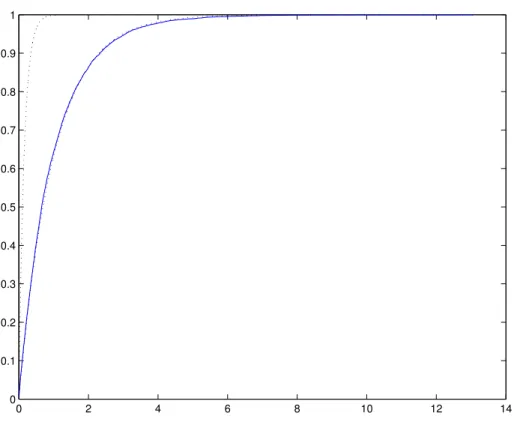
8,000 observations of the sample. Figure 2 illustrates the fact that, despite
the slackness of the trivial upper limit, the nontrivial lower bound is extremely
sharp and informative. Further simulations show that this result is quite robust
to the specification of the linear ACD process. The simulations also indicate
that by substituting maximum likelihood estimates for the true values of the
parameters, the 95% confidence interval of the lower bound provides a tight
confidence band to the true probability distribution function of the process.
References
Bauwens, L., Giot, P., 2000, The logarithmic ACD model: An application to
the bid-ask quote process of three NYSE stocks, Annales d’Economie et de
Statistique 60, 117–150.
Carrasco, M., Chen, X., 2002, Mixing and moment properties of various GARCH
and stochastic volatility models, Econometric Theory 18, 17–39.
Engle, R. F., Russell, J. R., 1998, Autoregressive conditional duration: A new
model for irregularly-spaced transaction data, Econometrica 66, 1127–1162.
Fernandes, M., Grammig, J., 2002, A family of autoregressive conditional
dura-tion models, Ensaios Econˆ
omicos 404, Funda¸c˜
ao Getulio Vargas.
Focardi, S. M., 2001, An actuarial model of credit risk contagion, Discussion
Paper 03, Intertek Group.
Glaser, R. E., 1980, Bathtub and related failure rate characterizations, Journal
of the American Statistical Association 75, 667–672.
Gouri´eroux, C., Jasiak, J., Le Fol, G., 1999, Intra-day market activity, Journal
of Financial Markets 2, 193–226.
Grammig, J., Maurer, K.-O., 2000, Non-monotonic hazard functions and the
autoregressive conditional duration model, Econometrics Journal 3, 16–38.
Lunde, A., 1999, A generalized gamma autoregressive conditional duration
model, University of Aarhus.
1
2
3
4
5
1
1.5
2
θ
c
0.2
0.4
0.6
0.8
1
0
1
2
3
x 10
5
θ
c
0
2
4
6
8
10
0.38
0.39
0.4
0.41
0.42
k
c
0
2
4
6
8
10
0
5
10
15
k
c
0
5
0
5
1
2
3
θ
k
c
0
5
5
10
0
1
2
θ
k
c
Figure 1: The constant
c
as a function of the distributional parameters
coordinates
distribution
(1,1)
Weibull (
θ
≥
1)
(1,2)
Weibull (
θ
≤
1)
(2,1)
log-logistic
(2,2)
gamma
(3,1)
generalized gamma
0
2
4
6
8
10
12
14
0
0.1
0.2
0.3
0.4
0.5
0.6
0.7
0.8
0.9
1
Figure 2: Bounds for the linear ACD probability distribution function
✘✙✟✖☞✍✫✵✴✶✝✠✷✹✸✻✺✹✼✹✽✾❀✿★✼✹✸✻❁★✷✹❁★❂☛✼✹❃❅❄❇❆✙❈☛✷✹❁❉✕✓✾★✸✻✾❉✴❊☞✍❋☛✸✻●❍✽■❂☛✼❑❏✁▲✄▲✄❏✥✴✶✂✁✂◆▼☛❖✹P✁❃✬☎
✁✄✄☎ ☞◗✘✙✆✔✪✜❘❙✑☛✕❚✭✰✆✰❯✵✟★✘✁✕☛❱✦✭✰✘✙✆✔✿★✎✚✫❲✟❳✿☛✆✔✘❨✪✜✘✁☞✵❩❬✎✒✫◆❘✩✑✓✎✒✌✏❭❪✝✠❘❙✫❫✕✙✎✒✭✰✫✬✟❴✛❇☞✵✕☛☞❵✑❛✆✩❘✩✘✙✡✙✟★✑❴✴✞✿★✸✻✷✹❁★✺✹●❜❃✬✺✹✾
❝
☎✁❭✩☎✁✿★✼✹✸✻✸✻✼✹●❍✸✻✷❞❄✜✭✰✼❞❡✳✼✹✸❛✫✬✷✹❁✖❢❣✾★❈✖❤◆❄✜✝✠✷✹✸✐✺✹✼✹✽✾❀✌✏✼✹✸✐●❞✴❊☞✍❋☛✸✻●❍✽■❂☛✼❑❏✄▲✁▲✄❏✥✴✶✂✄❥❦▼✁❖✹P☛❃■☎
✁✄❧✄☎ ✕ ❝ ✟♠✝✠✎✚✑✓✑❛✎✚✌✣❭ ✫❲✎✚✌✣♥✄♦♣❘✩✑✓✎✒✌✏❭q✕ ❝ ✟r✌✏✪✜✟★✘ ✘✙✟★✡✙✟★✑❛✑✓✎✚✆✔✌ ✎✚✌✣✛✔✎✒✡✁☞✵✕✓✆✩✘♠✕✙✆ ✡✙✆✔✌✏✑★✕✙✘✙❘✩✡✁✕ ✡✙✆✔✎✚✌✣✡✙✎✚✛✜✟★✌✜✕❴☞✥✌✏✛s✫✬✟✖☞✍✛✜✎✚✌✣❭❨✎✒✌✏✛✜✎✚✡✓✟☛✑✠✆✔✿t✟★✡✙✆✔✌✣✆✩✝✠✎✒✡❴☞✥✡✁✕✙✎❯✵✎✕✁❱❴✴✉❆✈✾★✇✹✾✍❯✵●❍✺❞❡✳✾★✸✜✎✚❃✬❃■✽✼✹✸✒❄❙✿★✷✹✸✻❃■①★●❍❂ ❯✵✷✹①★●❍❂②✴✶✝✠✷✹●❍✾❀❂✁✼③❏✄▲✄▲✁❏✍✴✠✂✈④✥▼✁❖✹P☛❃■☎
✁✄⑤✄☎ ✑✓✭✰✟★✡✙❘✩✫✳☞✵✕✓✎❯❙✟②☞✵✕☛✕✁☞✍✡✓♥✄✑⑥✆✔✌❪✛✔✟★✪❇✕✓✑☛⑦✜✛✜✆✔✫✬✫❫☞✍✘✙✎❩✹☞✵✕✙✎✒✆✩✌✠☞✍✌✣✛✶✆✩✭■✕✓✎✚✝✠❘✩✝⑧✡✙❘❙✘✙✘✓✟☛✌✣✡✁❱◆☞✍✘✙✟✖☞✍✑❀✴ ☞✍✽✾★●❍❃■●❍✾❉☞✍✸✻✷✹❈✖❢❣✾✖❄✜✝✠✷✹✸✻✺✹●❍✷❑✫❲✼✹✾★❁❉✴✶✝✠✷✹●❍✾❀❂✁✼❑❏✁▲✄▲✁❏✍✴✶⑨✁◆▼☛❖✹P☛❃■☎
✁✄⑨✄☎ ❯✵✎✒✌✜✕☛☞✍❭✔✟❳✡✁☞✍✭✰✎✕☛☞✍✫❫⑦⑩✛✜✎✚✑★✕✙✆✔✘✁✕✓✎✚✆✔✌✏✑❳☞✍✌✏✛✞✛✜✟✖❯✵✟★✫❲✆✩✭✰✝✠✟★✌✈✕❳✴✞✑✓✷✹❶◆❈☛✼✹✽✁❂✁✼❷☞✍❋✁✸✐✼✹❈❴✭✰✼✹❃■❃■✾★✷❞❄⑩✘✓✷❞❸❹✷✹✼✹✽ ✘✙✾★❋②✴✶✝✠✷✹●❍✾❀❂✁✼❑❏✁▲✄▲✁❏✍✴✶✁✂◆▼☛❖✹P☛❃■☎
✁✄❥✄☎ ❭✩✆✰❯❙✟☛✘✓✌✏✝✠✟★✌✈✕✮☞✍✡✁✕✓✎✚✆✔✌✏✑✧✕✓✆❺✑❛❘❙✭✰✭✰✆✔✘✁✕❻✡✙✆✔✿★✿☛✟★✟❼✭✰✘✙✆✔✛✔❘✩✡✙✟★✘✙✑❽✴◗☞✍✌❾✎✚✌✈❯✵✟★✑☛✕✓✎✚❭✰☞✵✕✓✎✚✆✔✌❿✆✔✿ ✭✰✆✩✑❛✑✓✎✒✪✔✫❲✟➀✝✠✟✖☞✍✑✓❘✩✘✙✟★✑⑥✿★✘✙✆✔✝➁✕ ❝ ✟➀✟☛❘✩✘✙✆✔✭✰✟➂☞✥✌➃❘✩✌✏✎✒✆✩✌✠✴➄❭✩✼✹✸✐❶t❖✹❁➀✡✙✷✹✽❸➅✷❞❡✻❄✔✘✙✼✹❁★✷❞❡✳✾➀❭✔☎✄✿★✽➆★✸✻✼✹❃➇❆✈✸✻☎ ✴❊❆✈❈★❁★①★✾❀❂✁✼③❏✄▲✄▲✁❏✍✴✠✂✄▲❦▼✁❖✹P☛❃■☎
✁✄➈✄☎ ☞➉✝✠✆✩✛✜✟★✫➊✆✔✿❚✡✁☞✍✭✰✎✕✁☞✥✫◆☞✍✡✙✡✙❘✩✝✠❘❙✫❫☞✵✕✓✎✚✆✔✌❽☞✍✌✣✛✧✘✙✟★✌✈✕✁✱✲✑✓✟★✟★♥✄✎✚✌✣❭➃✴✧✭✰✷✹❈★✽✾s✪✜✷✹✸✻✼✹✽✽●❄③✑❛✷✹❶t❈★✼✹✽✈❂☛✼ ☞✍❋☛✸✻✼✹❈❀✭✰✼✹❃■❃✬➆☛✷✣✴❊❆✈❈★❁★①★✾❀❂✁✼❑❏✁▲✄▲✁❏✍✴✶❧✁▲◆▼☛❖✹P☛❃■☎
✁❧✄▲✄☎ ✕ ❝ ✟♠✝✠✎✚✑✓✑❛✎✚✌✣❭ ✫❲✎✚✌✣♥✄♦♣❘✩✑✓✎✒✌✏❭q✕ ❝ ✟r✌✏✪✜✟★✘ ✘✙✟★✡✙✟★✑❛✑✓✎✚✆✔✌ ✎✚✌✣✛✔✎✒✡✁☞✵✕✓✆✩✘♠✕✙✆ ✡✙✆✔✌✏✑★✕✙✘✙❘✩✡✁✕ ✡✙✆✔✎✚✌✣✡✙✎✚✛✜✟★✌✜✕❴☞✥✌✏✛s✫✬✟✖☞✍✛✜✎✚✌✣❭❨✎✒✌✏✛✜✎✚✡✓✟☛✑✠✆✔✿t✟★✡✙✆✔✌✣✆✩✝✠✎✒✡❴☞✥✡✁✕✙✎❯✵✎✕✁❱❴✴✉❆✈✾★✇✹✾✍❯✵●❍✺❞❡✳✾★✸✜✎✚❃✬❃■✽✼✹✸✒❄❙✿★✷✹✸✻❃■①★●❍❂ ❯✵✷✹①★●❍❂②✴❊❆✈❈★❁★①★✾❀❂✁✼③❏✄▲✄▲✁❏✍✴✠❏✄➈❦▼✁❖✹P☛❃■☎
✁❧✈④❲☎ ✫✬✟★✌✣✛✜✟☛✘❿✫✬✎☞✍✪✜✎✚✫❲✎✕☛❱➋✎✚✌➋✕ ❝ ✟❻✡✙✆✔✌✏✑❛❘❙✝✠✟★✘➌✡✙✘✓✟☛✛✜✎✕❿✝t☞✥✘✙♥✄✟✖✕❻✴➍✟★✽●❍❃■✷✹❋☛✼❞❡✻❡✳✷➎✎✒✾★❃■❃■✷❞❄✦❭✩●❍❈★✽●❍✷✹❁★✷ ✭✰✷✹✽❈★❶t❋☛✾❉✴❊☞✍P☛✾★❃❅❡✳✾❀❂☛✼❑❏✄▲✁▲✄❏✥✴✶❏✄▲❦▼☛❖✹P✁❃✬☎
✁❧✄❏✄☎ ✛✜✟☛✡✓✎✚✑✓✎✒✆✩✌➃✘✙❘❙✫❲✟★✑◆☞✍✌✣✛s✎✒✌✏✿★✆✔✘✙✝t☞✵✕✓✎✚✆✔✌➏✭✰✘✙✆✰❯❙✎✚✑✓✎✒✆✩✌✣♦➐✝✠✆✩✌✣✎✕✓✆✔✘✙✎✚✌✣❭✉❯❙✟★✘✙✑✓❘✩✑⑥✝t☞✍✌✣✎✚✭✰❘✩✫✳☞✵✕✓✎✚✆✔✌ ✱✵✟★✽●❍❃✬✷✹❋✁✼❞❡✻❡❫✷❑✎✚✾★❃■❃✬✷❞❄✜❭✔●❜❈★✽●❍✷✹❁★✷❑✭✰✷✹✽❈★❶◆❋✁✾❉✴❊☞✥P✁✾★❃❅❡❫✾❀❂✁✼❑❏✁▲✄▲✁❏✍✴✶✂✁⑨◆▼☛❖✹P☛❃■☎
✁❧✄✂✄☎ ✆✩✌ ✡✙✟★✘✁✕☛☞✍✎✚✌ ❭✔✟☛✆✔✝✠✟✖✕✙✘✓✎✚✡➑☞✥✑✓✭✰✟★✡✁✕✓✑➒✆✔✿➓✭✰✆✩✘☛✕✙✿★✆✔✫✬✎✒✆ ✆✔✭■✕✓✎✚✝✠✎✚✑★☞✵✕✓✎✚✆✔✌q➔❵✎✕ ❝ ❝
✎✚❭
❝
✟☛✘ ✝✠✆✩✝✠✟★✌✈✕✙✑❀✴✶❭✔❈★❃❅❡✳✷❞→➐✾❀✝✠☎✁❂✁✼✣☞✵❡✳①★✷❞➣❬❂✁✼❞❄✈✘✙✼✹❁★✷❞❡✳✾❀❭✩☎↔❸➅✽➆★✸✻✼✹❃⑩❆✙✸✻☎❲✴✠✑✓✼❞❡✳✼✹❶◆❋✁✸✻✾❀❂☛✼❑❏✁▲✄▲✄❏✥✴✶❏✙④✍▼☛❖✹P✁❃✬☎
✁❧✄✄☎ ✝✠✟★✌✏✑❛❘❙✘✁☞✍✌✣✛✜✆ ☞ ✭✰✘✙✆✩✛✜❘✩↕✁✤✍✆ ✡✙✎✚✟★✌✈✕✙➙✒✿☛✎✒✡✁☞ ✎✒✌✜✕✓✟★✘✙✌✜☞✥✡✙✎✚✆✔✌✜☞✥✫ ✟★✝ ✟★✡✙✆✔✌✣✆✩✝✠✎☞ ✛✜✟ ✭✰✟★✑✓➛✔❘❙✎✚✑★☞✍✛✜✆✩✘✓✟☛✑➜✟s✛✜✟☛✭■☞✥✘✁✕✁☞✥✝✠✟☛✌✈✕✓✆✩✑➜✪✜✘✁☞✍✑❛✎✚✫❲✟★✎✚✘✙✆✔✑❚✱✥❆✈✾★✇✹✾✉❯❙●❍✺❞❡✳✾★✸✍✎✚❃■❃✬✽✼✹✸✒❄⑩✕✓✷❞❡✳●❍✷✹❁☛✷✶✡✙✷✹✽❂✁✷✹❃ ❂✁✼③✫✬●❍❶t✷✣☞✍✺✹①★➝❑✭✰●❍✽✽✷✹✸☛✴✠✑✓✼❞❡✳✼✹❶◆❋✁✸✻✾❀❂☛✼❑❏✁▲✄▲✄❏✥✴✶✂✁➈◆▼☛❖✹P✁❃✬☎
✁❧✄❧✄☎ ✿★✆✩✘✙✟★✎✒❭✩✌❻✛✜✎✚✘✙✟★✡✁✕❼✎✒✌✜❯❙✟★✑☛✕✓✝✠✟★✌✜✕❼✑❛✭✰✎✚✫❲✫✬✆✰❯✵✟★✘✙✑❛♦✔☞✍✛✜✛✜✎✕✓✎✚✆✔✌✈☞✍✫✠✫✬✟★✑❛✑✓✆✔✌✏✑➞✿★✘✙✆✔✝➟☞➠✡✙✆✩❘✩✌✜✕✓✘✁❱ ✑☛✕✓❘❙✛❇❱⑥✱②✘✙✼✹❁★✷❞❡✳✾❳❭✩☎✓✿☛✽✾☛✸✐✼✹❃❷❆✈✸❜❄✣✝✠✷✹✸✻●❍✷❊✭✰✷✹❈★✽✷❊✿★✾★❁➂❡❫✾☛❈★✸✻✷❞❄➇✘✙✾★P✁➝✹✸✻●❍✾❴❭✔❈★✼✹✸✻✸✻✷❊✑❛✷✹❁➂❡❫✾☛❃✥✴✞✑❛✼❞❡✳✼✹❶t❋☛✸✻✾❴❂☛✼ ❏✄▲✁▲✄❏✥✴✶✂✄▲❦▼✁❖✹P☛❃■☎
✁❧✄⑤✄☎ ☞➡✡✙✆✩✌✈✕✓✘✁☞✍✡✁✕✓✎❯❙✟⑥✝✠✟✖✕ ❝ ✆✔✛➃✿★✆✔✘✦✡✙✆✔✝✠✭✰❘❬✕✓✎✚✌✣❭➄✕ ❝ ✟✉✑☛✕☛☞✵✕✓✎✚✆✔✌✜☞✍✘☛❱✞✑✓✆✔✫✬❘➐✕✙✎✒✆✩✌❽✆✩✿❀✕ ❝ ✟✉✟★❘❙✫❲✟☛✘ ✟★➛✩❘➐☞✵✕✙✎✒✆✩✌➊✱❬➔◗●❍✽❸➅✸✻✼✹❂☛✾❀✫✬☎✁✝✠✷✹✽❂✁✾★❁★✷✹❂☛✾➂❄ ❝ ❈★❶t❋☛✼✹✸✒❡✳✾❀✝✠✾★✸✻✼✹●❍✸✻✷✣✴✶✑✓✼❞❡✳✼✹❶◆❋✁✸✐✾❀❂✁✼❑❏✁▲✄▲✁❏✍✴➃④↔◆▼☛❖✹P☛❃■☎
✁❧✄⑨✄☎ ✕✙✘☛☞✍✛✜✟➢✫✬✎✒✪✜✟☛✘☛☞✍✫✬✎❩✹☞✵✕✓✎✚✆✔✌➁☞✍✌✏✛❼✕
❝
✭■☞✍❘❙✫❲✆❊✱✵✪✜✼✹✸✻❁★✷✹✸✻❂☛✾❀❂☛✼❑✑✓❖❑✝✠✾✖❡✳✷❞❄✈✝✠✷✹✸✻✺✹✼✹✽✾❀✿★✼✹✸✻❁★✷✹❁★❂✁✼✹❃➇✴✶✆✔❈➂❡❫❈☛❋☛✸✻✾❀❂☛✼❑❏✄▲✁▲✄❏✥✴✶✂✄⑨❦▼☛❖✹P✁❃✬☎
✁❧✄➈✄☎ ✿★✆✩✘✙✟★✎✒❭✩✌➜✿★❘❙✌✣✛✜✎✚✌✣❭⑥✕✙✆⑥☞✥✌➢✟★✝✠✟☛✘✓❭✩✎✒✌✏❭❨✝t☞✥✘✙♥✄✟✖✕✓♦★✕ ❝ ✟◆✝✠✆✩✌✣✟✖✕✁☞✥✘✁❱➄✭✰✘✙✟★✝✠✎✚❘✩✝❻✕ ❝ ✟★✆✔✘✁❱❴☞✍✌✣✛ ✕ ❝ ✟➞✪✜✘✁☞✵❩❬✎✚✫❲✎☞✥✌❾✡✁☞✥✑✓✟✖⑦s④❲➈✁➈✈④✲✱❲④❲➈✁➈✄❥✞✱✠✡✙✷✹✸✻✽✾☛❃ ❝ ✷✹❶◆●❍✽❡✳✾★❁❚❯✵☎⑩☞✍✸✻✷✁✖❢❣✾✖❄❳✘✙✼✹❁★✷❞❡✳✾➜❭✔☎③✿★✽✾★✸✻✼✹❃✠❆✈✸✻☎⑩✴ ✆✩❈✖❡✳❈★❋☛✸✻✾❀❂☛✼❑❏✄▲✁▲✄❏✥✴✶✄⑤❦▼✁❖✹P☛❃■☎
✁⑤✄▲✄☎ ✘✙✟★✿★✆✩✘✙✝t☞❼✭✰✘✓✟➂❯❙✎✚✛✜✟★✌✣✡✙✎✗✍✘✓✎☞✍♦➐✟★✝⑧✪✜❘❙✑✓✡☛☞➞✛✜✟❦✎✒✌✏✡✓✟☛✌✈✕✓✎❯❙✆✩✑ ✭■☞✍✘✁☞❨☞✵✕✓✘✁☞✍✎✒✘➊✆❴✕✙✘✁☞✥✪✰☞✥✫ ❝ ☞✍✛✜✆✩✘ ☞✍❘❬✕✄✂✔✌✏✆✔✝✠✆✶✱②✑✓✷✹❶◆✷✹❁➂❡❫①☛✷③✕✓✷✹✷✹❶➠✛✜✷✹✸✒❡✐❄✣✝✠✷✹✸✻✺✹✼✹✽✾❳✡✙➆★✸✒❡✳✼✹❃◆✌✏✼✹✸✻●❄✣✿★✽✷❞→➐●❍✾❳✝✠✼✹❁★✼❞➤↔✼✹❃❷✴❪✌✣✾✖→➐✼✹❶t❋☛✸✻✾❳❂☛✼ ❏✄▲✁▲✄❏✥✴✶❏✄❥❦▼✁❖✹P☛❃■☎
✁⑤✈④❲☎ ✛✜✟☛✡✓✟☛✌✈✕❺➔◗✆✔✘✙♥➁☞✍✌✣✛ ✕ ❝ ✟➉✎✒✌✏✿★✆✔✘✙✝t☞✍✫➁✑❛✟★✡✁✕✙✆✔✘➋✎✚✌ ✪✜✘✁☞✵❩❬✎✚✫➞✴ ✝✠✷✹✸✻✺✹✼✹✽✾ ✡✙➆★✸✒❡✳✼✹❃➎✌✣✼✹✸✻●❀✴ ✌✏✾✖→➐✼✹❶◆❋✁✸✐✾❀❂✁✼❑❏✁▲✄▲✁❏✍✴➃④✁④❲❧❦▼✁❖✹P☛❃■☎
✁⑤✄❏✄☎ ✭✰✆✩✫❲➙✕✓✎✚✡☛☞➓✛✜✟❵✡✙✆✰✕✁☞✍✑ ✟❵✎✚✌✣✡✙✫❲❘❙✑★✤✍✆➁✕✙✘☛☞✍✪❇☞✍✫ ❝ ✎✚✑★✕✁☞ ✛❇☞✍✑❻✭✰✟★✑✓✑✓✆✰☞✍✑❻✡✙✆✔✝ ✛✜✟★✿★✎✚✡✙✎✆☎☛✌✣✡✙✎☞❾✱ ✝✠✷✹✸✻✺✹✼✹✽✾➊✡✓➆☛✸❜❡✳✼✹❃❳✌✏✼✹✸✻●❄✩☞✍✽✼✞✝❬✷✹❁★❂✁✸✐✼⑥✭✰●❍❁✖❡✳✾➊❂☛✼⑥✡✙✷✹✸✒→✰✷✹✽①★✾➂❄
❝
✼✹❃✬❃■●❍✷⑥❭✔❈★●❍✽①★✼✹✸✻❶t✾➊✡✓✾☛❃✳❡✳●❍✽✽✷➀✴➜✌✣✾➂→✰✼✹❶t❋☛✸✻✾ ❂✁✼③❏✄▲✄▲✁❏✍✴✠⑤✄⑨❦▼✁❖✹P☛❃■☎
✁⑤✄✂✄☎ ✑✓✟★✫❲✟➂✕✓✎❯❙✎✚✛❇☞✍✛✜✟♣✟➎✝✠✟★✛✜✎✚✛❇☞✍✑ ✛✜✟➎➛✔❘❬☞✍✫❲✎✚✛❇☞✍✛✜✟➎✛❇☞ ✟★✛✔❘✩✡✁☞✍↕✁✤✥✆➋✪✔✘☛☞✍✑✓✎✒✫✬✟★✎✚✘☛☞ ④↔➈✄➈✄❧↔✱❫❏✁▲✄▲✈④➃✱ ✝✠✷✹✸✻✺✹✼✹✽✾❀✡✙➆★✸✒❡❫✼✹❃✢✌✣✼✹✸✻●❄❇☞✍✽✼✞✝❬✷✹❁★❂☛✸✻✼❑✭✰●❍❁✖❡✳✾❀❂☛✼❑✡✙✷✹✸✒→➐✷✹✽①☛✾❉✴✠✌✏✾✖→➐✼✹❶◆❋✁✸✻✾❀❂☛✼❑❏✁▲✄▲✄❏✥✴✶✂✁✂✈④✥▼✁❖✹P☛❃■☎
✁⑤✄✄☎ ✪✜✘✁☞✵❩❬✎✚✫❲✎☞✥✌ ✝t☞✍✡✙✘✓✆✩✟★✡✙✆✔✌✏✆✔✝✠✎✚✡✓✑➒➔◗✎✕ ❝ ☞ ❝ ❘❙✝t☞✥✌ ✿✖☞✍✡✙✟★♦♣✝✠✟✖✕✓✘✙✆✩✭✰✆✔✫❲✎✕☛☞✍✌ ✡✓✘✙✎✚✑❛✎✚✑☛⑦ ✭✰✆➐❯❙✟★✘✁✕☛❱◆☞✍✌✣✛✠✑✓✆✔✡✙✎☞✍✫✵✕✁☞✍✘✓❭✩✟✖✕✓✑➀✴✶✝✠✷✹✸✐✺✹✼✹✽✾❀✡✙➆★✸✒❡✳✼✹❃❷✌✏✼✹✸✐●❞✴✶✌✏✾✖→➐✼✹❶◆❋✁✸✐✾❀❂✁✼❑❏✁▲✄▲✁❏✍✴✶⑤✙④✍▼☛❖✹P☛❃■☎
✁⑤✄❧✄☎ ✭✰✆✩✪✜✘✙✟✖❩✹☞✵⑦❦☞✵✕✓✎❯❙✆✩✑❻✟✮✑★☞✠✟❙✛✜✟✮✌✣✆⑧✪✜✘✁☞✍✑❛✎✚✫❚✱s✝✠✷✹✸✻✺✹✼✹✽✾✮✡✓➆☛✸❜❡✳✼✹❃➞✌✏✼✹✸✻●❄◆➔◗✷✹P✁❁★✼✹✸✉✫✬☎➀✑❛✾☛✷✹✸✐✼✹❃❚✴ ✛✜✼❞➤↔✼✹❶t❋☛✸✻✾❀❂☛✼❑❏✄▲✁▲✄❏✥✴✶❏✄➈❦▼✁❖✹P☛❃■☎
✁⑤✄⑤✄☎ ✎✚✌✣✿★✫✳☞✍↕☛✤✍✆ ✟ ✿★✫✬✟☛✡⑩✎✒✪✔✎✒✫✬✎✒✛❇☞✍✛✜✟❾✑★☞✍✫✳☞✥✘✙✎☞✍✫◗✱◗✝✠✷✹✸✻✺✹✼✹✽✾ ✡✙➆★✸✒❡✳✼✹❃➠✌✏✼✹✸✻●❄❽✝✠✷✹❈★✸✌☞❍✺✹●❍✾ ✭✰●❍❁★①★✼✹●❍✸✻✾➎✴ ✛✜✼❞➤↔✼✹❶t❋☛✸✻✾❀❂☛✼❑❏✄▲✁▲✄❏✥✴➃④❲⑤❦▼✁❖✹P☛❃■☎
✁⑤✄⑨✄☎ ✛✜✎✚✑☛✕✓✘✙✎✒✪✔❘➐✕✙✎❯✵✟❚✟☛✿★✿★✟★✡✁✕☛✕✙✑➞✆✔✿❨✪✜✘✁☞✵❩❬✎✚✫❲✎☞✥✌♣✑☛✕✓✘✙❘❙✡✁✕✓❘❙✘☛☞✍✫✠✘✙✟★✿★✆✩✘✙✝✠✑❨✱◆✝✠✷✹✸✻✺✹✼✹✽✾❚✡✙➆★✸✒❡✳✼✹❃✠✌✣✼✹✸✻●❄ ❆✈✾★❃■➝③✝✠❖✹✸✻✺✹●❍✾❀✡✙✷✹❶t✷✹✸✻P☛✾❉✴✶✛✜✼❞➤↔✼✹❶◆❋✁✸✻✾❀❂☛✼❑❏✁▲✄▲✄❏✥✴✶✂✁❥◆▼☛❖✹P✁❃✬☎
✁⑤✄❥✄☎ ✆➊✕✙✟★✝✠✭✰✆✞✛❇☞✍✑s✡✓✘✙✎☞✍✌✣↕✁☞✍✑❴✱❉✝✠✷✹✸✻✺✹✼✹✽✾❴✡✙➆★✸✒❡✳✼✹❃❦✌✣✼✹✸✻●❄⑩✛✜✷✹❁☛●❍✼✹✽✷t✡✙✾★❃❅❡✳✷✢✴✦✛✔✼❞➤➂✼✹❶t❋☛✸✻✾❴❂✁✼t❏✄▲✄▲✁❏➀✴➞④❲ ▼✁❖✹P☛❃■☎
✁⑤✄➈✄☎ ✟★✝✠✭✰✫✬✆✰❱✈✝✠✟★✌✈✕➄☞✥✌✏✛➜✭✰✘✙✆✔✛✜❘❙✡✁✕✓✎❯❙✎✕☛❱➏✎✚✌❵✪✜✘✁☞✵❩❬✎✒✫❴✎✚✌➏✕ ❝ ✟➊✌✣✎✚✌✣✟✖✕✙✎✒✟★✑✠✱⑩❆✙✾☛❃✬➝⑥✝✠❖✹✸✻✺✹●❍✾➊✡✓✷✹❶t✷✹✸✻P☛✾✖❄ ✝✠✷✹✸✻✺✹✼✹✽✾❀✡✙➆★✸✒❡❫✼✹❃✢✌✣✼✹✸✻●❄✜✝✠✷✹❈★✸✌☞❍✺✹●❍✾❀✡✙✾★✸✒❡✳✼❞➤✥✘✓✼✹●❜❃➇✴✶✛✜✼❞➤↔✼✹❶◆❋✁✸✻✾❀❂☛✼❑❏✁▲✄▲✄❏✥✴✶✂✁❏◆▼☛❖✹P✁❃✬☎
✁⑨✄▲✄☎ ✕ ❝ ✟✮☞✍✫❲✎☞✍✑❛✎✚✌✣❭ ✟★✿★✿★✟☛✡☛✕✁⑦ ✕ ❝ ✟♣✿★✟➂❆✙✟★✘❿♥✄✟★✘✙✌✣✟★✫➢☞✍✌✏✛➠✕✓✟★✝✠✭✰✆✩✘☛☞✍✫✬✫❫❱ ☞✍❭✩❭✔✘✙✟★❭✰☞✵✕✙✟★✛➋✫❲✆✩✌✣❭ ✝✠✟★✝✠✆✩✘✁❱⑥✭✰✘✙✆✔✡✙✟★✑✓✑❛✟☛✑❀✱❙✫✬✼✹✾★❁★✷✹✸✻❂☛✾❀✘✙☎✄✑❛✾☛❈✖➤↔✷✣✴❊❆✈✷✹❁★✼✹●❍✸✻✾❀❂☛✼❑❏✄▲✁▲✄✂✥✴✶✂✄❏❦▼✁❖✹P☛❃■☎
✁⑨✈④❲☎ ✡✙❘❙✑★✕✙✆✞✛✜✟❴✡✙✎✒✡✙✫✬✆✦✟★✡✙✆✔✌✍✂✩✝✠✎✒✡✙✆✦✌✏✆✦✪✜✘✁☞✥✑✓✎✚✫❀✟★✝❾❘❙✝❿✝✠✆✔✛✜✟★✫✬✆✦✡✙✆✔✝❿✘✓✟☛✑★✕✙✘✓✎✚↕✁✤✍✆⑥☞✧✡✙✘✏✎★✛✜✎✕✓✆ ✱✢✪✔❖✹✸✐❋✁✷✹✸✻✷➀❯✵✷✹❃✬✺✹✾★❁☛✺✹✼✹✽✾☛❃❳✪✜✾★✷❞→➐●❍❃❅❡✳✷ ❂✁✷ ✡✙❈★❁★①☛✷❞❄②✭✰✼✹❂✁✸✐✾➊✡✙✷❞→➐✷✹✽✺✹✷✹❁✖❡✳●✓✿☛✼✹✸✐✸✻✼✹●❍✸✻✷❦✴s❆✈✷✹❁★✼✹●❍✸✻✾⑥❂☛✼ ❏✁▲✄▲✁✂t✴ ❏✈④✥▼✁❖✹P☛❃■☎
✁⑨✄❏✄☎ ✕ ❝ ✟⑧✡✙✆✔✑☛✕✓✑ ✆✔✿⑧✟★✛✜❘❙✡✁☞✵✕✓✎✚✆✔✌✈⑦➜✫❲✆✩✌✣❭✩✟✖❯❙✎✕☛❱ ☞✍✌✏✛ ✕ ❝ ✟❺✭✰✆✰❯✵✟★✘✁✕☛❱ ✆✩✿❺✌✈☞✵✕✓✎✚✆✔✌✏✑❺✱❽✭✰✼✹❂☛✸✻✾ ✡✙✷❞→➐✷✹✽✺✹✷✹❁✖❡✳●✹✿★✼✹✸✻✸✐✼✹●❜✸✐✷❞❄✜✑✓✷✹❶◆❈☛✼✹✽✬❂✁✼✣☞✍❋✁✸✐✼✹❈❀✭✰✼✹❃■❃■✾★✷✏✴t❆✈✷✹❁★✼✹●❍✸✻✾❀❂✁✼③❏✄▲✄▲✁✂✍✴✠✂✈④✥▼✁❖✹P☛❃■☎
✁⑨✄✂✄☎ ☞ ❭✔✟★✌✏✟★✘✁☞✥✫✬✎❩✹☞✵✕✙✎✒✆✩✌➓✆✔✿❽❆✙❘❙✛✜✛✒✑✐✑ ✝✠✟✖✕
❝
☞✍❋☛✸✻✼✹❈❀✭✰✼✹❃■❃✬✾☛✷✣✴✶✿★✼❞→➐✼✹✸✻✼✹●❍✸✻✾❀❂☛✼❑❏✄▲✁▲✄✂✥✴✶✂✄▲❦▼✁❖✹P☛❃■☎
✁⑨✄⑤✄☎ ☞ ✝✠✆✔✌✏✟✖✕☛☞✍✘✁❱❿✝✠✟★✡ ❝ ☞✥✌✏✎✒✑✓✝ ✿★✆✔✘❿✑ ❝ ☞✍✘✙✎✒✌✏❭➍✡✁☞✥✭✰✎✕☛☞✍✫✬♦⑥✛✔✎☞✍✝✠✆✔✌✏✛➉☞✥✌✏✛➌✛❇❱✙✪✰❯❙✎✚❭➋✝✠✟★✟✖✕ ♥✄✎❱✈✆✰✕✁☞✍♥✁✎↔☞✥✌✏✛t➔◗✘✓✎✚❭ ❝ ✕➀✴✶✘✙●❍✺✹✷✹✸✻❂☛✾❀❂☛✼❑✆✩☎✁✡✙✷❞→➐✷✹✽✺✹✷✹❁✖❡✳●❞✴✠✿☛✼❞→✰✼✹✸✻✼✹●❍✸✻✾❀❂✁✼③❏✄▲✄▲✁✂✍✴❪④❲⑤❦▼✁❖✹P☛❃■☎
✁⑨✄⑨✄☎ ✎✚✌✈☞✍✛❇☞➉✡✙✆✩✌✣✛✜✎✕✓✎✚✆✔✌✏✑➏✎✚✝✠✭✰✫❫❱❨✕
❝
☞✵✕➢✭✰✘✙✆✩✛✜❘✩✡✁✕✙✎✒✆✩✌➡✿★❘❙✌✣✡✁✕✙✎✒✆✩✌➡✝✠❘❙✑★✕➜✪✜✟❳☞✥✑☛❱✈✝✠✭■✕✓✆✰✕✙✎✒✡✁☞✍✫❲✫✳❱ ✡✙✆✔✪✔✪❇✱✲✛✔✆✔❘❙❭✔✫❫☞✍✑➀✱❙✭✰✷✹❈★✽✾❀✪✜✷✹✸✻✼✹✽✽●❄✜✑❛✷✹❶t❈★✼✹✽■❂☛✼✏☞✍❋☛✸✻✼✹❈❀✭✰✼✹❃✬❃■✾★✷✏✴✶✝✠✷✹✸✁✹✾❀❂☛✼❑❏✁▲✄▲✄✂✥✴✶❦▼✁❖✹P☛❃■☎
✁⑨✄❥✄☎ ✕✙✟★✝✠✭✰✆✔✘✁☞✍✫ ☞✍❭✔❭✔✘✙✟★❭➐☞✵✕✓✎✚✆✔✌ ☞✍✌✣✛ ✪❇☞✍✌✣✛✰➔❵✎✚✛❇✕
❝
✑❛✟★✫✬✟★✡✁✕✓✎✚✆✔✌ ✎✚✌ ✟★✑☛✕✓✎✚✝t☞❙✕✙✎✒✌✏❭ ✫❲✆✩✌✣❭ ✝✠✟★✝✠✆✩✘✁❱❦✱❙✫✬✼✹✾★❁★✷✹✸✻❂☛✾❀✘✙☎✄✑❛✾☛❈✖➤↔✷✣✱✵✝✠✷✹✸✁✹✾❀❂☛✼❑❏✁▲✄▲✄✂✥✴➃④↔➈◆▼☛❖✹P✁❃✬☎
✁⑨✄➈✄☎ ☞❺✌✣✆✰✕✙✟❨✆✔✌♣✡✙✆✔✫✬✟✉☞✍✌✏✛✧✑☛✕✓✆✩✡✙♥✁✝t☞✍✌✧✱◆✭✰✷✹❈★✽✾❨✪✜✷✹✸✻✼✹✽✽●❄❑✑✓✷✹❶t❈★✼✹✽✜❂☛✼❳☞✍❋☛✸✻✼✹❈s✭✰✼✹❃■❃■✾★✷❴✴➃☞✥❋✁✸✻●❍✽✜❂☛✼ ❏✄▲✁▲✄✂✥✴✶❥◆▼☛❖✹P☛❃■☎
✁❥✄▲✄☎ ☞ ❝ ✎✚✭✰✯✰✕✓✟☛✑❛✟❊✛❇☞✍✑✶✟☛✡⑩✭✰✟★✡✁✕✁☞❙✕✙✎❯❛☞✍✑✶✌✈☞✮✟★✑★✕✙✘✙❘➐✕✙❘✩✘✁☞❪☞➃✕✓✟★✘✙✝✠✆✦✛✜✟✢❆✈❘✩✘✙✆✩✑✶✌✣✆✦✪✜✘✁☞✍✑✓✎✒✫✬♦❬❘❙✝t☞ ☞✍✭✰✫❲✎✚✡✁☞✍↕☛✤✍✆➉✛✜✟➞✝✠✆✔✛✔✟★✫❲✆✩✑➡✛✜✟✦❯❬☞✍✫❲✆✩✘➁✭✰✘✙✟★✑✓✟★✌✜✕✓✟❨✱t☞✍✽✼✞✝❬✷✹❁☛❂☛✸✻✼➜✝✠✷✹●❍✷➢✡✙✾★✸✻✸✐✼✹●❜✷➏✫✬●❍❶t✷❞❄③❆✈✾★✇✹✾ ❯✵●❍✺❞❡✳✾★✸❛✎✚❃■❃✬✽✼✹✸☛✴✠✝✠✷✹●❜✾❀❂☛✼❑❏✁▲✄▲✄✂✥✴✶✂✁▲◆▼☛❖✹P✁❃✬☎
✁❥✈④❲☎ ✆✩✌❵✕ ❝ ✟➊➔◗✟★✫❲✿➂☞✥✘✙✟✞✡✙✆✩✑★✕✙✑❽✆✩✿✞✪✜❘❙✑❛✎✚✌✣✟★✑✓✑✧✡☛❱✈✡✙✫❲✟★✑❽✎✒✌❵✕ ❝ ✟✦❏✄▲❲✕ ❝ ✡✙✟★✌✜✕✓❘❙✘☛❱➃✱❷❆✈✾★✇✹✾⑥❯❙●❜✺❞❡❫✾☛✸ ✎✚❃✬❃■✽✼✹✸✒❄❬☞✵❸➅✾★❁★❃■✾❷☞✥✸✻●❍❁☛✾★❃❀❂☛✼◆✝✠✼✹✽✽✾t✿★✸✻✷✹❁★✺✹✾✖❄✩✆✩❃✬❶t✷✹❁★●↔✕✓✼✹●✝❬✼✹●❍✸✻✷➀❂✁✼➀✡✙✷✹✸✒→✰✷✹✽①★✾◆❭✔❈★●❜✽✽➝✹❁✍✴s✝✠✷✹●❍✾❦❂✁✼➀❏✄▲✁▲✄✂ ✴✶❏✄➈❦▼☛❖✹P✁❃✬☎
✁❥✄❏✄☎ ✘✙✟✖✕✙✆✔✘✙✌✣✆✩✑➏☞✥✌✏✆✔✘✙✝t☞✍✎✒✑❵✟➏✟★✑☛✕✓✘✁☞✵✕✄✎★❭✩✎☞✍✑❵✡✙✆✔✌✜✕✓✘✁✗✍✘✙✎☞✍✑➏✱✉✝✠✷✹✸✻✺✹✾✠☞✍❁✖❡✳✾★❁★●❜✾❪✪✜✾★❁☛✾★❶◆✾➂❄◆✎→➐✷✹❁★✷ ✛✜✷✹✽✽✑❍☞✍P☛❁☛✾★✽✳✴❊❆✈❈★❁★①★✾❀❂✁✼❑❏✁▲✄▲✁✂✍✴✶❏✁⑨◆▼☛❖✹P☛❃■☎
✁❥✄✂✄☎ ✟✖❯✵✆✔✫✬❘✩↕✁✤✍✆❪✛❇☞◗✭✰✘✙✆✔✛✔❘➐✕✙✎❯✵✎✒✛❇☞✍✛✜✟❀✕✓✆✰✕✁☞✍✫➀✛✜✆✔✑s✿✖☞✵✕✓✆✩✘✓✟☛✑➄✌✈☞❵✟★✡✙✆✔✌✏✆✔✝✠✎☞✮✪✔✘☛☞✍✑✓✎✒✫✬✟★✎✚✘☛☞✍♦✙❘❙✝t☞ ☞✍✌✈✗✍✫✬✎✒✑✓✟✉✡✙✆✔✝✠✭■☞✍✘✁☞✵✕✓✎❯❬☞➜✱✵❯❙●❜✺❞❡❫✾☛✸➇❭✔✾★❶t✼✹❃✳❄✣✑✓✷✹❶t❈★✼✹✽❇❂☛✼③☞✍❋☛✸✻✼✹❈❳✭✰✼✹❃■❃✬✾☛✷❞❄ ✿★✼✹✸✻❁★✷✹❁★❂☛✾❀☞❵☎✁❯✵✼✹✽✾☛❃✬✾❑✴ ❆✈❈★❁★①★✾❀❂✁✼❑❏✁▲✄▲✁✂✍✴✶✁❧◆▼☛❖✹P☛❃■☎
✁❥✄✄☎ ✝✠✎✚❭✔✘✁☞✍↕✁✤✥✆➐⑦✜✑❛✟★✫✬✟★↕✁✤✍✆➄✟➀✛✜✎✚✿★✟★✘✙✟★✌✏↕✁☞✥✑ ✘✙✟★❭✔✎✚✆✔✌✜☞✥✎✚✑✉✛✔✟❀✘✓✟☛✌✣✛❇☞➜✌✣✆✶✪✔✘☛☞✍✑✓✎✒✫➇✱❙✟★❁★✼✹❃❅❡✳✾★✸✓❂☛✷❑✘✙✾★❃✬✷ ❂✁✾★❃❀✑❛✷✹❁➂❡❫✾☛❃❉❆✙❈★❁☛●❍✾★✸✒❄❙✌✏✷✹➝✹✸✐✺✹●❜✾❦✝✠✼✹❁★✼❞➤↔✼✹❃❑✿★●❍✽①★✾✖❄❙✭✰✼✹❂☛✸✻✾❦✡✙✷❞→➐✷✹✽✺✹✷✹❁✖❡✳●☛✿★✼✹✸✻✸✻✼✹●❍✸✻✷②✴❳❆✈❈★❁★①★✾◆❂☛✼➀❏✄▲✄▲✁✂✢✴s❏✄✂ ▼✁❖✹P☛❃■☎
✁❥✄❧✄☎ ✕
❝
✟◗✘✙✎✚✑❛♥➡✭✰✘✓✟☛✝✠✎✒❘❙✝ ✆✔✌➍✪✜✘✁☞✵❩❬✎✚✫❲✎☞✥✌➟❭✔✆✰❯✵✟★✘✙✌✣✝✠✟★✌✜✕➉✛✜✟★✪✰✕☛⑦❪④↔➈✄➈✁⑤❲✱❫❏✁▲✄▲✁❏➞✱✉☞✍❁★❂✁✸✐➝✮✑✓✾★✷✹✸✻✼✹❃ ✫✬✾★❈★✸✻✼✹●❍✸✻✾✖❄✜✿★✼✹✸✻❁★✷✹❁★❂✁✾❀❂☛✼ ❝ ✾★✽✷✹❁★❂✁✷❑✪✜✷✹✸✻❋☛✾★❃■✷✏✱❳❆✙❈☛❁★①★✾❀❂☛✼❑❏✄▲✁▲✄✂✥✴➃④❲⑤❦▼✁❖✹P☛❃■☎
✁❥✄⑤✄☎ ✿★✆✩✘✙✟★✡✁☞✥✑☛✕✓✎✚✌✣❭➏✟★✫✬✟★✡✁✕✓✘✙✎✒✡✙✎✕☛❱✞✛✜✟★✝t☞✍✌✏✛❪❘❙✑❛✎✚✌✣❭➃❭✔✟★✌✏✟★✘✁☞✥✫✬✎❩❬✟☛✛✞✫❲✆✩✌✣❭❪✝✠✟☛✝✠✆✔✘✁❱ ✱✥✫❲✷✹✺✹●❜✸❬❆✈✾★✸✻P☛✼ ✑✓✾★✷✹✸✻✼✹❃✳❄✜✫✬✼✹✾★❁★✷✹✸✻❂☛✾❀✘✙✾★✺✹①★✷❑✑✓✾★❈✖➤↔✷✏✴❊❆✙❈★❁☛①★✾❀❂☛✼❑❏✄▲✁▲✄✂✥✴✶❏✄❏❦▼☛❖✹P✁❃✬☎
✁❥✄⑨✄☎ ❘❙✑❛✎✚✌✣❭ ✎✚✘✓✘✙✟★❭✩❘✩✫✳☞✍✘✓✫✳❱ ✑❛✭■☞✍✡✙✟★✛ ✘✙✟✖✕✙❘✩✘✙✌✏✑♠✕✙✆ ✟☛✑★✕✙✎✒✝t☞✵✕✓✟♠✝✠❘✩✫✳✕✓✎✱✲✿✖☞✍✡✁✕✓✆✩✘ ✝✠✆✔✛✜✟★✫✬✑❛♦ ☞✍✭✰✭✰✫❲✎✚✡✁☞✵✕✓✎✚✆✔✌❚✕✓✆❨✪✜✘✁☞✵❩❬✎✚✫❲✎☞✥✌➢✟★➛✩❘✩✎✕☛❱➄✛✰☞❙✕✁☞✞✱✈✗✍✽→✰✷✹✸✻✾❷❯❙✼✹●❍P✁✷❞❄❙✫✬✼✹✾★❁★✷✹✸✻❂☛✾t✘✙✾★✺✹①★✷❦✑✓✾★❈✖➤↔✷✍✴✉❆✈❈★❁★①★✾ ❂✁✼③❏✄▲✄▲✁✂✍✴✠❏✄⑤❦▼✁❖✹P☛❃■☎
✁❥✄❥✄☎ ✪✜✆✩❘✩✌✏✛✜✑✠✿★✆✩✘❊✕
❝
✟◆✭✰✘✙✆✔✪✰☞✥✪✔✎✒✫✬✎✕✁❱➄✛✜✎✒✑☛✕✓✘✙✎✚✪✜❘❬✕✓✎✚✆✔✌➏✿★❘✩✌✏✡✁✕✓✎✚✆✔✌➏✆✔✿✥✕
❝
✟◆✫❲✎✚✌✣✟✖☞✍✘t☞✍✡✙✛➄✭✰✘✙✆✔✡✙✟★✑✓✑ ✴✶✝✠✷✹✸✻✺✹✼✹✽✾❀✿★✼✹✸✻❁★✷✹❁★❂☛✼✹❃⑩✴❊❆✙❈★✽①★✾❀❂✁✼❑❏✁▲✄▲✁✂✍✴➃④↔▲◆▼☛❖✹P☛❃■☎