Expectation-Maximization Algorithms for Obtaining Estimations of Generalized Failure Intensity Parameters

(1)

(IJACSA) International Journal of Advanced Computer Science and Applications, Vol. 7, No. 1, 2016

Expectation-Maximization Algorithms for Obtaining

Estimations of Generalized Failure Intensity

Parameters

Makram KRIT

Higher Institute of Companies Administration University of Gafsa, Tunisia

Khaled MILI

Higher Institute of Companies Administration University of Gafsa, Tunisia

Abstract—This paper presents several iterative methods based on Stochastic Expectation-Maximization (EM) methodology in order to estimate parametric reliability models for randomly lifetime data. The methodology is related to Maximum Likelihood Estimates (MLE) in the case of missing data. A bathtub form of failure intensity formulation of a repairable system reliability is presented where the estimation of its parameters is considered through EM algorithm . Field of failures data from industrial site are used to fit the model. Finally, the interval estimation basing on large-sample in literature is discussed and the examination of the actual coverage probabilities of these confidence intervals is presented using Monte Carlo simulation method.

Keywords—Repairable systems reliability; bathtub failure intensity; EM algorithm; estimation; likelihood; Monte Carlo simulation

I. INTRODUCTION

There is an ongoing effort in the industrial fields to reach more reliability and efficiency of their systems. The major risks in certainty are mainly safety, availability, costs and especially those of maintenance and lifetime. Near the industrial companies, we can go over these risks by the competitiveness and the safety which became a temptation responsible for the management of maintenance to improve the reliability objectives. The majority of the approaches of the maintenance are based on reliability such as Peña and al., 2007, Y. Dijoux (2009), L. Doyen (2012). However, the reliability of the industrial systems depend closely on the efficiency of these maintenance actions and the effective management of the maintenance policy wich requires a realistic modeling of their effects. on the other hand, when a maintenance program is chosen, its efficiency and its impact on the system operation are unkonwn. Then appears the idea in this paper to model the system lifespan and to quantify its degradation state or its failure to realize the impact of a maintenance action on system behavior.

The most important characteristics is the evaluation of the system failure’s intensity, and the discovery of its degradation at the appropriate time. And in order to optimize the maintenance programs by reducing the costs we use the Maintenance Optimization by reliability (MOR) as presented in Dewan and Dijoux (2015).

First of all stochastic models of failures process and repairs of various systems are builded. Secondly, the statistical

methods are implemented to exploit the failures and maintenances data raised by experts to evaluate the performance of these systems. In this context, different methods as MLE, moment estimation, and EM algorithm are presented in Doyen (2012). Sethuraman and Hollander (2009) developed a non-parametric Bayes estimator for a general imperfect repair model including Brown-Proschan model. Doyen (2011) generalized this approach and considered the maximum likelihood estimation. The performance of the Brown-Proschan model when repair effects are unknown as resulting in the work of Krit and Rebai (2012) and Krit (2014). Babykina and Couallier (2012) used EM algorithm to estimate the parameters of a generalization of this model wich allows first-order dependency between two consecutive repair effects, they assumed that only some repair effects were unknown. Lim and Lie (2000) proposed another method based on Bayesian analysis: they assumed a prior beta distribution for parameter p. Langseth and Lindqvist (2003) generalized the Brown-Proschan model for imperfect preventive maintenance, and they proposed to estimate the parameters of the model with

the likelihood function. Franco and al. (2011) study the

classification of the aging properties of generalized mixtures of two or three weibull distributions in terms of the mixing weights, scale parameters and a common shape parameter, which extends the cases of exponential distributions.

Formerly, some work has been done on the estimation of the three-parameter log-normal distribution based on complete

and censored samples. Basak and al. (2009) developed

inferential methods based on progressively censored samples from a three-parameter log-normal distribution. In particular, they use the EM algorithm as well as some other numerical methods to determine MLE of parameters. The asymptotic variances and covariances of the MLE from the EM algorithm are computed by using the missing information principle.

The purpose of this paper is to formulate a genreal and realistic model, in order to identify the behavior evolution of reparable system during all its lifetime.

The paper is organized as follows; Section 2 presents the characteristics of the failures process. Section 3 analysis the various models wit mixing corrective and preventive maintenance. An application to real data on the quality of the model parameters estimators is completed in section 4. Finally, conclusions are presented in section 5.

(2)

(IJACSA) International Journal of Advanced Computer Science and Applications, Vol. 7, No. 1, 2016 II. CARACTERISTICS OF THE FAILURE PROCESS

In this section, the failure intensity in bathtub form is presented to formulate pace of such intensity on the three phases of the system life, Krit and Rebai (2013). Two forms are distinguished one from the other by a small change over the service life time. In the first form, as it indicates the hereafter form, the failures process is modeled by superposition of three Poisson processes; the first and the third non-homogeneous and the second is homogeneous, of which the intensity is selected in following way:

It declines up one instant noted by �₀, according to the function of the form 1

�0+

�1

�₁�1��

�1−1_{− �}

0�1−1�, translating the system improvement state in time course. After that, it’s constant on a level 1

�0 (there will not be an advance of system

degradation in this phase) up to an instant �₁ which is beyond the intensity increases in accordance with the form function

1 �0+

�2

�2�

�−�1

�2 �

�2−1

, realizing a degradation case. This idea is originally proposed by Mudholkar-Srivastava (1993) in the context of non-reparable system. It is proved that this degradation modeling comprises two terms ; one finded in Weibull process wich is proceeded by admitting the assumption of perfect corrective maintenance stated in Bertholon and al. (2004) like an alternative against Weibull law. The waiting

duration of next failure can be written by the form �= min

(�, �, �), where:

• _� a random variable, independent of � and �, of

Weibull law having as form the first expression, with a shift parameter equal to zero.

• _� a random variable, independent of � and �, of

exponential law with parameter �₀, which corresponds to constant failure intensity equalizes to 1

�0.

• _� a random variable of Weibull law having a shift

parameter equal to �₁.

Our proposal, with the help of system behavior modeling, characterizes the failures process by intensity which is formulated as follows:

�(�) =

⎩ ⎪ ⎨ ⎪ ⎧�10+

�1

�₁�1��1−1− �0

�1−1_�_{if 0 <}_�_<_� 0 1

�0 if �0≤ � ≤ �1 1

�0+ �2 �2�

�−�1 �2 �

�2−1

if �>�₁

(1)

Knowing this intensity, the implicitly of system reliability can be removed, by using the following relation:

ℛ(�) = exp�− ∫₀��(�)�� (2) The failure number until the instant t, noted �_�, follows formally a Poisson law with parameter Λ(�) =∫₀��(�)��. For the present model,

Λ(�) =��_��

1� �1

− ��0 �1�

�1−1

�� ⋅ �[0,�0[(�) +_�1

0�+� �−�1

�2 � �2

⋅ �[�1,+∞(�) (3)

Let's announce first that all that times inter-failures are not independent. In this case, the function ℱ_�_�+1/�1=�1,…,��=�� have

a conditional law of the next failure instant �_�+1 such as: ℱ_�_�+1/�1=�1,…,��=��(�) = 1−exp{−[Λ(�)−Λ(��)]} (4)

III. ALGORITHME EM

A. Basic Theory of the EM Algorithm

The EM Algorithm, proposed by Dempster and al. (1977),

is an algorithm largely used to find a solution of the likelihood equation in the situations of the incomplete data. A suitable formulation is needed to facilitate the application of EM algorithm in our context. We present initially the algorithm in its general information.

We note � the random vector corresponding to the data

observed �. The probability distribution of � is �(�;�), where � is the vectorial parameter of the statistical model. Moreover, �� the vector of complete data with the distribution function ��(��;�), and � indicate the vector of the missing

data, then �� = (�,�). McLachlan and Krishnan (1997)

presented an extension of EM algorithm so that the vector of data observed is foreseen according to complete data ��, of which a relation is resulted as follows:

�(�;�) =∫_� (�) �

�₍_��_;_�₎_��₍₅₎ When in two spaces � and �, we examine the vector of incomplete data �=�(�) in � instead of examining the vector of complete data �� in �. Moreover, there are several traces of

� surrounding to �. We note:

• _ℒ(�;�) and �(�;�), respectively the likelihood and log-likelihood of data observed;

• _ℒ�₍_�_;_��₎_and_��₍_�_;_��₎_{, respectively the likelihood and} log-likelihood of de complete data;

• _�(�/�(ℎ)_{) =}_��₍_�_;_��_)/_�_,_�(ℎ)_�

where �(ℎ)_{is the current estimate of the parameter.}

In the EM algorithm, the objective is not to maximize

�(�;�) directly in seen to obtain the MLE. Nevertheless, we maximize repeatedly ��(�;��) in average on all the possible values of the missing data �. In fact, it is the objective function

�(�/�(ℎ)₎_{which is to be maximized repeatedly.}

B. The use of the EM algorithm

� instants of failure are considered on an obviously

reparable system, noted = (�₁, … ,�_�). In the example, certain observations can be censured on the right. The vector of the parameters � of the model is (�₀,�₁, �₂,�₁,�₂), �₀ and �₁ are fixed at two unspecified values, checking�₀<�₁.

In order to simplify the formulas, we note: • _�_�(�) = 1

�0 the failure intensity of the Homogeneous

Poisson Process (HPP); • _�_��_�(�) = �1

�₁�1��

�1−1_{− �}

0�1−1� ⋅ �[0,�0[(�) the failure

intensity of the Non-Homogeneous Poisson Process (NHPP) I;

(3)

• _�_��_��(�) =�2

�2�

�−�1

�2 �

�2−1

⋅ �[�₁,+∞(�) the failure

intensity of the NHPP II.

In this case, the missing data are the indicators �_�= (�_��,

�_��_,_�

�

��₎_{that a failure is accidental (}_�

�

�_{= 1}_{), or it is due to} degradation (�_��= 1, �_��= 1), respectively either to the youth period, or to the marked degradation period.

We note then that the data observed �_� are achievements of the random variablemin(ℋ_�,�_��,�_��,�_�), while the vector ℋ (respectively ��, ��) is a HPP (respectively two forms of Weibull) and �_� is the censure instant of the ��ℎ observation.

Thus, the complete data are �_�� = (�_�,�_�). The complete log-likelihood is written:

��₍_�_;_��_{= ln}_��

�=1

��(��)� �_��

(�_�(�_�))��_�� (��)�

�_��

⋅ �− 1�0��−�� −�1 �2 �

�2

�

��₍_�_;_��_{) =} _∑� �=1��

��_ln_��

��(��)�+��ln(��(��)) +

�_��_ln_��

��(��)�� − � �0 �1�

�1

−_�1

0��− � ��−�1

�2 � �2

Thereafter, we calculate the conditional expectation

�(�/�(ℎ)).

�(�/�(ℎ)_{) =}_��₍_�_;_��_)/_�_,_�(ℎ)_�

=��

�

�=1

��_��_/_�_,_�(ℎ)_�_ln_��

��(��)�+��/�,�

(ℎ)_�_ln(_� �(��))

+��_��_/_�_,_�(ℎ)_�_ln_��

��(��)�� − �

�0

�1� �1

−_�1

0��− �

��− �1

�2 �

�2

=

⎣ ⎢ ⎢ ⎢ ⎡�

�=1 �

��_��(�_�)ln��_��_�(�_�)�+��_�(�_�)ln��_�(�_�)�+��_��(�_�)

ln��_��(�_�)� _⎦⎥

⎥ ⎥ ⎤

− ��0 �1�

�1

−_�1

0��− �

��− �1

�2 �

�2

with regard to ��(��) =��/�,�(ℎ)�

=

⎩ ⎪ ⎨ ⎪

⎧0 if �� is a censure

Pr��_��= 1/�_�,�(ℎ)�= Pr�ℋ_�≤ �_��,ℋ_�≤ �_��/�_�,�(ℎ)�

= ��(��)

��(��) +��(��) +��(��)

if not

It is similarly ��(��) =��/�,�(ℎ)�

=

⎩ ⎨

⎧0 if �� is a censure Pr��_��= 1/�_�,�(ℎ)_�_{= Pr}_��

��≤ ℋ�,��≤ ��/��,�(ℎ)�

=_� ��(��)

��(��)+��(��)+�_��(��) if not

Subsequently, the stage of maximization is approved by the decomposition of �(�/�(ℎ)₎_{. Indeed, it was carried out while}

maximizing separately �_�(�/�(ℎ)₎ _, _�

��(�/�(ℎ)) and

�_��(�/�(ℎ)), since the first component utilizes only the parameter �₀. The second component, parameters�₁,�₁, and the third component utilizes only the parameters �₂, �₂.

Formally, the iteration ℎ+ 1 of the EM algorithm requires the following calculations:

1. �(₀ℎ+1)₌ ��

∑�_�=1��(�_�)

2. �₁(ℎ+1)

=�∈∑Ω�� (�_�)�ln� ∑

�∈Ω��(��)�−1� 2 ∑

�∈Ω��(��)ln�

�0 ��

3. �(₁ℎ+1)₌ �0

� ∑

�∈Ω��(��)�

1 �1(ℎ+1)

4. �2(ℎ+1)= ∑

�∈Φ��(��) ∑

�∈Φ��(��)ln�

��−�1 ��−�1��

5. �(₂ℎ+1)₌ ��−�1

� ∑

�∈Φ��(��)�

1 �2(ℎ+1)

IV. NUMERICAL EXAMPLES

The data analysis is based on real example concerning reparable system (hydraulic pump) about nuclear sector of France which was used in Bertholon and al. (2004). The studied system retains a hydraulic pump on which the observation of 6 successive failures are used (18 months, 30, 82, 113, 121, 126). The estimation of model’s parameters using the EM algorithm gives the following results:

• _�₀and �₁, respective instants of improvement end and degradation beginning are estimated to 26.685 and 101.412.

• The reverse of accidental failure rate �₀ is estimated by

�̂0= 43.855.

• The scale parameters �₁ and �₂ are estimated

respectively by �̂₁= 4.409 and �̂₂= 4.361.

• The shape parameters �₁ and �₂ are estimated

respectively by �̂₁= 1.098 and �̂₂= 3.000.

In order to obtain a solid numerical results, a Monte-Carlo simulation is employed, allowing to compare the estimation of our model by MLE and EM algorithms. Two different cases are presented as follow:

• The first case retains 100 simulations of 50 size sample of our model with parameters �₀= 1,�₁= 1,�₁= 0.5,�₂= 1,�₂= 2,�₀= 30, �₁= 100.

• The second case retains 100 simulations of 50 size

sample of our model with the same parameters except for �₂= 3.

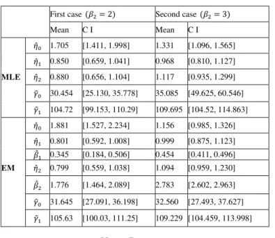
The results are stated in form of mean and a 95% confidence interval. The next table presents the estimation results:

(4)

TABLE I. SIMULATION RESULTS

First case (�₂= 2) Second case (�₂= 3)

Mean C I Mean C I

�̂0 1.705 [1.411, 1.998] 1.331 [1.096, 1.565] �̂1 0.850 [0.659, 1.041] 0.968 [0.810, 1.127] MLE �̂₂ 0.880 [0.656, 1.104] 1.117 [0.935, 1.299]

��0 30.454 [25.130, 35.778] 35.085 [49.625, 60.546] ��1 104.72 [99.153, 110.29] 109.695 [104.52, 114.863] �̂0 1.881 [1.527, 2.234] 1.156 [0.985, 1.326] �̂1 0.801 [0.592, 1.008] 0.999 [0.875, 1.123] �̂1 0.345 [0.184, 0.506] 0.454 [0.411, 0.496] EM �̂₂ 0.799 [0.559, 1.038] 1.094 [0.959, 1.230]

�̂2 1.776 [1.464, 2.089] 2.783 [2.602, 2.963] ��0 31.645 [27.091, 36.198] 32.560 [27.493, 37.627] ��1 105.63 [100.03, 111.25] 109.229 [104.459, 113.998]

V. DISCUSSION

In the long run, following the results of preceding tests, the failures process is a NHPP. The empirical cumulative distribution function of real data is evolved in the same direction as the simulated one. This process is then managed by our reliability model. Consequently, the effects of estimation show the way that there is an improvement of the system until the second failure (during 2.2 years of operation) and degradation starts from the fourth failure (beyond 8.5 years of operation). Considering the same unit of data over the improvement period and of degradation, the scale parameters

�1 and �2 over these two periods do not have a significant difference. This can be easily guaranteed with skew of an averages difference traditional test. The estimate value of �₂ is higher than 2, the failure intensity is increasing and convex announcing a marginal progress in degradation state. At the same time, �₁ takes an estimate value very near to 1 indicates that the intensity is practically constant. as a result, the failures are rather accidental and cannot be due to youth diseases. This purified model of improvement period, which is presented in

Bertholon and al. (2004), remains able independently to

concretize the hydraulic pump behavior. In light of simulations, we state the following criticisms:

• The �̂_� (�= 0,1 ou 2) have the best behavior to one side for the first case where �̂₀ appears to degrade. • The ��_� (�= 0 ou 1) are all acceptable.

• The variability of �̂_� (�= 1 ou 2) is significant enough.

As a final point , the EM procedures offer better estimators for the second case. The values of �₂ are rather higher than 2, then the curve is convex over the degradation period as it is presented in our model. A potential limitation of our model is that it involves seven parameters. In fact, it is difficult to estimate these parameters for small-sized and/or censured samples. For this reason even, the MLE appear more reliable for industrial applications.

REFERENCES

[1] A.P. Dempster, N.M. Laird and D.B. Rubin, Maximum likelihood from incomplete data via the EM algorithm. Journal. Roy. Statist. Soc. (Ser. B), 39, 1-38, 1977.

[2] Mudholkar G.S. and Srivastava D.K.. Exponentiated Weibull family for analyzing bathtub failure-rate data. IEEE Transactions on Reliability, 42, 99-102, 1993.

[3] J. Mi, Bath-tub failure rate and upside-down bathtub mean residual life. IEEE Transactions on Reliability, 44, 388-391, 1995.

[4] McLachlan G.J. and Krishnam T.. The EM algorithm and Extensions. Wiley: NewYork, 1997.

[5] T. Lim and H. Lie , Analysis of system reliability with dependent repair modes. IEEE Transactions on Reliability 49, 153–162, 2000.

[6] M. Xie, Y. Tang and T.N. Goh, A modified Weibull extension with bathtub-shaped failure rate function. Reliability Engineering and System Safety, 76, 3, 279-290, 2002.

[7] Y. Lefebvre, Using the Phase Method to Model Degradation and Maintenance Efficiency. International Journal of Reliability, Quality and Safety Engineering, 10, 4, 383-405, 2003.

[8] H. Langseth, and B. Lindqvist, A maintenance model for components exposed to several failure mechanisms and imperfect repair, In: Doksum, K., Lindqvist, B. (Eds.), Mathematical and Statistical Methods in Reliability. In: Quality, Reliability and Engineering Statistics, World Scientific Publishing Co., pp. 415–430, 2003.

[9] H. Langseth, and B. Lindqvist, A maintenance model for components exposed to several failure mechanisms and imperfect repair, In: Doksum, K., Lindqvist, B. (Eds.), Mathematical and Statistical Methods in Reliability. In: Quality, Reliability and Engineering Statistics, World Scientific Publishing Co., pp. 415–430, 2003.

[10] H. Bertholon, N. Bousquet and G. Celeux, An alternative competing risk model to the Weibull distribution in lifetime data analysis. Technical Report : RR-5265, INRIA Press, Orsay, France, 2004.

[11] E.A. Peña, E.H. Slate, and J.R. González, Semi-parametric inference for a general class of models for recurrent events, J Stat Plan Inference 137, 1727–1747, 2007.

[12] J. Sethuraman and M. Hollander, Non-parametric bayes estimation in repair models, Journal of Statistical Planning and Inference 139, 1722-1733, 2009.

[13] P. Basak, I. Basak and N. Balakrishnan, Estimation for the three-parameter lognormal distribution based on progressively censored data, Computational Statistics and Data Analysis 53, 3580-3592, 2009. [14] Y. Dijoux, A virtual age model based on a bathtub shaped initial intensity,

Reliability Engineering and System Safety, vol. 94, pp 982-989, 2009. [15] M. Franco, J. M. Vivo and N. Balakrishnan, Reliability properties of

generalized mixtures of Weibull distributions with a common shape parameter, Journal of Statistical Planning and Inference 141, 2600-2613, 2011.

[16] L. Doyen, On the Brown-Proschan model when repair effects are unknown, Applied Stochastic Models in Business and Industry 27, 600-618, 2011.

[17] G. Babykina and V. Couallier, Empirical assessment of the maximum likelihood estimator quality in a parametric counting process model for recurrent events, Computational Statistics and Data Analysis 56, 297– 315, 2012.

[18] L. Doyen, Reliability analysis and joint assessment of Brown-Proschan preventive maintenance efficiency and intrinsic wear-out, Computational Statistics and Data Analysis 56, 4433-4449, 2012

[19] M. Krit and A. Rebai, An estimate of maintenance efficiency in Brown-Proschan imperfect repair model with bathtub failure intensity, Journal of Industrial Engineering and Management, Vol 5, No 1, 88-101, 2012.

[20] M. KRIT and A. REBAI, Modeling of the Effect of Corrective and Preventive Maintenance with Bathtub Failure Intensity, International Journal of Technology, 2: 157-166, 2013.

[21] M. Krit, Generalized Dependent Competing Risks for Imperfect Maintenance, International Journal of Industrial and Systems Engineering, Vol. 18, No. 4, 454-466, 2014.

[22] I. Dewan and Y. Dijoux, Modelling repairable systems with an early life under competing risks and asymmetric virtual age, 144, 215–224, (2015).