Analysis of the Weekend Effect on the Markets of 121 Equity Indices and 29 Commodities

(1)

EURASIAN JOURNAL OF BUSINESS AND

MANAGEMENT

http://www.eurasianpublications.com

23

ANALYSIS OF THE WEEKEND EFFECT ON THE MARKETS OF 121 EQUITY

INDICES AND 29 COMMODITIES

Krzysztof Borowski

Warsaw School of Economics, Poland. Email: [email protected]

Abstract

The problem of efficiency of financial markets, especially the weekend effect has always fascinated scientists. The issue is significant from the point of view of assessing the portfolio management effectiveness and behavioral finance. This paper tests the hypothesis of weekend effects of the market of 121 equity indices and 29 commodities with the following four approaches: Friday close – Monday open, Friday close – Monday close, Friday close – Tuesday open and Friday close – Tuesday close prices. Calculations presented in this paper indicate the presence of the monthly effect in the following cases: 36 (I approach), 58 (II approach), 57 (III approach) and 66 (IV approach).

Keywords: Market Efficiency, Commodity Market, Equity Market, Calendar Anomalies

1. Introduction

Efficient market hypothesis (EMH), the core of the influential paper of Fama (1970), has been a cornerstone of financial economics for many decades. Although current definitions differ from that developed by Fama, the efficiency of markets prevents systematic beating of the market, usually in a form of above-average risk-adjusted returns. The problem ofthe financial markets efficiency, especially of equity markets, has been discussed ina number ofacademic works, which has led to a sizable set of publications examining this subject. In many empirical works dedicated to the time series analysis of rates of return and stock prices, there were found statistically significant effects of both types, i.e. calendar effects and effects associated with the size of companies. These effects are called anomalies, because their existence testifies against market efficiency. Discussion of the most common anomalies in the capital markets can be found, among others, in Simson (1988) or Latif et al. (2011).

One of the most common calendar anomalies observed on the financial markets are:

a) Day-of-the-week effect – daily average rates of return registered on the stock market differ

(2)

24

day-of-the-week effect in the US market was also presented, among others, in the works of Jaffe et al. (1989), French (1980), and Lakonishok and Maberly (1990). The evidence for UK market was examined by Theobald and Price (1984), Jaffe and Westerfield (1985), Board and Sutcliffe (1988), Agrawal and Tandon (1994), Peiro (1994), Mills and Coutts (1995), Dubois and Louvet (1996), and Coutts and Hayes (1999). Peiro (1994),Agrawal and Tandon (1994), Dubois and Louvet (1996) and Kramer (1996) provided evidence of negative Monday and Tuesday returns for Frankfurt exchange. In works of Solnik and Bousquet (1990), and Agarwal and Tandon (1994), there was found an evidence of negative Tuesday rates of return in Paris market, while Condoyanni et al. (1987) and Peiro (1994) demonstrated negative Monday and Tuesday rates or return on the same market and Barone (1990) in Milan. Research regarding the rates of return on other market was performed in the work of Kato et al. (1990), and also by Sutheebanjard and Premchaiswadi (2010). Islam and Sultana (2015) proved for the CASPI Index (Chittagong Stock Exchange) that the day-of-the-week effects on stock returns and volatility are persistent in the stock market.

b) Monthly effect– achieving by portfolio replicating the specified stock index, different returns in each month. The most popular monthly effect is called “January effect”, i.e. the tendency to observe higher average rate of return of stock market indices in the first month of the year. For the first time, this effect was observed by Keim (1983), who noted that the average rate of return on stocks with small capitalization is highest in January. In case of large and mid-capitalization companies the effect was not so perceptible. Although January was the best single month in UK, the period from December to April consisted of months, which on average produced positive returns (Rozeff and Kinney, 1976; Corhay et al. 1988). Bernstein (1991), taking into consideration the behavior of the US equity market in the period from 1940 to 1989, discovered the interdependence between rates of returns in each month. Modern researches, e.g. Gu (2003) and Schwert (2002) proved that in the last two decades of the twentieth century, phenomenon of the month-of-the-year effect was much weaker. This fact would suggest that the discovery and dissemination of the monthly effect in world financial literature contributed to the increase of market efficiency.

c) Other seasonal effects– the following calendar effects can be found in the financial literature:

1. The weekend effect – Cross (1973) found that markets tend to rise on Fridays and fall on Mondays. His findings generated a flood of research (Lakonishok and Levi, 1982; Jaffe and Westerfield, 1985; Condoyanniet al. 1987; Connolly, 1991; Coutts and Hayes, 1999). In the literature two ways of computing weekend rates of return are implemented. In the first, Friday close and Monday open prices are used, while in the second Friday close and Monday close prices are employed.

2. The holiday effects – markets before holidays or other trading breaks tend to rise. In the US there are a number of studies looking at this, e.g., Fields (1934), Ariel (1987; 1990), Lakonishok and Smidt (1988) and Cadsby and Ratner (1992).

3. Within-the-month effect– positive rates of returns only occur in the first half of the month (Ariel, 1987; Kim and Park,1994).

4. Turn-of-the month effect – average rate of return calculated for the last day of the month and for three days of the next month, was higher than the average rate of return calculated for the month, for which the rate of return of only one session, was taken (Cadsby and Ratner, 1992). Lakonishok and Smidt (1988) found that the four days at the turn-of-the-month averaged a cumulative rate of increase of 0.4730% versus 0.0612% for and average four days. The average monthly increase was 0.3490%, i.e., the DJIA went down during non-turn-of-the-month period.

(3)

25

and (4) Friday close – Tuesday close. Prices of commodities quotations are taken from the Reuters.

2. Literature Review

The earliest study of day-of-the-week effect was made by Fields (1934), who found that the US market tended to rise on Saturdays (the market used to open for a couple of hours on Saturdays). Cross (1973) discovered the Fridays rates of return were positive, while on Mondays were negative. His findings generated a flood of research reporting so called “Blue Monday” effect with rates of return endeavoring to be higher at the end of the trading week (Lofthouse, 1994; Lakonishok and Smidt, 1988).

French (1980) noted that the average return of the SP 500 was reliably negative over weekends in the period 1953–1977. His observations were confirmed by Schwert (2002) and Keim and Stambaugh (1984).

The weekend effect was also examined for countries different than US (Jaffe and Westerfield, 1985; Condoyanni et al. 1987). Board and Sutcliffe (1988) found evidence of the weekend effect in the UK in the period of 1962-1986. According to Choy and O’Hanlon (1989) the day-of-the-week effect seemed to be stronger on the UK market than in the US. Kamara (1997) proved that the weekly effects declined in the period of 1962-1993 because of increased institutional trading in large cap stocks. His result were confirmed by Steeley (2001), who revealed that the weekend effect disappeared in the 1990s.

Ziemba (1993) found that Fridays average rates of return were positive and Mondays negative when the session on Friday was the last session in the week, while the average rates of return on Sundays were highly positive in the weeks with Saturday trading.

According to Chen and Singal (2003) the Fridays increase and Mondays falls of prices were caused by covering short position and opening new ones, respectively. Chan et al. (2004) argued that Monday negative rates of return were due to the individual not institutional investors - the Monday average return was the same as on the other four sessions in the week for equities with high institutional holdings.

Branch and Ma (2006) analyzing socks quoted on the NYSE, AMEX and Nasdaq in the period of 1994-2005 and breaking them into six categories, found a strong negative autocorrelation between the overnight return (e.g. between the market close and its opening the next working day) and the intraday returns. According to the authors the cause of the anomaly was related to the following factors: market makers’ behavior, strategies implemented by market specialist and expectations of the next session opening prices regarding their assigned stock.

Cooper et al. (2008) demonstrated that the US equity premium in the period of 1993-2006, for stocks characterized by intraday return close to zero, was a result of overnight returns. According to them the majority of analyzed stock returns quoted on NYSE, AMEX, Nasdaq and Chicago Mercantile Exchange, was generated when the market was close and the difference between night and daily return was between 2,61 and 7,61 basis points per day.

Stoll and Whaley (1990) reported that open-to-open returns are more volatile than close-to-close returns. Wang et al. (2009) investigated that the two components of the total daily return (closet– closet+1), the overnight return (closet– opent+1), and the intraday return (opent –

closet) for 2215 NYSE stocks in the period of 1988-2007 tended to be auto-correlated and found

thatthe cross correlations between the three different returns (total, overnight and intraday) were quite stable over the entire 20 year period for the NYSE stocks.

3. Data and Methods

The research is divided into four parts. The calculation were proceeded concerning 121 world stock indices and 29 commodities – in the parenthesis are indicated the first month and year considered in the process of rates of return calculation.

(4)

26

20 (02.01.1992), BELEX 15 (04.10.2005), BET (31.10.2000), BUMIX (01.06.2004), BUX (02.01.1991), BOVESPA (12.07.1989), CAC40 (08.01.1965), CASA ALL Shares (02.01.2002), CDAX (15.03.2004), CNX NIFTY (03.11.1995), CNX NIFTY TR (17.09.2007), CRB (03.01.1994), CROBEX (19.10.2009), CSE ALL Shares (06.06.1994), CSI 300 (08.04.2005), CYMAIN (06.09.2004), DAX (28.09.1959), DF MAIN (31.12.2003), DJ Composite (23.12.1980), DJ Eurostoxx (08.08.2002), DJIA (02.01.1900), DJTA (02.01.1900), DJUA (02.01.1929), EGX 30 (01.01.1998), EGX 70 (01.03.2009), EGX 100 (02.01.2006), EOE (01.02.1995), ESTX 50 PR (31.12.1986), ESTX PR (23.02.1998), EURONEXT 100 (15.03.2001), FTSE 100 (22.10.1992), FTSE 250 (30.12.1985), FTSE EUROTOP 100 (20.11.1990), FTSEMIB (01.02.1998),FTSEurofirst 300 (28.07.1997), HANG SENG (24.11.1969), HEX (02.01.995), HSCE (01.08.1994), IBEX (05.01.1987), ICEX (31.12.1992), IGBC (27.11.2001), IPC (08.11.1991), IPSA (02.01.1987), ISEQ (19.02.1992), JCI (04.04.1983), JKSE (20.07.1995), KARACHI 100 (25.05.1994), KLCI (03.01.1977), KLSE (13.04.1992), KOSPI (04.01.1980), KW MAIN (05.03.1997), KW WEIGHTED IDW (26.01.2009), LIMA GENERAL (09.02.1995), MDAX (29.02.1996), MERVAL (04.04.1988), MICEX (22.09.1997), MSCI AC WORLD (14.07.2003), MSCI WORLD (14.07.2003), MSE (27.12.1995), MSM MAIN 30 (01.01.1992), mWIG40 (31.12.1997), NASDAQ (03.01.1938), NASDAQ 100 (01.10.1985), NEXT 150 IDX (13.03.2001), NIKKEI (01.03.2014), NSE ALL Shares (14.01.2000), NZX 50 (03.01.2001), OBX (07.09.1999), OMX Riga (03.01.2001), OMX Stockholm (30.09.1986), OMX Talin (03.01.1980), OMX Vilnius (01.01.2001), OSE (03.01.1983), PFTS (25.08.1998), PLE MAIN (11.02.1997), PSEI (02.01.1986), PSI20 (31.12.1992), PX (03.09.1993), QE MAIN 20 (10.08.1998), RTS (01.09.1995), RUSSEL (04.03.1999), SAX (03.07.1995), SBITOP (04.04.2006), SDAX (15.03.1999), SESESLCT (02.01.2003), SENSEX (03.04.1979), SET (02.07.1987), SMI (01.07.1988), SOFIX (26.11.2001), SP 500 (02.01.1900), SP ASX 200 (03.04.2000), SP TSX Composite (03.01.1961), SSE B-Shares (04.01.2000), SSE Composite (19.12.1990), Straits Times (28.12.1987), STXE 50 (23.02.1998), STXE 600 (23.02.1998), sWIG80 (29.12.1994), TAIEX (05.01.1995), TASE MAIN 100 (08.10.1992), TECDAX (16.09.1999), TDW MAIN (19.10.1998), TOPIX (02.04.1990), TSE 300 (15.08.1989), TUN MAIN Index (31.12.1997), TWII (12.03.1992), UK 100 (13.11.1935), UX (03.11.1997), VNI (28.07.2000), WIG (16.04.1991), WIG20 (14.04.1994), XU 30 (02.01.1997), XU 100 (02.01.1990).

The CRB index is a commodity index but as an index was classified to the group of the equity indices.

Commodities (in brackets the date of the first quotation included in the analysis): Brent oil (30.03.1983), canola (01.09.1998), cocoa (01.07.1959), coffee (17.08.1973), copper (01.07.1969), corn (01.01.1967), cotton (01.07.1959), crude oil (30.09.1983), feeder cattle (06.09.1973), gas oil (01.09.1998), gasoline (01.09.1998), gold (02.06.1969), heating oil (06.03.1979), lean hogs (25.06.1969), live cattle (05.01.1970), lumber (01.09.1998), natural gas (03.04.1990), orange juice (01.02.1967), palladium (05.01.1977), platinum (01.03.1968), rubber (23.01.1990), silver (13.06.1963), rough rice (01.09.1998), soybean (01.07.1959), soybean meal (01.09.1998), soybean oil (01.09.1998), sugar (04.01.1961), wheat (01.07.1959), wheat KCBT (01.09.1998) – data form Reuters service.

For both stock indices and commodities the last session considered in the process of calculating rates of return was 30.06.2015.

The adapted methodology in the paper can be divided into:

1. Testing the null hypothesis regarding equality of variances of rates of return in two populations,

(5)

27

3.1. Testing the Null Hypothesis Regarding Equality of Variances of Rates of Return in Two Populations

The null and alternative hypothesis can be formulated as follows:

�

0 :�12=�22 �

1 :�12≠ �22 (1)

where:

�12- variance of rates of returnin the first population, �22- variance of rates of returnin the second population.

As the last part of the calculation will be carried out using the F-statistics (so called Fisher-Snadecor statistics) for equality of variances of two population rates of return, where = �2

�2, with the condition that: �

2_>_�2_{and the degrees of freedom are equal:} � –for variance in the numerator of F,

� –for variance in the denominator of F.

If test (computed for α=0,05) is lower than statistics, e.g. the ratio test to F-statistics is lower than 1, there is no reason to reject the null hypothesis.

3.2. Testing the Null Hypothesis Regarding Equality of Average Rates of Returns in Two Populations

According to the adopted methodology, the survey covers two populations ofreturns, characterized by normal distributions. On the basis of two independent populations of rate of returns, which sizes are equal n1 and n2, respectively, the hypotheses H0 and H1 should be

tested with the use of statistics z (Osinska, 2006, pp.43-44):

z = r1 −r2 S 1_{n 1}2+S 2

2

n 2

(2)

where:

�1–average rate of return in the first population, �2–average rate of return in the second population.

The Formula 2 can be used in case of normally distributed populations, when the population variances are unknown but assumed equal. The number of degrees of freedom is equal to: ��(1) =�1+�2−2.

When the population variances are unequal, the number of degrees should be modified according to the following formula (Defusco et al. 2001, p.335):

��(2) =

�12 �1+

�22 �2

2

�12 �1 2

�1 + �22 �2

2

�2

(3)

(6)

28

�₀: �₁ = �₂

�1: �1 ≠ �2 (4)

In particular:

1. For the analysis of the overnight rates of return for individual days of the week, if�₁ is the overnight average rate of return on day Y (the first population), then �₂ is the overnight average rate of return in all other days, except day Y (the second population). 2. For the analysis ofthe one-session rates of return for individual days of the week, if�₁ is the one-session average rate of returnon day Y (the first population), then �₂ is the one-session average rate of return in all other days, except day Y (the second population).

In all analyzed cases, the p-values will be calculated with the assumption that the populations variances are unknown, but:

1. population variances are assumed equal–p-value(1), 2. population variances are assumed unequal–p-value(2).

In case, when there is no reason to reject the null hypothesis about equality of variances of two observed returns, the p-value(1) should be compared with the critical value 0,05; otherwise the p-value(2) will be used - that explains the reason of applying p-value in the following part of the paper. If thep-value (p-value(1) or p-value(2)) is less than or equal to0,05; then the hypothesis H0 is rejected in favor of the hypothesis H1. Otherwise, there is no reason to reject hypothesis H0. In the part 3 of the paper, the value listed in the tables are equal to p-value(1) or p-value(2) depending on the result of testing the null hypothesis, concerning the equality of variance in two populations of rates of returns.

In the first part, the test for equality of two overnight average rates of return will be exemplified for rates of return in two populations. Assuming, that if the first population is composed of the rates of return calculated for Friday close and Monday open prices, then the second population determines the overnight rates of return for all remaining overnight rates of return. Whilethe sessionswere also heldon Saturdaysweekendrates of returnwere calculatedas follows:Saturdayclose-Mondayopen. In case of the Islamic countries the Thursday close and Sunday open prices have been taken into account.

In the second part, the test for equality of two one-session average rates of return will be exemplified for rates of return in two populations. Assuming, that if the first population is composed of the daily rates of return calculated for Friday close and Monday close prices, then the second population determines the one-session rates of return for all remaining daily rates of return (with an appropriate adjustmentwhilesessionswere held on Saturdays in the analyzed period). In case of the Islamic countries the Thursday close and Sunday close prices will be applied.

In the third part, the test for equality of two average rates of return will be exemplified for rates of return in two populations. Assuming, the if the first population is composed of the daily rates of return calculated for Friday close and Tuesday open prices, then the second population determines the one-session plus overnight rates of return for all remaining rates of return (with an appropriate adjustmentwhilesessionswere held on Saturdays in the analyzed period). In case of the Islamic countries the Thursday close and Monday open prices will be applied.

(7)

29

4. Analysis of Results

4.1. Analysis of the Weekend Effect: Friday Close – Monday Open

The results of testing zero hypothesis with the use of average rates of returns for two different populations permit to draw following conclusions:

1. The null hypothesis regarding equality of variances of daily average rates of return in two populations, was rejected (for α=5%) in the following 130 cases: AEX, ALL ORDINARIES, ALSIUG, AMEX, AMM FR FLT, ATHEX, ATX, BEL 20, BELEX 15, BET, BOVESPA, BUMIX, BUX, CAC40, CDAX, CNX NIFTY TR, CRB, CROBEX, CSE ALL Shares, CYMAIN, DAX, DF MAIN, DJ Composite, DJ Eurostoxx, DJIA, DJTA, DJUA, EGX 30, EGX 70, EGX 100, EOE, ESTX PR, ESTX 50 PR, EURONEXT 100, FTSE 100, FTSE 250, FTSE EUROTOP 100, FTSEMIB, FTSEurofirst, HEX, HANG SENG, IBEX, ICEX, IGBC, IPC, IPSA, ISEQ, JCI, JKSE, KLCI, LIMA GENERAL, mWIG40, MDAX, MERVAL, MICEX, MSCI AC WORLD, MSE, MSM MAIN 30, NASDAQ, NASDAQ 100, NEXT 150 IDX, NIKKEI, NSE ALL Shares, NZX50, OMX Stockholm, OMX Talin, OMX Vilnius, OSE, PFTS, PLE MAIN, PSEI, PX, QE MAIN 20, RTS, RUSSELL, SASESLCT, SAX, SDAX, SENSEX, SET, SBITOP, SMI, SP 500, SP TSX Composite, SSE B-Shares, SSE Composite, Straits Times, STXE 50, sWIG80, TAIEX, TASE MAIN 100, TDW MAIN, TOPIX, TSE 300, TUN MAIN Index, TWII, UK 100, UX, VNI, WIG, WIG20, XU 30, XU 100, Brent oil, canola, cocoa, coffee, copper, corn, cotton, crude oil, feeder cattle, gasoline, gold, heating oil, lean hogs, live cattle, lumber, natural gas, orange juice, palladium, platinum, rubber, silver, soybean, soybean meal, soybean oil, sugar, wheat, wheat KCBT.

2. The null hypothesis regarding equality of two average rates of return was rejected for the following 36 indices and commodities (p-value shown in parenthesis): AEX (0.0025), ALSIUG (0.0096), CAC40 (0.0012), CRB (0.0023), DAX (0.0001), DJ Composite (0.0007), DJ Eurostoxx (0.0418), DJIA (0.0036), DJTA (0.0001), DJUA (0.0001), EGX 30 (0.0002), FTSE 250 (0.0010), HANG SENG (0.0183), IPSA (0.0001), ISEQ (0.0001), KLCI (0.0001), KW MAIN (0.0028), MERVAL (0.0005), NASDAQ (0.0001), NIKKEI (0.0001), PSEI (0.0481), QE MAIN 20 (0.0001), SDAX (0.0014), SET (0.0216), SMI (0.0466), SP 500 (0.0001), SP TSX Composite (0.0001), Straits Times (0.0047), sWIG80 (0.0087), XU 100 (0.0743), copper (0.0002), corn (0.0021), cotton (0.0263), palladium (0.0396), platinum (0.0046), rubber (0.0257).

In all other cases, there was no reason to reject the null hypothesis in favor of the alternative hypothesis but the p-value higher than 0.05 and lower than 0.1 was registered in the following cases: BET (0.0924), BOVESPA (0.0900), ESTX 50 PR (0.0581), MSE (0.0852), PLE MAIN (0.0566), cocoa (0.0605).

4.2. The Analysis of the Weekend Effect: Friday Close – Monday Close

(8)

30

IDX, NIKKEI, NSE ALL Shares, OBX, OMX Stockholm, OMX Talin, OMX Vilnius, OSE,PFTS, PLE MAIN, PSEI, PSI 20, PX, QE MAIN 20,RTS, RUSSELL, SASESLCT, SAX, SDAX, SENSEX, SET, SMI, SOFIX, SP 500, SP ASX 200, SP TSX Composite, SSE B-Shares, Straits Times, STXE 50, STXE 600, sWIG80, TAIEX, TASE MAIN 100, TECDAX, TOPIX, TSE 300, TUN MAIN Index, TWII, UK 100, UX, VNI, WIG, XU 30, XU 100, Brent oil, canola, cocoa, coffee, corn, cotton, crude oil, gold, heating oil, live cattle, lean hogs, lumber, natural gas, orange juice, platinum, rubber, silver, soybean, soybean meal, soybean oil, sugar, wheat, wheat KCBT.

2. The null hypothesis regarding equality of two average rates of return was rejected for the following 58 indices and commodities (p-value shown in parenthesis): ALSIUG (0.0095), BET (0.0366), BOVESPA (0.0026), CAC40 (0.0082), CNX NIFTY (0.0002), CRB (0.0030), CROBEX (0.0001), CSI 300 (0,0001), CSE ALL Shares (0.0006), CYMAIN (0.0108), DAX (0.0002), DJ Eurostoxx (0.0335), DJIA (0.0001), DJTA (0.0001), DJUA (0.0001), EGX 70 (0.0435), EGX 100 (0.0032), FTSE 250 (0.0002), HANG SENG (0.0078), HSCE (0.0001), ICEX (0.0188), IPC (0.0083), IPSA (0.0001), JCI (0.0403), JKSE (0.0001), KARACHI 100 (0.0177), KLCI (0.0001), KLSE (0.0003), MERVAL (0.0001), NASDAQ (0.0001), NIKKEI (0.0001), OMX Riga (0.0032), PLE MAIN (0,0231), PSEI (0.0051), QE MAIN 20 (0.0003), SASESLCT (0.0004), SET (0.0001), SP 500 (0.0001), SP ASX 200 (0.0001), SP TSX Composite (0.0001), Straits Times (0.0001), TAIEX (0.0065), TOPIX (0.0127), XU 30 (0.0110), XU 100 (0.0068), Brent oil (0.0006), cocoa (0.0002), copper (0.0001), cotton (0.0277), crude oil (0.0403), gasoline (0.0001), gold (0.0242), heating oil (0.0003), lumber (0.0298), palladium (0.0250), platinum (0.0014), silver (0.0160), sugar (0.0056).

In all other cases, there was no reason to reject the null hypothesis in favor of the alternative hypothesis but the p-value higher than 0.05 and lower than 0.1 was registered in the following cases: BELEX 15 (0.0810), BUX (0.0918), MSE (0.0832), NASDAQ (0.0936), OSE (0.0737), TUN MAIN Index (0.0698), TWII (0.0854), VNI (0.0846), gas oil (0.0761), soybean (0.0647).

4.3. The Analysis of the Weekend Effect: Friday Close – Tuesday Open

1. The null hypothesis regarding equality of variances of daily average rates of return in two populations, was rejected (for α=5%) in the following 113cases: ADX, AEX, ALL ORDINARIES, ALSIUG, AMEX, AMM FR FLT, ATX, BEL 20, BELEX 15, BOVESPA, BUX, CASA ALL Shares, CDAX, CRB, CROBEX, CSE ALL Shares, CYMAIN, DAX, DF MAIN, DJ Composite, DJ Eurostoxx, DJTA, DJUA, EGX 30, EGX 70, EOE, ESTX PR, ESTX 50 PR, EURONEXT 100, FTSE 100, FTSE 250, FTSE EUROTOP 100, FTSEurofirst, FTSEMIB, HEX, ICEX, IGBC, IPC, IPSA, JCI, KARACHI 100, KLCI, KLSE, KOSPI, KW MAIN, LIMA GENERAL, MDAX, MERVAL, MSCI AC WOLRD, MSCI WORLD, MSE, MSM MAIN 30, NEXT 150 IDX, NIKKEI, NSE ALL Shares, NZX50, OBX, OMX Stockholm, OMX Talin, OMX Vilnius, OSE, PFTS, PLE MAIN, PSEI, PSI 20, PX, QE MAIN 20, RTS, RUSSELL, SASESLCT, SDAX, SMI, SOFIX, SP 500, SSE B-Shares, SSE Composite, SP TSX Composite, Straits Times, STXE 50, STXE 600, sWIG80, TAIEX, TASE MAIN 100, TECDAX, TOPIX, TSE 300, TWII, UK 100, UX, WIG, WIG20, XU 30, XU 100, Brent oil, coffee, copper, corn, cotton, crude oil, gas oil, heating oil, lean hogs, live cattle, natural gas, orange juice, palladium, rubber, silver, soybean, soybean meal, sugar, wheat, wheat KCBT.

(9)

31

DJUA (0.0001), FTSE 250 (0.0015), HANG SENG (0.0004), ICEX (0.0334), IGBC (0.0001), IPC (0.0082), IPSA (0.0001), JCI (0.0001), JKSE (0.0001), KARACHI 100 (0.0067), KLCI (0.0001), KLSE (0.0010), MERVAL (0.0003), MSE (0.0418), NASDAQ (0.0001), NIKKEI (0.0001), OMX Riga (0.0224), PSEI (0.0007), PLE MAIN (0.0042), SASESLCT (0.0003), SENSEX (0.0118), SET (0.0001), SP 500 (0.0001), SP TSX Composite (0.0001), SSE Composite (0.0316), Straits Times (0.0001), TAIEX (0.0030), TOPIX (0.0008), TUN MAIN Index (0.0096), TWII (0.0122), WIG (0.0413), VNI (0.0013), XU 30 (0.0108), XU 100 (0.0068), Brent oil (0.0003), cocoa (0.0002), copper (0.0001), crude oil (0.0101), gas oil (0.0001), gasoline (0.0001), gold (0.0187), heating oil (0.0011), lumber (0.0002), palladium (0.0172), platinum (0.0007), silver (0.0010), sugar (0.0014).

The p-value higher than 0.05 and lower than 0.1 was registered in the following cases: ATHEX (0.0826), BET (0.0536), EGX 70 (0.0662), MDAX (0.0916), OSE (0.0507), PSI 20 (0.0934), SBITOP (0.0691), SMI (0.0643), lean hogs (0.0612), live cattle (0.0778).

4.4. The Analysis of the Weekend Effect: Friday Close – Tuesday Close

1. The null hypothesis regarding equality of variances of daily average rates of return in two populations, was rejected (for α=5%) in the following 75 cases: ADX, ALL ORDINARIES, ALSIUG, AMM FR FLT, BELEX 15, BOVESPA, BUMIX, BUX, CDAX, CNX NIFTY, CROBEX, RB, CSI 300, CYMAIN, DAX, DJIA, DJTA, DJUA, ESTX 50 PR, EURONEXT 100, HANG SENG, HEX, HSCE, ICEX, IGBC, JCI, JKSE, KLCI, KLSE, KOSPI, KW WEIGHTED IDW, MERVAL, MSE, MSM MAIN 30, NIKKEI, NSE ALL Shares, OMX Stockholm, OMX Talin, OMX Vilnius, PFTS, PLE MAIN, PX, QE MAIN 20, RUSSELL, SASESLCT, SENSEX, SBITOP, SOFIX, SP 500, SP ASX 200, SP TSX Composite, SSE Composite, Straits Times, sWIG80, TDW MAIN, TECDAX, TOPIX, TSE 300, UX, WIG, WIG20, XU 30, coffee, copper, corn, gas oil, gasoline, lean hogs, live cattle, natural gas, orange juice, palladium, platinum, soybean, soybean meal. 2. The null hypothesis regarding equality of two average rates of return was rejected for

the following 66 indices and commodities (p-value shown in parenthesis): ALSIUG (0.0048), AMM FR FLT (0.0427), ATHEX (0.0421), ALL ORDINARIES (0.0207), AMEX (0.0318), BELEX 15 (0.0096), BET (0.0228), BOVESPA (0.0368), CAC40 (0.0012), CRB (0.0104), CROBEX (0.0003), CSE ALL Shares (0.0001), CYMAIN (0.0345), DAX (0.0004), DJIA (0.0009), DJTA (0.0001), DJUA (0.0001), FTSE 250 (0.0006), HANG SENG (0.0005), ICEX (0.0039), IGBC (0.0005), IPSA (0.0234), JCI (0.0001), JKSE (0.0001), KARACHI 100 (0.0371), KLCI (0.0001), KLSE (0.0065), KW MAIN (0.0015), MDAX (0.0344), MERVAL (0.0007), MSE (0.0409), NIKKEI (0.0001), NASDAQ (0.0001), OMX Riga (0.0122), OSE (0.0282), PLE MAIN (0.0026), PSEI (0.0001), SASESLCT (0.0022), SENSEX (0.0165), SET (0.0001), SBITOP (0.0039), SOFIX (0.0439), SP 500 (0.0001), SP TSX Composite (0.0001), SSE Composite (0.0180), Straits Times (0.0001), TAIEX (0.0018), TOPIX (0.0138), TUN MAIN Index (0.0011), TWII (0.0026), VNI (0.0003), WIG (0.0334), XU 30 (0.0017), XU 100 (0.0068), Brent oil (0.0001), cocoa (0.0334), copper (0.0001), crude oil (0.0026), gas oil (0.0219), gasoline (0.0001), heating oil (0.0007), lean hogs (0.0107), live cattle (0.0056), lumber (0.0001), platinum (0.0135), silver (0.0115), sugar (0.0003).

The p-value higher than 0.05 and lower than 0.1 was registered in the following cases: CSI 300 (0.0852), HSCE (0.0669), IPC (0.0612), LIMA GENERAL (0.0654), mWIG40 (0.0798), sWIG80 (0.0981), TSE 300 (0.0603), cotton (0.0568), feeder cattle (0.0929), soybean (0.0919).

(10)

32

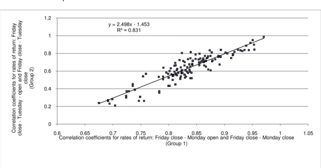
2. Group 2: Friday close – Tuesday open and Friday close – Tuesday close

It has been confirmed strong dependence between correlation coefficients in these two groups – see Figure 1. Dependence between correlation coefficient in the Group 2 (y) and the correlation coefficient in Group 1 (x) is described with the following equation:

= 2,4985∙ −1,4534 (5) The R2 is equal to 0.831.

Figure 1. Linear Regression for Correlation Coefficients in Group 1 and Group 2

5. Conclusion

The aim of this study was to determine the prevalence of the weekend effect on the markets of 121 equity indices and 29 commodities. Analysis of the effects of seasonality included an examination of the rates of return calculated for four approaches:

1. Friday close – Monday open prices, 2. Friday close – Monday close prices, 3. Friday close – Tuesday open prices, 4. Friday close – Tuesday close prices.

Calculations presented in this paper indicate the presence of the weekend effect in the following cases: 36 (I approach), 58 (II approach), 57 (III approach) and 66 (IV approach). The existence of seasonality effects occurred in both developedandemergingstock marketsas well as on the commodity markets. The weekend effect, in its modified version, was also observed in the Islamic countries. In case of 20 equity indices and commodities, the weekend effect was observed for all four approaches (ALSIUG, CAC40, CRB, DAX, DJIA, DJTA, DJUA, FTSE 250, HANG SENG, IPSA, KLCI, MERVAL, NASDQAQ, NIKKEI, PSEI, SET, SP 500, Straits Times, copper, platinum). For all three remaining approaches, the number of the indices and commodities observed in each of them was equal to: 22, 19 and 33, respectively. The weekend effect was observed in three out of four approaches for the following indices: BOVESPA, CROBEX, CYMAIN, ICEX, JCI, JKSE, KARACHI, KLSE, OMX Riga, PLE MAIN, SASESLCT, TAIEX, TOPIX, XU 100, Brent oil, cocoa, crude oil, gasoline, heating oil, palladium, silver, and sugar.

The main limitation of this research is the assumption of normal distribution of return rates of analyzed indices and commodities along with the use of price data gained from Reuters

y = 2.498x - 1.453 R² = 0.831

0 0.2 0.4 0.6 0.8 1 1.2

0.6 0.65 0.7 0.75 0.8 0.85 0.9 0.95 1 1.05

Cor re lat ion co e ff ici e n ts fo r ra te s o f re tu rn : F rida y close -T u e sd a y -o p e n a n d F rida y close -T u e sd a y close (Gr o u p 2 )

(11)

33

data source as well as the unequal intervals of observations for different equity indices and commodities.

The outcome may be regarded as a part of the ongoing discussions on the hypothesis of financial markets efficiency, which was introduced by Fama (1970).

Results obtained in the paper regarding the weekend effect on the gold market are consistent with those of French (1980), Schwert (1990), Keim and Stambaugh (1984), and Board and Sutcliffe (1988). Further research onthe occurrence of weekend anomalies in the financial markets should cover the currency market.

References

Agrawal, A. and Tandon, K., 1994. Anomalies or illusions? Evidence from stock markets in eighteen countries. Journal of International Money and Finance, 13, pp.83-106. http://dx.doi.org/10.1016/0261-5606(94)90026-4

Ariel, R., 1987. A monthly effect in stock returns. Journal of Financial Economics, 17, pp.161-174. http://dx.doi.org/10.1016/0304-405X(87)90066-3

Ariel, R., 1990. High stock returns before holidays: Existence and evidence on possible causes. Journal Finance, 45, pp.1611-1626. http://dx.doi.org/10.1111/j.1540-6261.1990.tb03731.x

Barone, E., 1990. The Italian stock market: Efficiency and calendar anomalies. Journal of Banking and Finance, 14, pp.493-510. http://dx.doi.org/10.1016/0378-4266(90)90061-6 Bernstein, J., 1991. Cycles of profit. New York: Harpercolins.

Board, J. and Sutcliffe, C. 1988. The weekend effect in UK stock market returns. Journal of Business, Finance & Accounting, 15, pp.199-213. http://dx.doi.org/10.1111/j.1468-5957.1988.tb00130.x

Branch, B. and Ma, A., 2006. The overnight return, one more anomaly. Working Paper. [online] Available at: <http://ssrn.com/abstract=937997> [Accessed 15 July 2015].

Cadsby, C. and Ratner, M., 1992. Turn-of-month and pre-holiday effects on stock returns: Some international evidence. Journal of Banking and Finance, 16, pp.497-509. http://dx.doi.org/10.1016/0378-4266(92)90041-W

Chan, S., Leung, W., and Wang, K., 2004. The impact of institutional investors on Monday seasonal. Journal of Business, 77, pp.967-986. http://dx.doi.org/10.1086/422630

Chen, H. and Singal, V., 2003. Role of speculative short sales in price formation: The case of the weekend effect. Journal of Finance, 58, pp.685-706. http://dx.doi.org/10.1111/1540-6261.00541

Choy, A. and O’Hanlon, F., 1989. Day of the week effects in the UK equity market: A cross-sectional analysis. Journal of Business Finance and Accounting, 16, pp.89-104. http://dx.doi.org/10.1111/j.1468-5957.1989.tb00006.x

Condoyanni, L., O’Hanlon, J., and Ward, C., 1987. Day of the week effects on stock returns: International evidence. Journal of Business Finance and Accounting, 14, pp.159-174. http://dx.doi.org/10.1111/j.1468-5957.1987.tb00536.x

Connolly, R., 1991. A posterior odds analysis of the weekend effect. Journal of Econometrics, 49, pp.51-104. http://dx.doi.org/10.1016/0304-4076(91)90010-B

Cooper, M., Cliff, M., and Gulen, H., 2008. Return differences between trading and non-trading hours: Like night and day. Working Paper. [online] Available at: <http://papers.ssrn.com/sol3/papers.cfm?abstract_id=1004081> [Accessed 15 July 2015].

Corhay, A., Hawawini, G., and Michel, P., 1988. Stock market anomalies. Cambridge: Cambridge University Press.

Coutts, J. and Hayes, P., 1999. The weekend effect, the stock exchange account and the financial times industrial ordinary shares index 1987-1994. Applied Financial Economics, 9, pp.67-71. http://dx.doi.org/10.1080/096031099332537

(12)

34

Defusco, R., McLeavey, D., Pinto, J. and Runkle, D., 2001. Quantitative methods for investment analysis. Baltimore: United Book Press.

Dubois, M. and Louvet, P., 1996. The day-of-the-week effect: The international evidence. Journal of Banking and Finance, 20, pp.1463-1484. http://dx.doi.org/10.1016/0378-4266(95)00054-2

Fama, E., 1970. Efficient capital markets: A review of theory and empirical work. Journal of Finance, 25, pp.383-417. http://dx.doi.org/10.2307/2325486

Fields, M., 1934. Security prices and stock exchange holidays in relation to short selling. Journal of Business of the University of Chicago, 7, pp.328-338. http://dx.doi.org/10.1086/232387

French, K., 1980. Stock returns and weekend effect. Journal of Financial Economics, 8, pp.55-69. http://dx.doi.org/10.1016/0304-405X(80)90021-5

Gu, A., 2003. The declining January effect: Evidence from U.S. equity markets. Quarterly Review of Economics and Finance, 43, pp.395-404. http://dx.doi.org/10.1016/S1062-9769(02)00160-6

Hirsch, Y., 1987. Don’t sell stock on Monday. New York: Penguin Books.

Islam, R. and Sultana, N., 2015, Day of the effect on stock return and volatility: Evidence form Chittagong Stock Exchange. European Journal of Business and Management, 7, pp.165-177.

Jaffe, J. and Westerfield, R., 1985. The week-end effect in common stock returns: The international evidence. Journal of Finance, 40, pp.410-428. http://dx.doi.org/10.1111/j.1540-6261.1985.tb04966.x

Jaffe, J., Westerfield, R., and Ma, C., 1989. A twist on Monday effect in stock prices: Evidence from the US and foreign stock markets. Journal of Banking and Finance, 15, pp.641-650. http://dx.doi.org/10.1016/0378-4266(89)90035-6

Kamara, A., 1997. New evidence on the Monday seasonal in stock returns. Journal of Business, 70, pp.63-84. http://dx.doi.org/10.1086/209708

Kato, K., Schwarz, S., and Ziemba, W. 1990. Day of the weekend effects in Japanese stocks. New York: Japanese Capital Markets, Ballinger.

Keim, D. and Stambaugh, R., 1984. A further investigation of the weekend effect in stock returns. Journal of Finance, 39, pp.819-835. http://dx.doi.org/10.1111/j.1540-6261.1984.tb03675.x

Keim, D., 1983. Size-related anomalies and stock return seasonality: Further empirical evidence. Journal of Financial Economics, 12, pp.13-32. http://dx.doi.org/10.1016/0304-405X(83)90025-9

Kelly, F., 1930. Why you win or lose: The psychology of speculation. Boston: Houghton Mifflin. Kim, C. and Park, J., 1994. Holiday effects and stock returns: Further evidence. Journal of

Financial and Quantitative Analysis, 29, pp.145-157. http://dx.doi.org/10.2307/2331196 Kramer, W., 1996. Stochastic properties of German stock returns. Empirical Economics, 21,

pp.281-306. http://dx.doi.org/10.1007/BF01175974

Lakonishok, J. and Smidt, S., 1988. Are seasonal anomalies real? A ninety-year perspective. Review of Financial Studies, 1, pp.403-425. http://dx.doi.org/10.1093/rfs/1.4.403

Lakonishok, J. and Levi, M., 1982. Weekend effect on stock returns: A note. Journal of Finance, 37, pp.883-889. http://dx.doi.org/10.1111/j.1540-6261.1982.tb02231.x Lakonishok, J. and Maberly, E., 1990. The weekend effect: Trading patterns of individual and

institutional investors. Journal of Finance, 45, pp.231-243. http://dx.doi.org/10.1111/j.1540-6261.1990.tb05089.x

Latif, M., Arshad S., Fatima M., and Rarooq, S., 2011. Market efficiency, market anomalies, causes: Evidences and some behavioral aspects of market anomalies. Research Journal of Finance and Accounting, 2, pp.1-14.

Lofthouse, S., 1994. Equity investment management. Chichester: Wiley & Sons.

Mills, T. and Coutts, J., 1995. Calendar effects in the London Stock Exchange FTSE indices.

European Journal of Finance, 1, pp.79-93.

http://dx.doi.org/10.1080/13518479500000010

(13)

35

Peiro, E., 1994. Daily seasonality in stock returns: Further international evidence. Economics Letters, 45, pp.227-232. http://dx.doi.org/10.1016/0165-1765(94)90140-6

Rozeff, M. and Kinney, W., 1976. Capital market seasonality: The case of stock returns. Journal of Financial Economics, 3, pp.379-402. http://dx.doi.org/10.1016/0304-405X(76)90028-3 Schwert, G., 1990. Indexes of United States stock prices from 1802 to 1987. Journal of

Business, 63, pp.399-426.

Schwert, W., 2002. Anomalies and market efficiency. Simon School of Business Working Paper, No.FR 02-13. http://dx.doi.org/10.2139/ssrn.338080

Simson, E., 1988. Stock market anomalies. Cambridge: Cambridge University Press.

Solnik, B. and Bosquet, L., 1990. Day-of-the-week effect on the Paris Bourse. Journal of Banking and Finance, 14, pp.461-468. http://dx.doi.org/10.1016/0378-4266(90)90059-B Steeley, J., 2001. A note on information seasonality and the disappearance of the weekend

effect in the UK stock market. Journal of Banking and Finance, 25, pp.1941-1956. http://dx.doi.org/10.1016/S0378-4266(00)00167-9

Stoll, H. and Whaley, R., 1990. Stock market structure and volatility. Review of Financial Studies, 3, pp.37-71. http://dx.doi.org/10.1093/rfs/3.1.37

Sutheebanjard, P. and Premchaiswadi, W., 2010. Analysis of calendar effects: Day-of-the-week effect on the Stock Exchange of Thailand (SET). International Journal of Trade, Economics and Finance, 1, pp.2010-2023. http://dx.doi.org/10.7763/IJTEF.2010.V1.11 Theobald, M. and Price, V., 1984. Seasonality estimation in thin markets. Journal of Finance,

39, pp.377-392. http://dx.doi.org/10.1111/j.1540-6261.1984.tb02315.x

Wang, F., Shiehk, S., Havlin, E., and Stanley, E., 2009. Statistical analysis of the overnight and daytime return. Physical Review, 79(056109), pp.1-7. http://dx.doi.org/10.1103/PhysRevE.79.056109