www.atmos-chem-phys.net/16/7957/2016/ doi:10.5194/acp-16-7957-2016
© Author(s) 2016. CC Attribution 3.0 License.
Persistence of upper stratospheric wintertime tracer variability into
the Arctic spring and summer
David E. Siskind1, Gerald E. Nedoluha2, Fabrizio Sassi1, Pingping Rong3, Scott M. Bailey4, Mark E. Hervig5, and Cora E. Randall6
1Space Science Division, Naval Research Laboratory, Washington DC, USA 2Remote Sensing Division, Naval Research Laboratory, Washington DC, USA 3Center for Atmospheric Sciences, Hampton University, Hampton, VA, USA
4Bradley Department of Electrical and Computer Engineering, Virginia Tech, Blacksburg, VA, USA 5GATS-Inc., Driggs, ID, USA
6Laboratory of Atmospheric and Space Physics and Department of Atmospheric and Oceanic Sciences,
University of Colorado, Boulder CO, USA
Correspondence to:David Siskind ([email protected])
Received: 21 December 2015 – Published in Atmos. Chem. Phys. Discuss.: 29 January 2016 Revised: 12 May 2016 – Accepted: 30 May 2016 – Published: 30 June 2016
Abstract. Using data from the Aeronomy of Ice in the Mesosphere (AIM) and Aura satellites, we have categorized the interannual variability of winter- and springtime upper stratospheric methane (CH4). We further show the effects of
this variability on the chemistry of the upper stratosphere throughout the following summer. Years with strong win-tertime mesospheric descent followed by dynamically quiet springs, such as 2009, lead to the lowest summertime CH4.
Years with relatively weak wintertime descent, but strong springtime planetary wave activity, such as 2011, have the highest summertime CH4. By sampling the Aura Microwave
Limb Sounder (MLS) according to the occultation pattern of the AIM Solar Occultation for Ice Experiment (SOFIE), we show that summertime upper stratospheric chlorine monox-ide (ClO) almost perfectly anticorrelates with the CH4. This
is consistent with the reaction of atomic chlorine with CH4
to form the reservoir species, hydrochloric acid (HCl). The summertime ClO for years with strong, uninterrupted meso-spheric descent is about 50 % greater than in years with strong horizontal transport and mixing of high CH4air from
lower latitudes. Small, but persistent effects on ozone are also seen such that between 1 and 2 hPa, ozone is about 4–5 % higher in summer for the years with the highest CH4relative
to the lowest. This is consistent with the role of the chlo-rine catalytic cycle on ozone. These dependencies may offer a means to monitor dynamical effects on the high-latitude
upper stratosphere using summertime ClO measurements as a proxy. Additionally, these chlorine-controlled ozone de-creases, which are seen to maximize after years with strong uninterrupted wintertime descent, represent a new mecha-nism by which mesospheric descent can affect polar ozone. Finally, given that the effects on ozone appear to persist much of the rest of the year, the consideration of winter/spring dy-namical variability may also be relevant in studies of ozone trends.
1 Introduction
de-scent of mesospheric air down to the stratosphere (Siskind et al., 2010; Chandran et al., 2013). For example, (Bailey et al., 2014) have shown that mesospheric air enhanced in nitric oxide (NO) and depleted in water vapor (H2O) and methane
(CH4) can descend from near 90 km in early February down
to 40 km by early April. Bailey et al. (2014) focused on the 2013 SSW; other analogous events occurred in 2004, 2006 and 2009 (Manney et al., 2005, 2009; Randall et al., 2009). An additional motivation for most of the above studies is the interest in quantifying the extent to which the enhanced ni-tric oxide can cause reductions in polar upper stratospheric ozone (Funke et al., 2014).
There has been less attention paid to what happens to these dramatic perturbations as the spring progresses and the win-tertime circulation transitions into a summer pattern. It has long been recognized that the winter to spring transition is characterized by a decay and breakdown of the wintertime westerly jet and its eventual replacement by a zonal mean easterly flow around the polar region. This is known as the stratospheric final warming (SFW) (Hu et al., 2014). It has been observed that certain remnants of wintertime dynami-cal (Hess, 1990) or chemidynami-cal tracer features (Orsolini, 2001; Lahoz et al., 2007) can persist well into the summer sea-son. Most recently, work has focused upon specific events, whereby the SFW can occur rather abruptly with a significant late season planetary wave event (Allen al., 2011; Siskind et al., 2015a; Fiedler et al., 2014). These planetary waves can transport low-latitude anticyclonic air poleward. This air can displace the winter polar vortex and then remain “frozen in” for a period of weeks or longer in late spring and early sum-mer (Manney et al., 2006). Alternatively, this transition can occur gradually without significant wave activity. In the for-mer case, the upper mesosphere often experiences cooler and wetter conditions which can lead to the early onset of the po-lar mesospheric cloud season. In the latter case, the upper mesosphere remains warmer and drier. Siskind et al. (2015a) showed that 2011 and 2013 were years with an abrupt win-ter to spring transition and 2008 was a spring with negligible planetary wave activity. They used these years to define the extremes in springtime planetary wave activity and associ-ated temperatures.
From the above, we can define four general scenarios for the transition from winter to summer based upon the combi-nation of the two perturbations outlined above. We can have a year with extended descent of mesospheric air (typically the result of a extended SSW) or a winter with weak descent. These winters can be followed by springs with either an abrupt planetary wave transition to a summer circulation or with a slower gradual transition. The purpose of this paper is to categorize the four possible combinations of these spring-time scenarios and how they are manifested in the variability of trace constituents such as CH4, chlorine monoxide (ClO)
and ozone (O3). Among our results, we will show that under
certain circumstances, the zonal mean distribution of these trace constituents can be perturbed for many months even
into the autumn. This is important because while the summer upper stratosphere is generally understood to be under radia-tive and photochemical control (Andrews et al., 1987), we will show how the zonal mean composition can be sensitive to dynamical changes that might have occurred over half a year prior.
2 Observations and model 2.1 SOFIE and MLS data
Our primary data come from the Solar Occultation for Ice Experiment (SOFIE) (Gordley et al., 2009) on the Aeron-omy of Ice in the Mesosphere (AIM) satellite (Russell III et al., 2009) and the Microwave Limb Sounder (MLS) (San-tee et al., 2008; Froidevaux et al., 2008) on the Aura satel-lite (Waters, 2006). SOFIE measures profiles of temperature, aerosols (ice and meteoric smoke) and O3, H2O, CO2, CH4
and NO using the solar occultation technique. Since the AIM satellite is in a sun-synchronous polar orbit, the latitude of the occultations approximately tracks the terminator and is above 82◦
near equinox and near 65◦
at solstices. SOFIE ac-quires approximately 15 samples day−1, uniformly spaced in
longitude. The vertical resolution is about 2 km. Gordley et al. (2009) quote a precision for the CH4data of 10 ppbv at
70 km. This work uses version 1.3 SOFIE data. SOFIE CH4
data have previously been presented by Bailey et al. (2014) and (Siskind et al., 2015b) and were shown to vary in a man-ner consistent with the other tracers of mesospheric descent measured by SOFIE; ongoing validation studies (Rong et al., 2016) with the Atmospheric Chemistry Experiment suggest general agreement to within approximately 12 %. Here we emphasize the relative year to year variations.
Like AIM, the Aura satellite is also in a sun-synchronous orbit. However, unlike SOFIE, because MLS observes ClO and O3in emission, data are obtained over all latitudes up to
about 82◦
Figure 1.Overview of upper stratospheric and lower mesospheric zonal mean CH4 observed by SOFIE for the indicated years. SOFIE observes at only one latitude per day in each hemisphere. This latitude has some variation from year to year, but is typically near 82◦at the equinoxes and near 65–66◦at the solstices. The horizontal axis label, doy, is day of year.
2.2 The Whole Atmosphere Community Climate Model (WACCM)
We also compare some of our results with WACCM (Garcia et al., 2007). WACCM is the high-altitude atmospheric com-ponent of the NCAR Community Earth System Model ver-sion 1 (CESM1). In its standard configuration, WACCM has 66 vertical levels from the ground to about 5.9×10⁻⁶hPa
(approximately 140 km geometric height) and a horizon-tal resolution of 1.9◦latitude×2.5◦ longitude. See Garcia
et al. (2007) for a detailed discussion of the model cli-matology and parameterizations. This version of WACCM uses specified dynamics provided by the Navy Operational Global Atmospheric Prediction System – Advanced Level Physics High Altitude (NOGAPS-ALPHA) (Marsh, 2011; Sassi et al., 2013). NOGAPS-ALPHA is the high-altitude extension of the then operational Navy’s weather forecast system up to about 90–92 km (Eckermann et al., 2009). Siskind et al. (2015b) have already shown that the
combina-tion of WACCM and NOGAPS-ALPHA (hereinafter called WACCM/NOGAPS) produced a successful representation of the descent of enhanced upper mesospheric and lower ther-mospheric nitric oxide (NO) and depleted CH4into the
up-per stratosphere/lower mesosphere. By contrast, WACCM nudged only up to 50–60 km by the Modern Era Retro-spective Analysis for Research and Applications (MERRA) dataset did not (see also Randall et al., 2015). Since meso-spheric descent is so important for understanding our present results, we only use WACCM/NOGAPS for this study. Un-fortunately, of the 7 years considered here (2008–2014), WACCM/NOGAPS is only available for the first 2. We thus can not use it to reproduce all the variability seen in the SOFIE data. However, by comparing summer results from 2009 with 2008, we can provide a broader context to the lat-itudinal extent of the CH4 changes and their effect on the
3 Results
3.1 Methane (CH4)
Our specific interest is to highlight the consequences of the variations in upper stratospheric CH4as observed by SOFIE
and shown in Figs. 1 and 2. These figures illustrate the great variability that occurs in CH4 each winter and spring.
Fig-ure 1, which presents 6 years of SOFIE CH4, shows that each
year is characterized by the descent of low values of CH4
from the mesosphere in the period from February to early April (roughly day 30 to day 110). This descent is charac-terized by large interannual variability and was strongest in 2009 and 2013. These were years with prolonged SSWs fol-lowed by elevated stratopauses and have been covered in the literature (Manney et al., 2009; Randall et al., 2009; Bailey et al., 2014). The difference between 2009 and 2013 is that in 2013, there was a large frozen-in anticyclone event (FrIAC; Manney et al., 2006) that transported air with high values of CH4 to high latitudes (Siskind et al., 2015a), whereas
in 2009, no such springtime disturbance was evident. This is clearly seen in Fig. 2 where the CH4 jumps from below
0.1 ppmv on day 100 to over 0.3 ppmv by day 120. Years with a more moderate and shorter period of winter/early spring descent are 2010 and 2012. These 2 years did not have ele-vated stratopause events as in 2009 and 2013, but there were wintertime SSWs in both years, and Straub et al. (2012) dis-cussed the descent of dry air at high latitudes in the lower mesosphere during the late winter of 2010. The springtime vortex breakdown occurred relatively gradually over many weeks in March and April for both 2010 and 2012, and thus there was no transport of high CH4 in either spring. These
years ended up being close to 2009 in having low values of CH4persist into the summer. Even less mesospheric descent
was seen in 2008 and the least descent was seen in 2011. The year 2011 was characterized by a strong undisturbed strato-spheric polar vortex (Manney et al., 2011). Then, in early April (Day 95) of that year, the largest FrIAC of the 36-year MERRA dataset was recorded (Allen et al., 2011; Thieble-mont et al., 2013), causing a significant jump in upper strato-spheric CH4.
After the spring, there is a second period of decreasing CH4 in the summer (most noticeable after day 200). This
summertime decrease is due to photochemistry (Funke et al., 2014), as the production of O(1D) and OH, both of which ox-idize CH4, peak at high summer latitudes in the upper
strato-sphere (Letexier et al., 1988). Since the upper stratostrato-sphere at this time of year is dynamically quiet, the year to year vari-ability in summer CH4is driven by the winter- and
spring-time dynamics. This can be seen in Fig. 2a, which compares time series of upper stratospheric CH4for the 6 years shown
in Fig. 1 plus 2014. The figure shows that the lowest summer CH4was generally in 2009; this is the direct consequence of
the late winter descent that persisted without interruption un-til early April. By contrast, the highest summer CH4was in
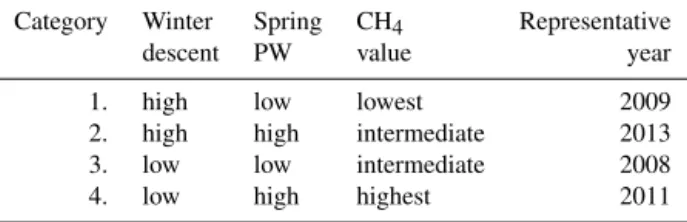
Table 1.Categorization of summer upper stratospheric CH4.
Category Winter Spring CH4 Representative
descent PW value year
1. high low lowest 2009
2. high high intermediate 2013
3. low low intermediate 2008
4. low high highest 2011
PW is planetary wave.
2011 which is the result of the dynamically quiet winter fol-lowed by the FrIAC in early April that caused the CH4to
al-most double. The other 5 years are intermediate, although as noted above, 2010 and 2012 are close to 2009. For all 7 years, once the relative abundances of CH4 were established by 1
May (day 121), they remained mostly unchanged with re-spect to each other until October (around day 280). Figure 2b shows WACCM zonal mean CH4results for 1.47 hPa at the
single latitude of 75◦
N for 2009 and 2008. The reason for sampling WACCM at a single latitude is to test whether the slow seasonal drift of the SOFIE occultation pattern from 65 to 82◦might be affecting our comparisons. While there are
some differences in absolute abundance between WACCM and SOFIE for the first 30–40 days when late winter con-ditions still prevailed, after that, in spring and summer, the agreement between WACCM at one latitude and SOFIE over a small range of latitudes is excellent. Thus we can conclude that the latitude variation of the SOFIE occultations can be neglected. This is not surprising since wave activity and lati-tudinal gradients are relatively weak in summer.
Table 1 presents an idealized categorization of how the summer level of Arctic upper stratospheric CH4 can be
placed in the context of the four categories of wintertime de-scent and early spring dynamical variability. The years 2008, 2009, 2011 and 2013 are most representative of these ideal-ized cases. The other years are more intermediate; as noted above, 2010 and 2012 were closer to 2009 in having rela-tively strong late winter descent of mesospheric air and a relative absence of springtime wave activity (with its asso-ciated horizontal transport of low-latitude air to polar lati-tudes; cf. Siskind et al., 2015a). The year 2014 is closer to 2011. As seen in Fig. 2, there was a 50 % increase in CH4
in late March 2014 and we have previously, tentatively sug-gested that there was a FrIAC event in that spring (Siskind et al., 2015a). Certainly this categorization is qualitative, not quantitative; however, we suggest that it provides a useful framework for analyzing the spring and summer CH4
vari-ability.
3.2 Chlorine monoxide (ClO)
Here we explore the chemical consequences of the CH4
variations illustrated above. CH4 has long been known to
chlo-100 150 200 250 300 Day of year
0.0 0.1 0.2 0.3 0.4 0.5 0.6
Mixing ratio (ppmv)
2011
2010
2008
2009 2012
2013
2014 (a)
SOFIE
(b) WACCM
2008
2009
50 100 150 200 250 300
Day of year 0.0
0.1 0.2 0.3 0.4 0.5 0.6
Figure 2.Comparison of time series of zonal mean CH4mixing ratio at 1.47 hPa.(a)SOFIE data for the indicated years. The data have been grouped into 5-day bins. See Fig. 1 for a discussion of the latitudes.(b)WACCM for 2008 (solid) and 2009 (dashed) at a single fixed latitude of 75◦N.
rine (Solomon and Garcia, 1984). Specifically, the reaction Cl+CH4→HCl+CH3means that active chlorine (ClOx=
Cl +ClO) should vary inversely with CH4. For example,
Siskind et al. (1998) documented an increase in upper strato-spheric ClO during the early years of the Upper Atmostrato-spheric Research Satellite (UARS) mission which was explained as a direct consequence of the decrease in CH4 observed by
Nedoluha et al. (1998). Froidevaux et al. (2000) observed a general anticorrelation between variations in ClO and CH4
at 2 hPa in the tropics. They showed that there should be an inverse relationship between ClO and CH4.
Figure 3 shows that this anticorrelation also exists between high-latitude CH4and ClO at 1.47 hPa during the spring and
summer. It plots monthly averaged SOFIE CH4against MLS
ClO (sampled at the SOFIE occultation latitudes) for the pe-riod May–August. Although there are only seven datapoints for each month (6 in May due to missing data in 2014), the linear correlation coefficients of−0.92 to−0.97 are highly
statistically significant. Note there is a general increase in ClO from late spring to late summer. This is consistent with the seasonal decrease in CH4 and was discussed by
Con-sidine et al. (1998). Concerning the year to year variabil-ity, the highest summertime ClO for the 7-year period is in 2009. This is a legacy of the strong uninterrupted descent which followed the January 2009 SSW. Other years with rel-atively high ClO include 2010 and 2012 which, as we have discussed, were also years similar to 2009 in their combi-nation of winter descent and spring planetary waves. The lowest summertime ClO is in 2011. This is the result of the strong FrIAC event which occurred in April 2011. The gen-eral range of summer ClO which stems from the above win-ter/spring dynamical variability is about 50 %.
Figure 3 also gives the slopes (m) of the linear fit
be-tween ClO and CH4. It shows a tendency for progressively
steeper (more negative) slopes as the summer progresses and methane decreases. In general, all the values of mare
more negative than the value (−0.42 ppbv ppmv−1) quoted
by Nedoluha et al. (2011) for tropical conditions. However,
Nedoluha et al. (2011) make the point that the CH4is
rela-tively high in the tropics (about 0.6 ppmv according to their Fig. 7). Thus the pattern of steeper slopes for lower CH4is
robust across both Nedoluha et al’s and our analyses. This is precisely the pattern one would expect for the inverse power relationships discussed by Froidevaux et al. (2000). Thus the present SOFIE/MLS comparison is consistent with studies using both UARS and ground-based data that showed ClO and CH4 in the upper stratosphere varying with a high
de-gree of anticorrelation.
To get a broader picture of the ClO and CH4changes at
lat-itudes other than the narrow range sampled by SOFIE, Fig. 4 shows the monthly average zonal mean WACCM/NOGAPS ClO and CH4difference fields for August 2009 minus
Au-gust 2008. Profiles that are compared with MLS (for ClO) and SOFIE (for CH4) for the SOFIE occultation latitude
(given by the dashed white line in the color panel) are also shown in the right-hand plots. The comparison between the model and the data is excellent. Since the difference between 2009 and 2008 represents about half the difference between the extreme years discussed above (2009 and 2011), one can multiply the ClO and CH4 difference values in Fig. 4 by a
factor of 2 to get an estimate of the full range. The model shows that the low 2009 CH4and high 2009 ClO shown in
Fig. 4 are part of a broad region of perturbation extending from 40 to 50◦N to the pole and covering the altitude
re-gion between about 1 and 8 hPa. There may be a small verti-cal offset, perhaps one grid point, whereby the model profile is shifted slightly downward relative to both the MLS and SOFIE data. A similar offset was recently noted by (Siskind et al., 2015b) in their WACCM/NOGAPS simulation of the 2009 descent of mesospheric NOx. Since the summer CH4
depletion is a consequence of the winter descent, this off-set may reflect the small discrepancy seen by Siskind et al. (2015b).
Figure 4 shows that the effect of the CH4on ClO occurs
specifi-0.1 0.2 0.3CH4 (ppmv) 0.4 0.5
0.1 0.2 0.3 0.4 0.5 0.6
ClO (ppbv)
r = -0.923
m = -0.61 2008
2009 2010
2011 2012
2013
May Ave lat = 70.5
Pressure = 1.468hPa
0.1 0.2 0.3 0.4 0.5
CH4 (ppmv) 0.1
0.2 0.3 0.4 0.5 0.6
ClO (ppbv)
r = -0.958
m = -.68
June Ave lat = 66.5
2008 2009 2010
2011 2012
2013 2014
0.05 0.10 0.15 0.20CH4 (ppmv) 0.25 0.30 0.35
0.1
0.2
0.3
0.4
0.5
0.6
ClO (ppbv)
r = -0.960 m = -.79
July Ave lat = 68.5
2008 2009 2010
2011 2012
2013 2014
0.05 0.10 0.15 0.20 0.25 0.30 0.35
CH4 (ppmv)
0.1
0.2
0.3
0.4
0.5
0.6
ClO (ppbv)
r = -0.967 m = -1.19
August
Ave lat = 75.8 2008 2009 2010
2011 2012
2013 2014
Figure 3.Scatter plot of zonal mean, monthly averaged MLS ClO vs. SOFIE CH4at 1.47 hPa. The MLS data are sampled at the SOFIE occultation latitude, the monthly averages of which are indicated in each panel. In the upper right of each panel the linear correlation coefficients (r) between each dataset for each month are given, as well as the slope of the linear fit (m) in units of ppbv of ClO per ppmv of CH4.
cally Figs. 2 and 3, represent only the uppermost edge of this larger perturbation. The reason for focusing on this narrower region is that these altitudes, between 1 and 3 hPa, are where the chlorine cycle is affecting the ozone. This is discussed in the next section.
3.3 Ozone (O3)
Figure 5 presents a time series of upper stratospheric ozone from MLS in a format similar to Fig. 2 for CH4. Only 4
years are shown because in summer, the curves almost over-lap and it would be hard to distinguish all 7 years clearly. The 4 years shown correspond to the representative years given in Table 1. The figure shows very large variability in March and April, both intra- and interannually. This is largely driven by the large temperature variability, which itself is dynami-cally driven, as discussed by several authors (Siskind et al., 2015a; McCormack et al., 2006; Smith, 1995; Froidevaux et al., 1989). Of interest here is that after 1 May the interan-nual variability becomes very small, but is not zero. It also shows that the relative abundance from year to year remains generally fixed throughout the summer into the autumn. This small remaining difference is due to chlorine chemistry, as seen below.
Figure 6 shows the zonal and monthly averaged odd oxygen loss rates from the HOx, ClOx and NOx catalytic
cycles for June 2008 and 2009 at 75◦
N calculated by WACCM/NOGAPS. The expressions for these terms are
from Eq. (A1) of McCormack et al. (2006). The figure shows that the contribution to total odd oxygen loss from chlorine chemistry maximizes in a narrow layer from 1 to 3 hPa and that it is greater in 2009 than in 2008. This is consistent with the greater ClO observed by MLS in 2009 as shown in Fig. 3. The HOx cycle shows little change, but the NOx
cycle actually shows the opposite effect, i.e., decreased loss in 2009. This is perhaps surprising and is worth document-ing. Figure 7 shows the monthly averaged NOx (i.e., NO+
NO2) from WACCM for June for 75◦N for 2009 and 2008.
Above the stratosphere, from 1 to 0.1 hPa, NOx was higher
in 2009. This is likely a legacy of enhanced descent from the upper mesosphere observed earlier that spring. However, as discussed by Siskind et al. (2015b) and also by Salmi et al. (2011) in their study of data from the Atmospheric Chem-istry Experiment Fourier Transform Spectrometer, there is no evidence that these enhancements penetrated down to alti-tudes where the NOxcatalytic cycle affects ozone. Although
SOFIE does not measure NO2, the excellent agreement
be-tween WACCM NO and SOFIE NO documented by Siskind et al. (2015b) gives us confidence that the WACCM NOx
re-sults are an accurate reflection of reality. We suggest that the lower NOxfrom 1 to 8 hPa in 2009 is a legacy of greater
win-ter/spring descent from the region of the NO minimum in the mesosphere near 60–75 km.
Thus while there is some offsetting of the changes in the chlorine cycle by the lower 2009 NOx, the net effect is that
30 40 50 60 70 80 90
Delta ClO
-0.02
0.02
0.06
10
1
Pressure (hPa)
10
1
Pressure (hPa)
-0.02 0.00 0.02 0.04 0.06 0.08 0.10 ppbv
10
1
Pressure (hPa)
WACCM
MLS
30 40 50 60 70 80 90
Latitude
Delta CH4
-0.06 -0.02 0.02 0.06
0.10 0.14 0.18
10
1
Pressure (hPa)
10
1
Pressure (hPa)
-0.10 -0.08 -0.06 -0.04 -0.02 0.00 0.02 ppmv
10
1
Pressure (hPa)
WACCM
SOFIE
Figure 4. The color contours on the left are zonal mean WACCM/NOGAPS difference fields for August 2009 minus Au-gust 2008 for ClO (top) and CH4 (bottom). The vertical dashed white line is the mean latitude of the SOFIE occultations for August. On the right, a vertical profile of the model difference at the SOFIE occultation latitude (solid line with plus symbols) is compared with MLS ClO and SOFIE CH4 (data are dotted/dashed curves with stars). Note thatxaxes for the right panels are reversed from one another since the ClO change is positive, while the CH4change is negative.
75
Figure 5. Time series of zonally averaged ozone from MLS at 75◦N.
2009. Between 3 and 7 hPa, it is less in 2009. These changes agree well with observed ozone changes, as seen by MLS. This is shown in Fig. 8 which presents an altitude profile of the ozone change from WACCM/NOGAPS compared with MLS for June at 75◦
N. The figure shows the relative 2009 ozone decrease near 1–2 hPa, corresponding to the increase
0 1•106 2•106 3•106 4•106
Loss rate (cm s )-3 -1
10 1
Pressure (hPa)
NOx cycle ClOx cycle HOx cycle
Figure 6.Altitude profiles of monthly and daily averaged ozone loss rates from WACCM/NOGAPS for June 2009 (solid) and June 2008 (dashed) at 75◦N.
0 5 10 15
ppbv 10.0
1.0 0.1
Pressure (hPa)
Figure 7.Monthly averaged WACCM/NOGAPS NOx (=NO + NO2for June 2009 (solid) and 2008 (dashed) at 75◦N.
in chlorine loss. From 4 to 6 hPa, there is a small ozone in-crease in 2009 which corresponds to the small reduction in NOxloss suggested by Figs. 6 and 7.
Figure 9 shows that the ozone change over the entire 7-year period is consistent with the above analysis for 2008 and 2009. Figure 9 presents monthly averaged correlation coeffi-cients between MLS ozone and MLS ClO (Fig. 8a) and be-tween MLS ozone and SOFIE CH4(Fig. 8b) for 1.47 hPa.
Figure 9a shows that the approximate 5 % spread in ozone values is almost perfectly anticorrelated with the 50 % ClO changes shown in Fig. 3. Further, since we have previously shown that the summer ClO in the upper stratosphere reflects the interannual variability in CH4, it is no surprise that MLS
O3, sampled at SOFIE latitudes, should almost perfectly
cor-relate with SOFIE CH4. This is shown in Fig. 9b.
Finally, Fig. 10 plots the linear correlation coefficient of CH4and O3as a function of altitude. Four curves are shown,
domi--3 -2 -1 0 1 2 3 Percent
10 1
Pressure (hPa)
MLS
WACCM
Figure 8. Percent change in monthly averaged ozone for June 2009 minus June 2008 at 75◦N. The solid line is from
WACCM/NOGAPS and the dashed line with stars is from MLS data.
0.05 0.10 0.15 0.20 0.25 CH4 (ppmv)
3.10 3.15 3.20 3.25 3.30 3.35 3.40
O3
(ppmv)
1.47 hPa Aug
r = 0.960
(b)
2008
2009 2010
2011
2012
2013 2014
0.35 0.40 0.45 0.50 0.55 0.60 ClO (ppbv)
3.10 3.15 3.20 3.25 3.30 3.35 3.40
O3
(ppmv)
2008
2009 2010 2011
2012 2013
2014 1.47 hPa Aug r = -0.95
(a)
Figure 9. Scatter plot of August monthly mean MLS O3 vs. (a)MLS ClO and(b)SOFIE CH4 at 1.47 hPa. The latitudes are near 78◦N, corresponding to the latitude of the SOFIE occultations
in August.
nant and the link to CH4disappears. Thus the effects of
un-interrupted wintertime descent of mesospheric air on ozone may fall into two categories, separated by altitude. From 1 to 2 hPa the ozone reductions result from chlorine enhance-ments; for higher pressures, the potential for NOx
enhance-ments dominates, provided such enhanceenhance-ments were to make it down to those pressures.
0.0 0.2 0.4 0.6 0.8 1.0
r(ch4-o3) 4.0
2.8 2.0 1.4 1.0 0.7
Pressure (hPa)
May Jun
Jul Aug
Figure 10. Altitude profiles of linear correlation coefficients for SOFIE CH4and MLS O3(sampled at the SOFIE occultation lat-itudes). The four curves are taken from zonal mean averages for May (solid), June (long dashes), July (dotted) and August (dot-ted/dashed).
4 Conclusions
We have shown how the chemical composition in the sum-mertime upper stratosphere depends upon dynamical activ-ity from the previous winter and spring. Our main result is to identify a new mechanism for summertime ClO and O3
variability, namely due to CH4variations which, in turn,
pend upon both the magnitude of wintertime mesospheric de-scent and springtime planetary waves. In 2009, prolonged mesospheric descent and a relative absence of springtime wave activity lead to relatively low values of CH4which
per-sisted throughout the summer. At the other extreme, in 2011, the lack of strong winter descent combined with an intense frozen-in anticyclone event in early April led to CH4values
which were more than twice that in 2009.
The excellent anticorrelation between MLS ClO and SOFIE CH4 both validates our understanding of reactive
chlorine partitioning and also offers a framework for inter-preting future observations. Due to orbital precession, the latitudes of the SOFIE occultations have drifted away from polar region and SOFIE is presently unable to monitor win-tertime tracer descent. However, based upon the results in this paper, perhaps MLS ClO data can be used as a proxy for this. It would also be interesting to consider whether these variations in ClO have any impact on O3trend assessments.
Both the strong winter descent and the spring FrIAC phe-nomenon seem to be more common in recent years (Allen et al., 2011; Manney et al., 2005). In principle, the enhanced variability we have shown here might have to be considered, at least for trend studies at high latitudes. Recent estimates of ClO trends (Jones et al., 2011) have only considered the tropics.
Our work shows that these CH4and ClO variations have
gen-eral role of chlorine chemistry in upper stratospheric ozone. This also represents a second mechanism, in addition to that associated with a descent of enhanced mesospheric NOx,
by which descent of mesospheric air can cause ozone re-ductions. Studies of spring- and summertime ozone loss following strong descent years should take care to guish between these two mechanisms. One way to distin-guish them may be according to altitude. Thus ozone de-creases forp <3 hPa (z >40 km) are more likely the result
of low CH4, whereas forp >3 hPa (z <40 km), NOx
en-hancements would dominate. A likely example of this second case is shown in Fig. 1 of Randall et al. (2005).
Finally, the question of whether this variability would in-fluence trend analyses may be worth considering. There was earlier work using Upper Atmospheric Research Satellite data to look at hemispheric differences in ozone trends (Con-sidine et al., 1998); in light of the more recent dynamical variability seen in the NH, and its now documented impact on ozone, perhaps this should be revisited.
5 Data availability
SOFIE data are available on line at http://sofie.gats-inc. com. MLS data are available from the NASA Goddard Earth Science Data Information and Services Center (http: //acdisc.gsfc.nasa.gov). The WACCM model and instruc-tions for its use are available at https://www2.cesm.ucar.edu/ working-groups/wawg.
Acknowledgements. We acknowledge the Aeronomy of Ice in the Mesosphere explorer program from the NASA Small Explorer Program. Two of us (Fabrizio Sassi and Gerald E. Nedoluha) addi-tionally acknowledge funding from the Chief of Naval Research.
Edited by: F. Khosrawi
References
Allen, D. R., Douglass, A. R., Manney, G. L., Strahan, S. E., Kross-chell, J. C., Trueblood, J. V., Nielsen, J. E., Pawson, S., and Zhu, Z.: Modeling the Frozen-In Anticyclone in the 2005 Arc-tic Summer Stratosphere, Atmos. Chem. Phys., 11, 4557–4576, doi:10.5194/acp-11-4557-2011, 2011.
Andrews, D. G., Holton, J. R., and Leovy, C. B.: Middle Atmo-sphere Dynamics, Academic Press, 489 pp., 1987.
Bailey, S. M., Thurairajah, B., Randall, C. E., Holt, L., Siskind, D. E., Harvey, V. L., Venkataramani, K., Hervig, M. E., Rong, P., and Russell III, J. M.: A multi tracer analysis of thermo-sphere to stratothermo-sphere descent triggered by the 2013 Strato-spheric Sudden Warming, Geophys. Res. Lett., 41, 5216–5222, doi:10.1002/2014GL059860, 2014.
Chandran, A., Collins, R. L., Garcia, R. R., Marsh, D. R., Harvey, V. L., Yue, J., and de la Torre, L.: A climatology of elevated stratopause events in the whole atmosphere community climate
model, J. Geophys. Res., 118, 1–13, doi:10.1002/jgrd.50123, 2013.
Considine, D., Dessler, A. E., Jackman, C. H., Roesnfield, J. E., Meade, P. E., Schoeberl, M. R., Roche, A. E., and Waters, J. W.: Interhemispheric asymmetry in the 1 mbar O3 trend: An anal-ysis using an interactive zonal mean model and UARS data, J. Geophys. Res., 103, 1607–1618, 1998.
Eckermann, S. D., Hoppel, K. W., Coy, L., McCormack, J. P., Siskind, D. E., Nielsen, K., Kochenash, A., Stevens, M. H., En-glert, C. R., Singer, W., and Hervig, M.: High altitude data assim-ilation experiments for the Northern Hemisphere summer meso-sphere season of 2007, J. Atmos. Sol.-Terr Phys., 71, 531–551, 2009.
Fiedler, J., Baumgarten, G., Berger, U., Gabriel, A., Latteck, R., and Lubken, F.-J.: On the early onset of the NLC season as observed at Alomar, J. Atmos. Sol.-Terr. Phys., 127, 73–77, doi:10.1016/j.jastp.2014.07.011, 2015.
Froidevaux, L., Allen, M., Berman, S., and Daughton, A.: The mean ozone profile and its temperature sensitivity in the upper strato-sphere and mesostrato-sphere: an analysis of LIMS observations, J. Geophys. Res., 94, 6389–6417, 1989.
Froidevaux, L., Waters, J. W., Read, W. G., Connell, P. S., Kinni-son, D. E., and Russell III, J. M.: Variations in the free chlorine content of the stratosphere (1991-1997): Anthropogenic, vol-canic and methane influences, J. Geophys. Res., 105, 4471–4481, 2000.
Froidevaux, L., Jiang, Y. B., Lambert, A., Livesey, N. J., Read, W. G., Waters, J. W., Browell, E. V., Hair, J. W., Avery, M. A., McGee, T. J., Twigg, L. W., Sumnicht, G. K., Jucks, K. W., Mar-gitan, J. J., Sen, B., Stachnik, R. A., Toon, G. C., Bernath, P. F., Boone, C. D., Walker, K. A., Filipiak, M. J., Harwood, R. S., Fuller, R. A., Manney, G. L., Schwartz, M. J., Daffer, W. H., Drouin, B. J., Cofield, R. E., Cuddy, D. T., Jarnot, R. F., Knosp, B. W., Perun, V. S., Snyder, W. V., Stek, P. C., Thurstans, R. P., and Wagner, P. A.: Validation of Aura Microwave Limb Sounder stratospheric ozone measurements, J. Geophys. Res., 113, D15S20, doi:10.1029/2007JD008771, 2008.
Funke, B., Lopez-Puertas, M., Stiller, G. P., and von Clarmann, T.: Mesospheric and stratospheric NOy produced by energetic particle precipitation during 2002–2012, J. Geophys. Res.„ 119, 4429–4446, 2014.
Garcia, R. R., Marsh, D. R., Kinnison, D. E., Boville, B. A., and Sassi, F.: Simulation of secular trends in the middle atmosphere, J. Geophys. Res., 112, D09301, doi:10.1029/2006JD007485, 2007.
Gordley, L. L., Hervig, M. E., Fish, C., Russell III, J. M., Bailey, S. M., Cook, J., Hansen, S., Shumway, A., Paxton, G., Deaver, L., Marshall, T., Burton, J., Magill, B., Brown, C., Thompson, E., and Kemp, J.: The solar occultation for ice experiment, J. Atmos. Sol.-Terr Phys., 71, 300–315, 2009.
Hess, P.: Variance in trace constituents following the final strato-spheric warming, J. Geophys. Res., 95, 13765–13779, 1990. Hu, J., Ren, R., and Xu, H.: Occurrence of winter stratospheric
sudden warming events and the seasonal timing of spring stratospheric final warming, J. Atmos. Sci, 71, 2139–2334, doi:10.1175/JAS-D-13-0349.1, 2014.
data sets, Atmos. Chem. Phys., 11, 5321–5333, doi:10.5194/acp-11-5321-2011, 2011.
Lahoz, W. A., Geer, A. J., and Orsolini, Y. J.: Northern Hemisphere stratospehre summer from MIPAS observations, Q. J. Roy. Me-teor. Soc., 133,197-211, 2007.
Letexier, H., Solomon, S., and Garcia, R. R.: The role of molecular hydrogen and methane oxidation in the water vapour budget of the stratosphere, Q. J. Roy. Meteor. Soc., 114, 281–295, 1988. Manney, G. L., Kruger, K., Sabutis, J. L., Sena, S. A., and Pawson,
S.: The remarkable 2003-04 winter and other recent warm win-ters in the Arctic stratosphere since the late 1990s, J. Geophys. Res., 110, D04107, doi:10.1029/2004JD005367, 2005.
Manney, G. L., Livesey, N. J., Jimenez, C. J., Pumphrey, H. C., Santee, M. L., MacKenzie, I. A., and Waters, J. W.: EOS Microwave Limb Sounder observations of frozen-in anticy-clonic air in arctic summer, Geophys. Res. Lett., 33, L08610, doi:10.1029/2005GL025418, 2006.
Manney, G. L., Krüger, K., Pawson, S., Minschwaner, K., Schwartz, M. J., Daffer, W. H., Livesey, N. J., Mlynczak, M. G., Rems-berg, E. E., Russell III, J. M., and Waters, J. W.: The evolution of the stratopause during the 2006 major warming: Satellite data and assimilated meteorological analyses, J. Geophys. Res., 113, D11115, doi:10.1029/2007JD009097, 2008a.
Manney, G. L., Daffer, W. H., Strawbridge, K. B., Walker, K. A., Boone, C. D., Bernath, P. F., Kerzenmacher, T., Schwartz, M. J., Strong, K., Sica, R. J., Krüger, K., Pumphrey, H. C., Lambert, A., Santee, M. L., Livesey, N. J., Remsberg, E. E., Mlynczak, M. G., and Russell III, J. R.: The high Arctic in extreme winters: vortex, temperature, and MLS and ACE-FTS trace gas evolution, Atmos. Chem. Phys., 8, 505–522, doi:10.5194/acp-8-505-2008, 2008b. Manney, G. L., Schwartz, M. J., Kruger, K., Santee, M. L.,
Paw-son, S., Lee, J. N., Daffer, W. H., Fuller, R. A., and Livesey, N. J.: Aura Microwave Limb Sounder observations of dy-namics and transport during the record-breaking 2009 Arctic stratospheric major warming, Geophys. Res. Lett., 36, L12815, doi:10.1029/2009GL038586, 2009.
Manney, G. L., Santee, M. L., Rex, M., Livesey, N. J., Pitts, M. C., Veefkind, P., Nash, E. R., Wohltmann, I., Lehmann, R., Froide-vaux, L., Poole, L. R., Schoeberl, M. R., Haffner, D. P., Davies, J., Dorokhov, V., Gernandt, H., Johnson, B., Kivi, R., Kyrö, E., Larsen, N., Levelt, P. F., Makshtas, A., McElroy, C. T., Nakajima, H., Parrondo, M. C., Tarasick, D. W., von der Gathen, P., Walker, K. A., and Zinoviev, N. S.: Unpredecented Arctic ozone loss in 2011, Nature, 478, p. 69, 2011.
Marsh, D. R.: Chemical dynamical coupling in the mesosphere and lower thermosphere, Aeronomy of the Earth’s Atmosphere and Ionosphere (IAGA, Special Sopron Book Series 2), 2011. McCormack, J. P., Eckermann, S. D., Siskind, D. E., and McGee,
T. J.: CHEM2D-OPP: A new linearized gas-phase ozone photo-chemistry parameterization for high-altitude NWP and climate models, Atmos. Chem. Phys., 6, 4943–4972, doi:10.5194/acp-6-4943-2006, 2006.
Nedoluha, G. E., Siskind, D. E., Bacmeister, J. T., and Bevilacqua, R. M.: Changes in upper stratospheric CH4and NO2as measured by HALOE and implications for changes in transport, Geophys. Res. Lett., 25, 987–990, 1998.
Nedoluha, G. E., Connor, B. J., Barrett, J., Mooney, T., Parrish, A., Boyd, I., Wrotny, J. E., Gomez, R. M., Koda, J., Santee, M. L., and Froidevaux, L.: Ground based measurements of ClO from
Mauna Kea and intercomparisons with Aura and UARS MLS, J. Geophys. Res., 116, D02307, doi:10.1029/2010JD014732, 2011. Orsolini, Y. J.: Long lived tracer patterns in the summer polar
strato-sphere, Geophys. Res. Lett., 28, 3855–3858, 2001.
Randall, C. E., Harvey, V. L., Manney, G. L., Orsolini, Y., Co-drescu, M., Sioris, C., Brohede, S., Haley, C. S., Gordley, L. L., and Zawodny, J. M.: Stratospheric effects of energetic parti-cle precipitation in 2003–2004, Geophys. Res. Lett., 32, L05802, doi:10.1029/2004GL022003, 2005
Randall, C. E., Harvey, V. L., Siskind, D. E., France, J., Bernath, P. F., Boone, C. D., and Walker, K. A.: NOxdescent in the Arc-tic middle atmosphere in early 2009, Geophys. Res. Lett., 36, L18811, doi:10.1029/2009GL039706, 2009.
Randall, C. E., Harvey, V. L., Holt, L. A., Marsh, D. R., Kinnison, D., Funke, B., and Bernath, P. F.: Simulation of energetic particle precipitation effects during the 2003–2004 Arctic winter, J. Geo-phys. Res., 120, 5035–5048, doi:10.1002/2015JA021196, 2015. Rong, P., Russell III, J. M., Marshall, B. T., Siskind, D. E., Hervig,
M. E., Gordley, L. L., Bernath, P. F., and Walker, K. A.: Version 1.3 AIM SOFIE measured methane (CH4): Validation and Cli-matology, J. Geophys. Res., submitted, 2016.
Russell III, J. M., Bailey, S. M., Gordley, L. L., Rusch, D. W., Horanyi, M., Hervig, M. E., Thomas, G. E., Randall, C. E., Siskind, D. E., Stevens, M. H., Summers, M. E., Taylor, M. J., Englert, C. R., Espy, P. J., McClintock, W. E., and Merkel, A. W.: Aeronomy of ice in the Mesosphere (AIM): Overview and early science results, J. Atmos. Sol. Terr. Phys. 71, 289–299, doi:10.1016/j.jastp.2008.08.011, 2009.
Salmi, S.-M., Verronen, P. T., Thölix, L., Kyrölä, E., Backman, L., Karpechko, A. Yu., and Seppälä, A.: Mesosphere-to-stratosphere descent of odd nitrogen in February–March 2009 after sudden stratospheric warming, Atmos. Chem. Phys., 11, 4645–4655, doi:10.5194/acp-11-4645-2011, 2011.
Santee, M. L., Lambert, A., Read, W. G., Livesey, N. J., Manney, G. L., Cofield, R. E., Cuddy, D. T., Daffer, W. H., Drouin, B. J., Froidevaux, L., Fuller, R. A., Jarnot, R. F., Knosp, B. W., Perun, V. S., Snyder, W. V., Stek, P. C., Thurstans, R. P., Wagner, P. A., Waters, J. W., Connor, B., Urban, J., Murtagh, D., Ricaud, P., Barret, B., Kleinböhl, A., Kuttippurath, J., Küllmann, H., von Hobe, M., Toon, G. C., and Stachnik, R. A.: Validation of the Aura Microwave Limb Sounder ClO measurements, J. Geophys. Res., 113, D15S22, doi:10.1029/2007JD008762, 2008. Sassi, F., Liu, H.-L., Ma, J., and Garcia, R. R.: The lower
ther-mosphere during the northern winter of 2009: a modeling study using high-altitude data assimilation products in WACCM-X, J. Geophys. Res., 118, 8954–8968, doi:/10.1002/jgrd.50632, 2013. Siskind, D. E., Froidevaux, L., Russell III, J. M., and Lean, J.: Impli-cations of upper stratospheric trace constituent changes observed by HALOE for O3and ClO from 1992 to 1995, Geophys. Res. Lett., 25, 3513–3516, 1998.
Siskind, D. E., Eckermann, S. D., Coy, L., McCormack, J. P., and Randall, C. E.: On recent interannual variability of the Arctic winter mesosphere: Implications for tracer descent, Geophys. Res. Lett., 34, L09806, doi:10.1029/2007GL029293, 2007. Siskind, D. E., Eckermann, S. D., McCormack, J. P., Coy, L.,
Siskind, D. E., Stevens, M. H., Englert, C. R., and Mlynczak, M. G.: Comparison of a photochemical model with observations of mesospheric hydroxyl and ozone, J. Geophys. Res., 118, 195– 207, doi:10.1029/2012JD017971, 2013.
Siskind, D. E., Allen, D. R., Randall, C. E., Harvey, V. L., Hervig, M. E., Lumpe, J., Thurairajah, B., Bailey, S. M., and Russell III, J. M.: Extreme stratospheric springs and their consequences for the onset of polar mesospheric clouds, J. Atmos. Sol.-Terr. Phys., 132, 74–81, doi:10.1016/j.jastp.2015.06.014, 2015a.
Siskind, D. E., Sassi, F., Randall, C. E., Harvey, V. L., Hervig, M. E., and Bailey, S. M.: Is a high altitude meteorological analy-sis necessary to simulate thermosphere-stratosphere coupling?, Geophys. Res. Lett., 42, doi:10.1002/2015GL065838, 2015b. Smith, A. K.: Numerical simulations of global variations of
temper-ature, ozone, and trace species of the stratosphere, J. Geophys. Res., 100, 1253–1269, 1995.
Solomon, S. and Garcia, R. R.: On the distributions of long-lived tracers and chlorine species in the middle atmosphere, J. Geo-phys. Res., 89, 11633–11644, 1984.
Straub, C., Tschanz, B., Hocke, K., Kämpfer, N., and Smith, A. K.: Transport of mesospheric H2O during and after the stratospheric sudden warming of January 2010: observation and simulation, Atmos. Chem. Phys., 12, 5413–5427, doi:10.5194/acp-12-5413-2012, 2012.
Thieblemont, R. N., Orsolini, Y. J., Hauchecorne, A., Drouin, M. A., and Huret, N.: A climatology of frozen-in anticyclones in the spring Arctic stratospehre over the period 1960–2011, J. Geo-phys. Res., 118, D20110, doi:10.1002/2014JD021763, 2013. Waters, J. W.: The Earth Observing System Microwave Limb