APPLICABILITY OF THE EWMA MODEL TO ESTIMATE THE VOLATILITY OF ISTANBUL STOCK EXCHANGE BONDS AND BILLS MARKET

(1)

1. Introduction

Extreme volatilities in financial markets lead to uncertainties with respect to taking forward looking decisions and negatively affect the accuracy of forward looking predictions to a large extent. Especially a particular volatility process referred as “volatility clustering”, in which a succession of large or small scale variations ensue, directly influences the financial market players. Several volatility models are currently used in future projections in financial markets. However, the main question is about which volatility model possesses a stronger predictive power or concerns the sufficiency of the calculated volatility outcomes. In this day and age, financial analysts recognize the significance of volatility prediction methods used in decision making regarding future projections.

In ISE Bills and Bonds Market, primarily Central Bank of Republic of Turkey (CBRT), followed by the exchange members and the banks which were granted permissions from Capital Markets Board (CMB) conduct most of the trading. As the parties participate in the trades, they would like to come up with the right and coherent investment decisions by performing forward looking volatility predictions. From this point of view, the daily and annual volatilities of the TL-denominated interest rates on 6-month and 12-6-month GDS that were traded in ISE Bills and Bonds Market for the period between 12.28.2005 and 12.31.2007 have been calculated in this study from their EWMAs (Exponential

Weighted Moving Averages), which were plotted in accordance with the Nelson-Siegel Model. The reliability level of the calculated volatility values has been back tested, which has demonstrated that the volatilities in financial markets might be successfully estimated by the EWMA model.

2. The volatility concept and development of the Ewma model

Volatility is the statistical measure of the fluctuation in the price of a financial instrument (Butler, 1999: 190). According to another definition, volatility is described as the measure which depicts the magnitude of the price movements in stocks, futures contracts or other financial instruments (Hampton, 2005: 3). In this day and age, volatility estimations carry vital importance for both real sector firms and financial institutions. Volatility is also perceived as the degree of variation that takes place in financial markets in time and analysis of the standard deviation or variance can be

used as the methodology for

measurement of this variation. Besides, as much as volatility is a measure of risk, it is also thought to be reflecting the expectations with respect to the direction of the market. Among the primary models used in volatility projections; historical models, implied models and conditional volatility models such as WEMA and GARCH (Generalized Autoregressive Conditional Heteroskedasticity) could be listed. In this study, explanations and practices based on the EWMA model have been presented.

APPLICABILITY OF THE EWMA MODEL TO ESTIMATE

THE VOLATILITY OF ISTANBUL STOCK EXCHANGE

BONDS AND BILLS MARKET

Prof.

Rıza

ASIKOGLU, PhD

(2)

3. The Ewma model

The EWMA is one of the time-series volatility models that estimate the future volatility by taking the past average volatility into consideration, which are

also widely employed in risk

calculations1. The model has been devised on the assumption that asset

returns are symmetrical and

independently distributed, and proceeds from the presumption of the validity of time-dependant volatility (Bolgün and Akçay, 2005). Exponential weighting is related to how long ago the observations have been made. The weight assigned to an observation t times ago is lambda (λ) times that of the weighting of time t-1

(Akçay, Kayahan and Yürükoğlu, 2009: 77). While the weights of the observations tend to equalize as lambda approaches unity, the weights of latest observations increase as it approaches zero. RiskMetrics2 use the EWMA model to estimate the variance and covariance (volatility and correlation) of multi-variable normal distribution. In the EWMA model, the volatility of the next day explains the volatility of the previous (nth) day. This approach constitutes a better predictive power compared to the traditional methods, which take equally weighted mean variation into account (RiskMetrics, 1996: 81). Taking the exponential moving averages of historical data by assigning the highest weights to most recent observations serves to grasp the dynamic characteristics of volatility and to rapidly reveal small changes. This model incorporates two significant superiorities compared to the equal

1

http://www.pricingtools.eu/sigmamodels/ewma.htm (04.12.2008).

2

Riskmetrics has been founded by JP Morgan in 1994 and conducts research about risk management, corporate governance and financial markets. In 1996, this organization type has become a standard for financial markets and 2 years later, Riskmetrics has become a separate company.

weighting model. First of all, in case of weighting data from the recent past more heavily, the volatility generates a faster response to market shocks. Secondly, following a shock fall in the markets, exponentially weighted mean volatility also drops, because the highest weight is given to the closest data point. The EWMA graph behaves as if it has a memory that fades in time.

EWMA is intensively employed in mostly risk management calculations, pricing of derivatives and estimations of forward-looking forecasts. This model is driven by the values of two principal parameters, time (t) and lambda (λ). The (λ) coefficient used by the model is also named as “constant adjustment” or “decay factor” (smoothing constant) as well (Butler, 1999: 199) and indicates the strength of the related period (time course). The (λ) coefficient takes on a value between 0 and 1 (inclusive) and determines the effective depth of data being used in estimating volatility and the relative weighting that will be applied to the data. The EWMA model performs estimations by incorporating the coefficient of lambda for the most recent returns and a weighted average of the prior projections (Jorion, 2005: 362).

In the model, σn is calculated

from the nth day’s (calculated n-1 days ago) volatility (σn-1) and (un-1) denotes the

last returns in the markets. The return change is calculated in the form of ln(P/Pn-1). As the calculations are

performed, a new (u2) should be calculated and used in variance estimations when a new market observation is made or a fluctuation occurs. Ultimately, the old variance levels or variation of the old market returns will become meaningless. From this point of view, the EWMA model is presented as follows: 2 1 2 1 2

)

1 (

_ 







_n _n

n







u



(1)

(3)

large fluctuation in market variance n-1 days ago, which leads to the expansion of (u2n-1) value. Afterwards, the market

volatility for n days is calculated. As the (λ) coefficient used in the calculations diverges from unity, more recent historical data are weighted more heavily (used for short-term projections). This weighting strategy helps to apprehend the dynamic properties of the input data. Riskmetrics recommends using a general decay factor in volatility calculations for all assets within particular time periods. The recommended adjustment coefficient

is 0.94 for daily data and 0.97 for monthly data. When the same decay factor is used in all calculations, the model simplifies computations involving a sizeable covariance matrix and resolves the problems associated with the scope of volatility estimation (Suganuma, 2000: 4). In the EWMA model, designation of the optimum value for (λ) coefficient is of vital importance since it is the most significant controllable parameter. Coefficients of lambda recommended by RiskMetrics depending on country are displayed in Table 1.

Table 1: The optimum coefficients of lambda by country

Source:Bolgün and Akçay, 2005: 330. Another significant parameter that needs to be determined in the EWMA model along with lambda value is the number of effective observations, because exponential weighing will largely affect the effective number of observations used. In other words, the calculation for each day’s volatility is based on the average volatility for a particular number of days past (such as the previous 100 working days). The primarily required step at this point is to determine of the weighting coefficients that will be assigned to each one of the past 100 days. The weighting (w) formula could be defined as follows:

) 100 ( )

(

90 ,

0

t

t T t

w









 According to this formula, weight of the data belonging to the first day of the past 100 days will be calculated as:

000029513

,

0

90 ,

0

(1001)



Whereas, the volatility estimate of the 2nd day be assigned the following weight:

0.90(100-2) = 0,000032792

The weighting will approach unity towards the last day (0.90(100-100) = 1). As is seen, the forward-looking volatility estimation will be performed in

accordance with the estimated

exponentially weighted average volatility of the past 100 days. For instance, at the

COUNTRIES LAMBDA

ARGENTINA 0.972

INDONESIA 0.992

PHILIPPINES 0.925

SOUTH AFRICA 0.938

SOUTH KOREA 0.956

MALASIA 0.808

MEXICO 0.895

THAILAN 0.967

(4)

lambda value of 0.90, the number of effective days equals 9.99 with respect to weighting a total of 100 days. At a much higher lambda value (0.98), the number of effective observations will rise to 43.37. Hence, the lambda value corresponding to a number of effective observations (Q) could be calculated as given by the equation:







1

veriaralıeı

Q

An approximate decay coefficient (λ) should be selected in volatility and

correlation estimations by using the EWMA model. Besides selecting this coefficient, the number of effective observations whose volatility and correlations will be estimated should also be specified. In Table 2, the coefficients used in EWMA model depending on historical data are exhibited. For example, at a reliability level of 0.99 and (λ) coefficient of 0.98, approximately 228 historical data points should be used to estimate the forward-looking volatility and correlation.

Table 2: The number of effective historical data points used in the EWMA Model

Source: RiskMetrics Technical Document, 1996: 94. Riskmetrics generates its

volatility and correlation estimates from 480 different times-series simulations. This method requires a total of 480 variance and 114,900 covariance estimations. By the virtue of this derived covariance matrix comprising these parameters, the optimal decay factor for each variance and covariance level is chosen. This coefficient values should be periodically optimized by IGARCH5 method. In this study, the optimal decay factors have been reoptimized by using the financial analysis software called Financial Instrument Analyzer (FIA).

3. Generation and application of the data set in Ewma model

(5)

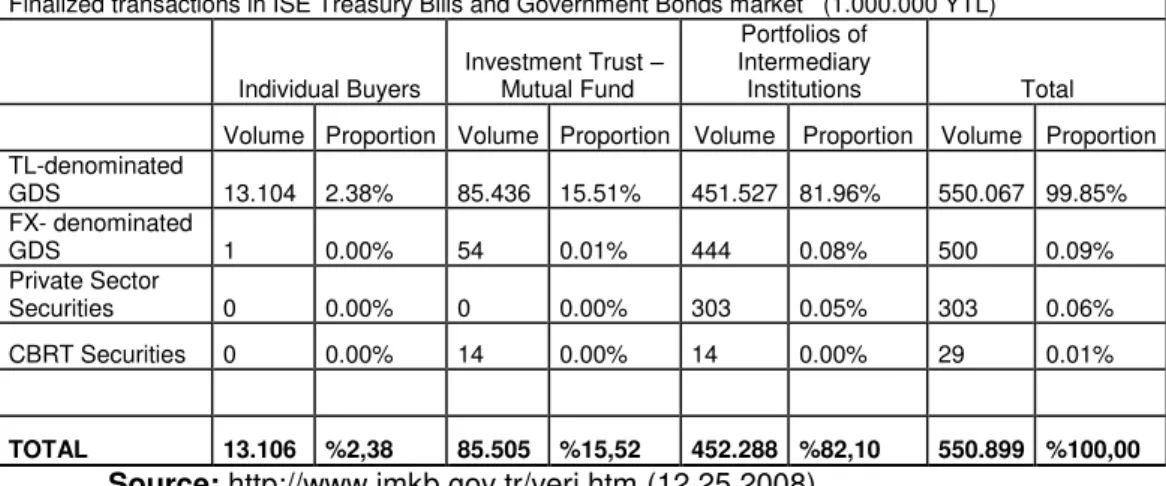
Table 3: Distribution of finalized transactions in ISE Treasury Bills and Government Bonds market for the period between 01.01.2008-11.21.2008

Finalized transactions in ISE Treasury Bills and Government Bonds market *

(1.000.000 YTL)

Individual Buyers

Investment Trust – Mutual Fund

Portfolios of Intermediary

Institutions Total

Volume Proportion Volume Proportion Volume Proportion Volume Proportion TL-denominated

GDS 13.104 2.38% 85.436 15.51% 451.527 81.96% 550.067 99.85% FX- denominated

GDS 1 0.00% 54 0.01% 444 0.08% 500 0.09%

Private Sector

Securities 0 0.00% 0 0.00% 303 0.05% 303 0.06%

CBRT Securities 0 0.00% 14 0.00% 14 0.00% 29 0.01%

TOTAL 13.106 %2,38 85.505 %15,52 452.288 %82,10 550.899 %100,00 Source: http://www.imkb.gov.tr/veri.htm (12.25.2008).

In the study, calculations based on the EWMA model have been deduced from FIA3 (Financial Instrument Analyzer) and the statistical tests were obtained from e-views 5.0. Before proceeding with volatility calculations based on the EWMA model, the yield curve graphs of the GDS interest rates to be used should be plotted with the appropriate model, because considerably different financial instruments with various maturities are traded in the GDS market. Therefore, a disagreement may arise between maturities and interest rates. The correct action here is to estimate the interest rates at the intermediate maturities by assistance of the convenient yield curve model (Teker, Akçay and Akçay, 2008: 5). The Nelson-Siegel model has been used in estimation of the yield curve, because it is the model that produces the projections closest to the actual interest rates observations (Nelson and Siegel,

3

Financial Instrument Analyzer is a financial decision supporting system developed by RiskActive, a financial consulting firm, which can perform calculations pertaining to various fixed or variable income financial instruments and derivates by utilizing internationally accepted financial engineering models and techniques (www.riskactive.com).

(6)

accordance with different methodologies are displayed, with the actual values

additionally presented (Vobjektif, 2004: 25).

Tablo 4. Yield curve analysis for TL-denominated Government Bonds on 12.31.2004

Source:Akçay, 2005: 36.

As seen in Table 4, the Nelson-Siegel model is a yield curve analysis method that provides a close value to the actual observations. Therefore, the interest rates used in this study have been derived by this model. The ultimate goal of the Nelson-Siegel model is to conduct yield estimations of long maturity bonds by projecting them farther in the future than their period of observation (Teker and Gümüşsoy, 2004: 3).

When the data in Table 5 is examined, it is seen that the errors are not normally distributed according to the Jargue-Bera normal distribution test;

since the value of 29.88205 > X20,05 =

5.991. For this reason, logarithmic deviations of foreign exchange rates have been taken as inputs for the conducted analyses. In addition to this, the skewness (S) and kurtosis (K) values show in Table 5 also describe whether the data is normally distributed or not. Accordingly, the magnitude of skewness is 0 and kurtosis is 3 in the case of normal distribution. When these parameters take on fairly different values, the distribution has a skewed or flattened shape and therefore deviates from normality.

Tablo 5. Statistical Results for the GDS

0 10 20 30 40 50 60

14 16 18 20 22 24

Series: INTEREST Sample 12/28/2005 12/31 /2007

Observations 504 Mean 19.19113 Median 19.60900 Maximum 25.33260 Minimum 13.70340 Std. Dev. 2.968496 Skewness -0.365657 Kurtosis 2.057591 Jarque-Bera 29.88205 Probability 0.000000

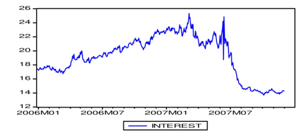
Monthly graph of the time series of the interest rates have been prepared in e-views environment from the data

(7)

Table 6. Evolution of the GDS interest rates between 28.12.2005 – 31.12.2007

12 14 16 18 20 22 24 26

2006M01 2006M07 2007M01 2007M07 INTEREST

For all these reasons, when the stability test of the time series was carried out via ADF (Augmented Dickey-Fuller) test, it was found out that the data did not satisfy the stationary criteria and that the ADF test statistic (0.335277) was below the MacKinnon critical value as seen in Table 7. On the other hand, the

fact that the ADF test result obtained from the first-order differences of the time series (-22.71874) is above the MacKinnon critical value shows that stationary has been maintained in the series. Therefore, the series have become convenient for volatility estimation based on the EWMA model.

Table 7. Stationarity results belonging to the GDS

t-Statistic Prob.*

Augmented Dickey-Fuller test statistic -0.335277 0.9168

Test critical values: 1% level -3.443175

5% level -2.867089

10% level -2.569787

*MacKinnon one-sided p-value

Table 8. Stationarity results for the first-order differences of the time series belonging to the GDS

t-Statistic Prob.*

Augmented Dickey-Fuller test statistic -22.71874 0.0000

Test critical values: 1% level -3.443175

5% level -2.867089

10% level -2.569787

*MacKinnon one-sided p-value

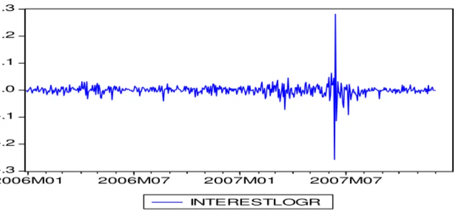
As can been realized from the graph in Table 9 displaying the evolution of interest rate yields, taking the

(8)

Table 9. Evolution of the interest yields on the GDS between 12.28.2005–12.31.2007

-.3 -.2 -.1 .0 .1 .2 .3

2006M01 2006M07 2007M01 2007M07 INTERESTLOGR

It has already been mentioned that the lambda coefficient is the most important parameter that needs to be determined to predict the volatility in accordance with the EWMA model. The lambda coefficients that have been used in this study have been updated by the FIA (Financial Instrument Analyzer) software of RiskActive, because the coefficient of lambda is not constant and varies with time. Thus, it has to be

reoptimized periodically for all financial markets. In this study, the “Lambda Optimizer” feature in FIA has been employed for this purpose. The calculations made as per the algorithm and the obtained optimum lambda figures are displayed in Table 10. Estimations of the 6-month and 12-month volatilities according to the EWMA model are displayed in Tables 11-12 and Tables 13-14, respectively.

Table 10: The calculated lambda coefficients by year

OPTIMUM LAMBDA 2006 2007

6-Month Interest Rate 0.86 0.79

12-Month Interest Rate 0.81 0.93

Source: FIA

Table 11: 6-month volatility estimates as per the EWMA model for year 2006 (λ = 0.86)

(9)

Source: FIA

As seen in the tables, the volatility figures vary with the different lambda coefficients obtained from IGARCH calculations. As the calculations were performed, daily volatilities of the 6-month and 12-6-month GDS had been calculated. Summary of the volatility results for all of the performed estimations are presented in Table 15. In respect of these results, the spread

(10)

Table 15: Summary of the volatility estimation results as per EWMA Year EWMA Estimate ( 6-month) EWMA Estimate (12-month)

2007 (maximum) 0.0419

(10.10.2007)

0.0152 (03.30.2007)

2007 (minimum) 0.0025

(01.09.2007)

0.0052 (13.02.2007)

2007 (mean) 0.009521 0.00928

2006 (maximum) 0.0538

(06.28.2006)

0.1381 (06.28.2006)

2006 (minimum) 0.0025

(04.28.2006)

0.0025 (04.17.2006)

2006 (mean) 0.010821 0.01789

4. Back testing of the ewma estimations

Back testing is the process of testing the validity of the risk model or the volatility figures used by financial institutions in the measurement of the value at risk. It is mainly used for testing the accuracy of risk calculation results and eliminating the model risk. In risk management, the presence of a model risk is tried to be detected through employment of different models. Kuipec (1995) and Crisfersen (1998) are two of the methodologies that most intensively utilize back testing. The fundamental logic in back testing is the comparison of the theoretically estimated and the actually observed values for the following day. Encountering a value outside the range of estimations is recorded as an exception. This operation is performed for each working day. In this way, reliability of the estimations or

calculations is determined.

Overestimating the volatility as a consequence of inaccurate modeling leads to the financial institutions holding more than adequate capital reserves, whereas underestimating the volatility creates mistrust towards the model used by the institution. If the actual volatility is below the calculated volatility, an exception is recorded in the model’s results. If we assume that there are 250 working days in a year, a number of total exceptions between 0 and 13 is considered normal at a confidence interval of 95%, whereas in the case of a higher exception count, the multiplier used in the calculation of capital requirement could be gradually increased for the related financial firm. Other than that, the regulatory institution could demand the review or reconfiguration of the model from the financial institution in cases where the number of deviations exceeds 13 (red area). The distribution of the model with respect to the number of deviations is given below.

Figure 1: Back testing results

Source:Akçay, Kayahan andYürükoğlu, 2009: 26. Deviation number

1 - 2 - 3 - 4

3

5 3+0.4

6 3+0.5

7 3+0.65

8 3+0.75

9 3+0.85

10+

3+1.00

Green area

Yellow area

(11)

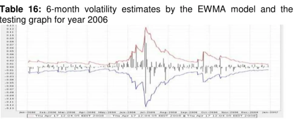
As a result of back testing the values obtained from the tables above, it has been verified at a 99% confidence level that the calculations based on the EWMA model generate successful estimations. Accordingly, the estimated volatilities and back testing graphs for the

6-month and 12-month GDS are

exhibited in Tables 16-17 and Tables

18-19, respectively. Downward or upward deviations can also be traced in these graphs. The summary of results organized from these tables is given in Table 20. As seen in this table, all of the estimates are located in the green area and thereby attest to the acceptability of the model.

Table 16: 6-month volatility estimates by the EWMA model and the back testing graph for year 2006

Source: FIA

(12)

Source: FIA

Table 20: Back testing results

2006 2007

6-month

# of upward deviations # of downward deviations

Lambda (0.86) 2 (0.99) 1 (0.99)

Lambda (0.79) 0 0 12-month

# of upward deviations # of downward deviations

Lambda (0,81) 2 (0.99) 1 (0.99)

Lambda (0,93) 4 (0.98) 1 (0.99) Source: FIA

In parallel to the volatility tests conducted above, the accuracy of the EWMA model and the acceptability of its estimations have been recorded in the risk report published by Banking Regulation and Supervision Agency (BRSA). In this context, the EWMA

model has become the most commonly employed model for estimating the market risks with a usage rate of 84.4%, as shown in Table 21. This figure lends credence to the reliability of the performed estimations and the results of the conducted tests.

Table 21: Usage rates of the volatility estimation models to address market risks (%) Volatility Estimation Model Usage Rate by the Banks

(%)

ARCH 12.5

GARCH 42.8

EWMA 84.4

STOCHASTIC VOLATILITY 3.2

IMPLIED VOLATILITY 18.0

OTHER 12.9

*The sum of the usage rates exceeds 100% since some of the banks employ multiple models

(13)

5. General evaluation and conclusions Today, the financial system is evolving and developing at a rapid pace. The most important factors driving this transformation are time and technology, which lead to the market data display a stochastic distribution rather than a deterministic one. As a consequence, a market structure possessing extremely low kurtosis, volatility clustering and leverage effect makes it much harder to accurately estimate volatilities. In financial markets, various models such as historical and predictive models, EWMA and GARCH can be utilized to estimate volatilities. However, there is not agreement about which one these models constitutes the highest predictive power. Nevertheless, according to 2009

data published by BRSA, the

methodology most commonly employed by the banks is the EWMA model at 84.4%, though it was stated that some banks used multiple models. For instance, while the GARCH method and the implied volatility method is used by 42.8% and 20% of the banking sector, respectively, the usage level for the

ARCH and the Stochastic Volatility

methods are 12.5% and 3.2%,

respectively. The current situation highlights the EWMA model’s superiority compared to other volatility estimation models. In this day and age, accurately estimating the future volatility is essential for financial institutions in the first place and then for businesses operating real economy firms as well. In addition to this, estimation of volatility plays a major part in every field of the financial system from pricing of derivatives to determination of risk management and hedging strategies as well as calculation of portfolio risk.

In this study, 6-month and 12-month volatility estimates with respect to the interest rates in ISE Bonds and Bills Market for the period of 12.28.2005 to 12.31.2007 have been carried out. The performed calculations and the high level of reliability (99%) attained in back testing of the volatility estimates determined as per these calculations have predicated the usability and sufficiency of the EWMA model in analyzing the volatility of interest rates in ISE Bonds and Bills Market.

Akçay Barış (2005) Türev Ürünler ve Uygun Verim Eğrisinin Seçimi, VOBJEKTİF, 6. Sayı,

Eylül 2005, İzmir; AkçayBarış,

Kayahan Cantürk

ve YurükoğluÖzge,

(2009)

Türev Ürünler ve Risk Yönetim Sözlüğü, Scala yayıncılık, İstanbul;

Akinci Özge, Gürcihan Burcu, Gürkaynak Refet ve

ÖZEL Özgür,

(2006)

Devlet İç Borçlanma Senetleri için Getiri Eğrisi Tahmini, TCMB, Araştırma ve Para Politikası Genel Müdürlüğü, No: 06/08. Ankara;

BDDK Bankacılık Sektörü Basel II İlerleme Raporu, Mayıs 2009;

Bolgün Evren ve

Akçay Barış, (2005) Risk Yönetimi, Scala Yayıncılık, İstanbul;

Butler Cormac, (1999)

Matering Value at Risk, Financial Times Prentice Hall, Great Britian;

Giannapoulos Kostas and Eales Brian, (1996)

Futures and Options World, April., http://currencies.thefinancials.com/FAQs1b.html(22.02.2008);

(14)

Hull John C., (2000) Options, Futures, & Other Deriatives, Fourth Edition, Prentice Hall International Inc., U.S.A.;

Jorion Philippe, (2005)

Financial Risk Manager-Handbook, Wiley Finance(Third edition), GARP(Global Association of Risk Professionals), Canada;

Nelson Charles R., Siegel Andrew F., (1987)

Parsimonious Modeling of Yield Curves, The Journal of Business, Volume 60, Issue 4, October, 473-489;

RiscMetrics Technical Document (JP Morgan / Reuters), (1996)

Fourth Editon, 17 December, NewYork;

Suganuma Ricardo, (2000)

Reality Check For Volatility Models, University of California, San Diego Department of Economics, httpwww.econ.puc-rio.brPDFsuganuma.pdf(12.02.2007);

TEKER Suat ve

GÜMÜŞSOY

Levent, (2004)

Faiz Oranı Eğrisi Tahmini: T.C. Hazine Bonosu ve Euro Bond Üzerine Bir Uygulama, 8. Ulusal Finans Sempozyumu, İstanbul.

www.riskactive.com/upload/file/FaizOraniEgrisiTahmn.pdf; Teker Dilek

Leblebici, Akçay Barış ve Akçay Güneş, (2008)

Reel Sektör Kur Riski Yönetiminde Forward ve Opsiyonların Performans Değerlemesi: Ampirik Bir Uygulama, Elektronik Sosyal

Bilimler Dergisi, Cilt 7, S 23, s: 204-222;

Yilmaz Mustafa Kemal, (1999)

İMKB Tahvil ve Bono Piyasasında Gerçekleşen Faiz Oranı Eğrisinin Analizi, Active Finans, Şubat-Mart, İstanbul;