Impacts of climate change scenarios on runoff regimes in the southern Alps

(1)

HESSD

6, 3089–3141, 2009

Climate change and runoffregimes in the

southern Alps

S. Barontini et al.

Title Page

Abstract Introduction

Conclusions References

Tables Figures

◭ ◮

Back Close

Full Screen / Esc

Printer-friendly Version

Interactive Discussion

Hydrol. Earth Syst. Sci. Discuss., 6, 3089–3141, 2009 www.hydrol-earth-syst-sci-discuss.net/6/3089/2009/ © Author(s) 2009. This work is distributed under the Creative Commons Attribution 3.0 License.

Hydrology and Earth System Sciences Discussions

Papers published inHydrology and Earth System Sciences Discussionsare under open-access review for the journalHydrology and Earth System Sciences

Impacts of climate change scenarios on

runo

_ff

regimes in the southern Alps

S. Barontini1, G. Grossi1, N. Kouwen2, S. Maran3, P. Scaroni1, and R. Ranzi1

1

DICATA, Department of Civil Architectural Environmental and Land planning Engineering, University of Brescia, Brescia, Italy

2

Department of Civil and Environmental Engineering, University of Waterloo, Waterloo, Canada

3

CESI RICERCA S.p.A., Milan, Italy

Received: 7 February 2009 – Accepted: 26 March 2009 – Published: 7 April 2009

Correspondence to: S. Barontini (barontin@ing.unibs.it)

(2)

HESSD

6, 3089–3141, 2009

southern Alps

S. Barontini et al.

Title Page

Tables Figures

◭ ◮

Back Close

Full Screen / Esc

Abstract

The potential impact of climate change scenarios on the runoff regime in the Italian Alpine area was investigated. A preliminary analysis of the output of three Global Cir-culation Models (PCM, HADCM, ECHAM) was needed to select IPCC-based scenarios for the 2000–2099 period. Two basins, 1840 and 236 km2in size, respectively, and with

5

different glaciated areas and storage capacity of reservoirs were selected as case stud-ies. The PCM model, the one capable to better reproduce the observed rainfall regime in the investigated area, with the IPCC SRES A2 scenario was adopted for the meteo-rological forcing. On average for the two basins, an increase of annual precipitation of about 3% is expected for the 2050 scenario and should not significantly vary at the end

10

of this century compared to present conditions. At the same time temperature should increase of 1.1◦C in 2050 and 2.4◦C for 2090. Because of the coarse resolution of the climate models’ output, the statistics of the simulated rainy days and daily precipita-tion were adapted to the scale of the two selected basins using a modified version of the multiplicative cascadeβ-model, proposed in the literature to explain the statistics

15

of intermittent fully developed turbulence. As regards to land cover, glaciated areas are decreased, in the future scenarios, according to the Kuhn’s concept of equilibrium line adaptation to climate fluctuations. The tree-line altitude is increased, according to the observed trend since the end of the Little Ice Age: thus boundary conditions for evapotranspiration changed. The resulting meteorological variables and hydrological

20

parameters were used to run the WATFLOOD hydrological model in order to assess the changes of runoffregimes in the two watersheds. A decrease of about 7% of annual runo_ffvolume for the 2050 scenario and of 13% for the 2090 scenario was estimated, on average, at the outlet of the Oglio river basin, the largest one. In the smaller Lys basin, where the glaciated area is 8% of the total area, the annual runoffis foreseen

25

to decrease by about 3% (for the 2050 scenario) and 14% at the end of this century. Also the runoffregime changes are significant, with an increase of spring melt and a decrease of summer and autumn runoff. No clear evidence is found for changes in the

(3)

HESSD

6, 3089–3141, 2009

southern Alps

S. Barontini et al.

Title Page

Tables Figures

◭ ◮

Back Close

Full Screen / Esc

precipitation extremes and in the fraction of rainy days.

1 Introduction

The perception that the Earth is experiencing a fast climate transition, characterised by global warming and changes in the precipitation pattern, is today accepted by most scientists (e.g. Oreskes, 2004; Lovell, 2006), with some exceptions (e.g. Gerhard,

5

2004, 2006). On the basis of experimental evidences, the IPCC 4th Assessment re-port (IPCC, 2007a) and the recent rere-port by Bates et al. (2008) about climate change impact on water resources depict, in summary, the following situation for the Earth’s climate, hydrosphere and criosphere:

– an increase of 0.13◦C per decade is observed for the surface temperature at the

10

global scale over the last 50 years, the double of the last century’s trend, but less than the 0.2◦C per decade observed at the end of the century;

– annual precipitation is increasing in North and South America, northern Europe, northern and central Asia and is decreasing over the Sahel region, the Mediter-anean, southern Africa and part of southern Asia;

15

– Northern Hemisphere snow cover observed by satellite over the 1966 to 2005 pe-riod decreased in every month except November and December, with a stepwise drop of 5% in the annual mean in the late 1980s (IPCC, 2007b);

– glaciers are retreating almost worldwide with a global average annual mass loss of more than half a metre water equivalent during the decade of 1996 to 2005

20

(UNEP-WGMS, 2008), twice the ice loss of the previous decade and over four times the rate of the decade from 1976 to 1985.

(4)

HESSD

6, 3089–3141, 2009

southern Alps

S. Barontini et al.

Title Page

Tables Figures

◭ ◮

Back Close

Full Screen / Esc

Alps, a 90%-significant increase of annual precipitation by 1.6% per decade in the North-Western part and a decrease of 0.5% per decade in the South-Eastern part was observed on the 1950–2000 period. An increase of 0.25◦C vs. an increase of 0.17◦C per decade is observed in the same subregions (Auer et al., 2007).

On the basis of Global Circulation Model’s (GCM) scenarios the IPCC (2007a,b)

5

report confirms, for the future, the observed experimental trends and projects for the current century, at the global scale:

– a global surface air warming ranging from 0.6◦C to 4.0◦C at 2090–2099 relative to 1980–1999;

– globally averaged mean water vapour, evaporation and precipitation are projected

10

to rise with an increase of mean annual precipitation at the global scale ranging from 1.3% to 4.5%, depending on greenhouse gases (GHG) emission scenario over the same period;

– at the end of the 21st century the projected reduction of snow cover in the North-ern Hemisphere ranges between 9% to 17%;

15

– the sensitivity of total glaciers and ice-caps specific mass balance to tempera-ture rise is expected to range from−0.32 to −0.41 m a−1◦C−1corresponding to a specific mass loss ranging from some tens to about 100 m over the century.

At the regional scale, as an example, similar temperature trends were outlined for the Alpine region after an analysis of recent IPCC AR4 scenarios by Faggian and Giorgi

20

(2007), a result confirmed by our study.

More uncertain is the impact on runoff that could have relevant feedbacks, in the near future, on the water management policies (e.g. Parry et al., 1998, 2001) and engi-neering design. No clear signals of runoffchanges at the global scale are documented by the IPCC (Bates et al., 2008), although several studies at the regional scale report

25

about significant variations on a statistical basis in the 20th century. As a balance be-tween precipitation increase and evapotranspiration changes for the current century

(5)

HESSD

6, 3089–3141, 2009

southern Alps

S. Barontini et al.

Title Page

Tables Figures

◭ ◮

Back Close

Full Screen / Esc

Labat et al. (2004) estimate an increase of 4% global amount of runo_ff each 1◦C of temperature increase, even if Legates et al. (2005) do not agree on their conclusions.

Concerning the impact on the hydrological cycle and runoff, the temperature rise will reduce the fraction of precipitation in the form of snow vs. rain. An increase of winter runoff, with respect to the total annual amount, is therefore expected. Snow and ice

5

melt runoffinitiation is expected to anticipate but its total volume depends also on the adaptation to a changed climate of the areal extent of snow and ice fields. Summer melt runoffshould decrease and autumn freezing will start later. With respect to runoff

particularly sensitive will therefore be the regions where snowfall is a significant frac-tion of precipitafrac-tion and melt runo_ff relevant. It is considered a “very robust finding”

10

(Bates et al., 2008) that, in a warming scenario, changes in the runoffregime will be observed particularly in those regions where the ice- and snow-cover are important for the runoffproduction. Many Authors recently pointed out this aspect for various basins characterised by more or less strong glacial- and nival-influence on the runoffregime (e.g. Bobba et al., 1997; Seidel et al., 1998; Pfister et al., 2004; Krysanova et al., 2005;

15

Schaefli et al., 2007).

However the total amount of runoffis also deeply influenced by the evapotranspira-tion losses, which locally depend on a number of factors as the total amount of precipi-tation and its regime, the air temperature and energy exchanges, the climatic feedback on the self-vegetation and anthropogenic effects on the forest cover. The vegetation

20

species in fact can put into action a wide number of different mechanisms in order to react to a climate change (e.g. Walther et al., 2002; Beniston, 2000, for a review). As an example Huntley (1991) focuses on three main kinds of reactions of the vegetation, at the species level, to a climate forcing: genetic adaptation, biological invasion, due to the species competition, and species extinction. Particularly the biological invasion,

25

(6)

HESSD

6, 3089–3141, 2009

southern Alps

S. Barontini et al.

Title Page

Tables Figures

◭ ◮

Back Close

Full Screen / Esc

energy available but also decrease as a negative feedback due to the enhanced stom-atal resistance with the rising atmospheric carbon dioxide concentration. As it was pointed out by Bates et al. (2008), only a few experimental studies are nowadays avail-able in order to formulate a robust hypothesis on the effect of a climate change scenario on the evapotranspiration losses in the water balance.

5

So runoffchanges are likely to be the most uncertain component of the hydrological cycle, especially in mountain areas with transient and seasonal snow cover. There-fore, with the aim of better understanding the e_ffects of climate change scenarios on the runoff regime and water availability in temperate mountain areas, we developed a methodology, based on a hydrological continuous and semi-distributed simulation

10

forced by observations and GCM scenarios for twenty years time windows centred on 2050 and 2090. In our applications we will focus our attention on downscaling of precipitation and temperature and on the feedback of the increase of mean annual temperature on the self-vegetation and glacier’s extent. Our procedure was applied to two meso-scale Alpine basins (1840 and 236 km2 in size) with different glaciated

ar-15

eas and reservoirs’ storage, located in the Po catchment in northern Italy. The runoff

regime of the two basins selected are representatative of those of the Sarca-Chiese-Oglio and Toce-Dora Baltea river systems, respectively, which contribute to about 20% of the national hydropower production. This last was 47.7 TWh a−1 on average in the 2001–2005 period representing about 16% of the national production of energy.

20

In the second section the target areas investigated are described together with the criteria adopted for the selection of the most suitable GCM and projected scenarios. In the third section the downscaling methods to adapt the coarse and biased GCM’s daily precipitation and temperature output to the scale of the two basins are presented. Then the key aspects of the hydrological model and its parameters setup, including the

25

adaptation of vegetation and ice-covered areas to climate change, are summarised. In the fifth section major results of the simulations are presented and discussed.

(7)

HESSD

6, 3089–3141, 2009

southern Alps

S. Barontini et al.

Title Page

Tables Figures

◭ ◮

Back Close

Full Screen / Esc

2 GCM scenarios

2.1 Target areas

Two target areas were selected as case studies: the Oglio river basin at Sarnico (1840 km2), in the central Italian Alps, and the Lys river basin at Guillemore (236 km2), in the northern Italian Alps (Fig. 1). The rationale of this choice is based on the great

5

importance of the hydropower-plants in the two basins, with regard to the national pro-duction, and on the difference of the plant schemes. The Oglio river basin is in fact characterised by a large reservoir capacity, of about 180 hm3 and about 10% of the total basin area is drained by reservoirs. On the other hand, the principal hydropower plant within the Lys catchment located at Pont St. Martin is a run-the-river type, with a

10

negligible storage capacity. The main physiographical data of the two basins are given in Table 1. In the following a brief description of the basins is provided.

In the Oglio river basin, a lefthand tributary of the Po river, the altitude ranges be-tween 187 m a.s.l. at Sarnico at the outlet of Lake Iseo (65 km2) to 3539 m a.s.l. of the Adamello peak. Due to the significant elevation range available for hydropower

15

production, this area has been deeply exploited since the end of the 19th century and the system of dams and interlaced channels built since then is still one of the most important in Italy. The geology is characterised by significant intrusive formations and limestones. The land cover is mainly deciduous and coniferous forest up to the tree-line altitude at about 2000 m. Upstream, the glaciated area accounts for 10.4 km2.

20

The precipitation regime belongs to the so-called alpine sub-litoranean type, as de-fined by Bandini (1931). A sub-litoranean regime, which is typical for some areas in the northern Italy, is characterised by one maximum in spring and one in autumn, with minor di_fferences if it is alpine or appennidic. In the northern part of the basin a tran-sition regime toward the continental type, with only one maximum in the summer, is

25

observed. Glaciers do not significantly affect the runoffregime, which is pluvio-nival. The runo_ffis thus mainly influenced by snow melt in spring and by rainfall in autumn.

(8)

HESSD

6, 3089–3141, 2009

southern Alps

S. Barontini et al.

Title Page

Tables Figures

◭ ◮

Back Close

Full Screen / Esc

river basin, has a total area of 236 km2 at Guillemore, including an interlaced area of 31 km2upstream the Pont St. Martin power plant. The altitude ranges from 894 m a.s.l. at the Guillemore dam to 4532 m a.s.l. of the eastern Lyskamm, a peak of the Monte Rosa massif. The geology is characterised by metamorphic rocks, as micaschist and gneiss in the northern part of the basin, serpentines in the central part and gneiss in

5

the southern. The upper rock layer is massive and pervious only if fractured. It is char-acterised by deciduos and coniferus forest cover up to 1500 m a.s.l., by larch forests up to 2100 m a.s.l. At higher altitudes bare outcropping rocks, adjoint to glaciers and pervious moraines, are the dominant land cover feature. The observed precipitation regime is alpine sub-litoranean and the runoffregime at Guillemore is nivo-glacial with

10

one maximum in late spring (May–June) and a minimum in winter. Within this basin, a sub-basin of 10.4 km2 mainly glaciated is gauged at Lake Gabiet (2380 m a.s.l.). Here another important hydropower plant is located. The runoffregime is of the glacial type, with the main peak in summer (June–July) due to glacier ablation, and a measured total runoffof 1064 mm.

15

2.2 Future climate scenarios

In the Special Report on Emission Scenarios-SRES (IPCC, 2000), based on a reanal-ysis of previous works (see e.g. IPCC, 1994, for a comparison), the Intergovernmental Panel on Climate Change described four possible future storylines (A1, A2, B1, B2), each referring to potential causes of GHG emissions and to their possibile future

dy-20

namics. Forty different scenarios were defined based on the storylines, considering possible demographic, social and economical evolution trends and technological devel-opments as causes for future GHG emissions. Each SRES scenario family assumes one out of the four possible storylines and “do not include additional climate initiatives, which means that no scenarios are included that explicitly assume implementation of

25

the United Nations Framework Convention on Climate Change or emission targets de-fined by the Kyoto Protocol” (e.g. IPCC, 2001) which entered into force only on 16

(9)

HESSD

6, 3089–3141, 2009

southern Alps

S. Barontini et al.

Title Page

Tables Figures

◭ ◮

Back Close

Full Screen / Esc

February 2005. Anyway during the past decade world’s economy has rapidly changed and, also after the recent finantial crisis, it is becoming clear how difficult it is to pre-dict future GHG concentrations resulting from any governmental decision and from the dynamics of the causes of GHG emissions.

However the four storylines and the resulting 40 scenarios still represent a

realis-5

tic ensemble of the future socio-economic context the world will face. We review, in summary:

– A1 scenarios: a future world of very rapid economic growth, global population increasing in mid 21st century and rapid introduction of new and more efficient technologies. Three groups are defined as depending on the energy source which

10

is playing the most important role, with A1FI being fossil intensive, A1T without fossil energy sources, A1B assuming a balance across all sources. As a conse-quence these scenarios cover a wide range of GHG emissions trajectories, thus spanning between pessimistic and optimistic, and can be globally considered as an intermediate family of “weakly pessimistic” scenarios.

15

– A2 scenarios: the future world’s development is very heterogeneous. The popu-lation is always increasing while the technological upgrading is the slowest one, with only little international cooperation. These paradigms should exacerbate the GHG emissions so that A2 scenario is regarded to as a “pessimistic” one. By means of an expression already coined for one of the previous set of scenarios, it

20

is sometimes defined as “Business-as-usual” (Beniston, 2004).

– B1 scenarios: population growth is as for scenarios A1, but the economy is re-ducing the exploitation of the resources and new and more efficient technologies are applied. Accounting for the choice of global solutions for economic, social and environmental sustainability this corresponds to the “most optimistic” family

25

of scenarios.

(10)

HESSD

6, 3089–3141, 2009

southern Alps

S. Barontini et al.

Title Page

Tables Figures

◭ ◮

Back Close

Full Screen / Esc

scenarios A2. The economy grows at an intermediate rate, but less technological adaptation measures are assumed. As the A1 family, B2 scenarios correspond to a “weakly pessimistic” GHG emossions projection.

2.3 Selection of GCM models

For this study three different GCM models (NCEP/NCAR-PCM, MPI-ECHAM4-OPYC3

5

and HADCM3-HADLEY) were initially selected, as a source of the meteorological data, within the World Climate Research Programme’s (WCRP’s) Coupled Model Intercom-parison Project phase 3 (CMIP3) multi-model dataset (see Meehl et al., 2007, for de-tails on the dataset). Selected data were available in the early 2005 at the IPCC Data Distribution Centre. In the following the model will be referred to as PCM, ECHAM and

10

HADCM.

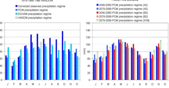
Focusing on precipitation and temperature, for which long time series of observations were available, PCM proved to be more effective than HADCM and ECHAM in repro-ducing the observed monthly regimes of the historical (1979–1999) validation window, as it is shown, as an example, for the Oglio river basin in Fig. 2 (on the lefthand side)

15

and in Table 4. The observed temperature regime is referred to 1398 m a.s.l., the av-erage altitude of the network which is very close to the avav-erage altitude of the basin. The GCM data, instead, are the regimes obtained as an average of the raw monthly data, referred to the height of the local grid cell which is lower, for all the models, be-cause of the smoothed orography adopted. Once the GCM was chosen for the further

20

applications, available daily data were used. The reason why the scenarios were built using only precipitation and temperature series is that only for these variables long time series of observations were available. In order to objectively evaluate the per-formances of the GCMs three different scores were computed for the re-normalised monthly precipitation, as reported in Table 3. These are the root mean squared error

25

of the monthly precipitation regime (M-RMSE), of the cumulative precipitation volumes (V-RMSE) and the maximum absolute error of simulated vs. observed cumulative pre-cipitation volumes (V-MAE). As it can be seen PCM is slightly better than ECHAM in

(11)

HESSD

6, 3089–3141, 2009

southern Alps

S. Barontini et al.

Title Page

Tables Figures

◭ ◮

Back Close

Full Screen / Esc

terms of V-RMSE and V-MAE, and definitively better than HADCM for all the scores. In addition Fig. 2 shows that PCM better captures some patterns of the precipitation regime, as the absolute minimum of precipitation in February and the May-June-July maximum, being the ECHAM monthly distribution too smooth. On the other hand the HADCM-based regime stresses too much the importance of the summer miminum

5

(less than one third of the observed precipitaion in August) vs. the winter one. Such a behaviour would have relevant effects on the hydrological response of the basin.

Then, three different GCM-projected scenarios were selected for two future time windows 2040–2060 and 2079–2099, with the aim of analysing future climate and en-vironmental conditions in a time period centered at 2050 and 2090, respectively. This

10

is close to the idea of checking the e_ffects of potential climate change at the middle and at the end of the current century. With the aim to represent the widest range of possible hydrological responses, scenarios A2, B2 and A1B were firstly selected to build the precipitation and air temperature forcing for the two Alpine basins. As an ex-ample of the inter-model and inter-scenario uncertainty in the precipitation projections,

15

focusing on the Oglio river basin, the total precipitation for A2 scenario ranges from 706.4 mm (HADCM) to 992.2 mm (PCM) at the annual time scale for the 2040–2060 time window, and B2 scenario total precipitation ranges from 734.5 mm (HADCM) to 1059.7 mm (ECHAM).

However, because of the better agreement with observations, PCM-based scenarios

20

were chosen for this analysis. Figure 2 (on the righthand side) and Table 4 show the variability of PCM-based precipitation regimes referring to different scenarios as well as to the two selected future time windows. The annual precipitation is not strongly affected, but the change is more evident at the monthly scale (especially in the fall sea-son) and for the end of the century. Mean annual precipitation for the PCM-A2 scenario

25

(12)

HESSD

6, 3089–3141, 2009

southern Alps

S. Barontini et al.

Title Page

Tables Figures

◭ ◮

Back Close

Full Screen / Esc

for the 2050- and 2090-centered A2-scenario. A strong decrease in the mean annual precipitation is indicated by HADCM-A2 scenario for the same area, of 10% and 24%, respectively, for the 2050- and 2090-centered temporal windows.

The temperature regimes are represented in Table 2. Intermodel differences in mean annual temperature can be in part explained also considering the di_fferent orography

5

adopted by the models which is smoother than the actual one having the grid cell for the Oglio basin in PCM a mean altitude of 800 m, in ECHAM of 850 m and of 500 m in HADCM, thus explaining the 1.8◦C-higher mean annual temperature in comparison with PCM. As GCM grids are very coarse, they cannot reproduce the mountain orog-raphy especially in the Alpine region which is represented by only a few grid points.

10

Therefore, in view of a hydrological application, we corrected the GCM temperature in order that the control scenario reproduces on average the observed historical data. The same bias should therefore apply to the future scenarios. In the A2 scenario, with regard to the nearest grid point to the Oglio river basin, an increase of the mean annual temperature ranging from 1.1◦C (PCM) to 2.7◦C (ECHAM) is projected for 2040–2060

15

with respect to the control simulation, and an increase ranging from 2.4◦C (PCM) to 5.5◦C (ECHAM) is projected for 2079–2099. Lower increases are expected within the framework of the weakly pessimistic B2 scenario, ranging from 1.0◦C (PCM) to 2.6◦C (ECHAM) for 2040–2060, and from 1.7◦C (PCM) to 3.8◦C (ECHAM) projected for 2079– 2099.

20

3 Spatial downscaling of the PCM data

PCM data, but also most of the other GCM-based data as well, are now available at the 1-day temporal scale that can satisfactory meet the requirements of a hydrological simulation aiming at reproducing runoff regimes on a climatological scale, as in our study. Anyway, the linear spatial scale of the grid cell, which is more than 200 km

25

at latitudes of 45◦N, is not suitable for most of the hydrological applications at the mesoscale. The linear scale of the latter can be in fact considered of the order of some

(13)

HESSD

6, 3089–3141, 2009

southern Alps

S. Barontini et al.

Title Page

Tables Figures

◭ ◮

Back Close

Full Screen / Esc

tens of kilometers. Therefore the downscaling of GCM-based meteorological data is a key aspect in the hydrological simulation forced by syntetic data.

Let us first of all focus on the precipitation data. A great number of contributions have been produced for the last two decades focused on the downscaling of GCM-based meteorological data with different approaches (see e.g. Giorgi and Mearns, 1991; Wilby

5

and Wigley, 1997; Prudhomme et al., 2002, for a review). A time-downscaling is nec-essary for the hydrological forcing by GCM data available at monthly or longer time scales (e.g. Burlando and Rosso, 1991; Wilby et al., 2002; Maurer and Hidalgo, 2008) or to project information on extreme runoffevents (e.g. Burlando and Rosso, 2002a,b, for the Arno river basin in central Italy), but it is not needed as the temporal scales

10

of the hydrological and meteorological simulations are similar. Otherwise, even for climatology-oriented hydrological simulations, GCM-based forcing data still require the application of a spatial downscaling procedure through the spatial scales of rainfall fields before they can be used, because of the non-linearity of the runo_ffresponse, the spatial intermittency of the precipitation fields and the hyerarchical structure of rainfall

15

fields (Waymire et al., 1984; Cowpertwait et al., 1996), which cannot be reproduced by GCMs. In fact, the GCM-precipitation being the spatial average on a wide grid cell, local statistics of dry days are not respected and a large number of low intensity rainy events is not able to produce a realistic runoff extimate. Moreover the precipitation fields in mountain regions are a_ffected by regional climatic patterns, orographic e_ffects

20

and local convective phoenomena (as an example, some results on this topic are dis-cussed by Ranzi et al., 1999, and Bacchi and Kottegoda, 1995, for the central Italian Alps). The trough of the annual precipitation measured in the central Po Valley, and its increase in the piedmont areas are examples of the concurrent effect of climatic and orographic patterns (Brunetti et al., 2009). Therefore, taking into account that the best

25

(14)

cor-HESSD

6, 3089–3141, 2009

southern Alps

S. Barontini et al.

Title Page

Tables Figures

◭ ◮

Back Close

Full Screen / Esc

relation structure and (iv) the local inhomogeneities due to orographic effects need to be reproduced in the downscaled GCM field, and the method should be conservative in the sense that (v) the original areal precipitation volume should be preserved. Other statistical properties of the stocastic precipitation process, such as the variance, the frequency distribution and the correlation in time, were verifieda posteriori after the

5

downscaling on an empirical basis.

For the temperature data a simple downscaling was applied instead by correcting the mean daily temperature averaged on the GCM grid cell with an altitudinal bias. Because minimum and maximum daily temperature were required for the hydrological model, the observed min-max ranges at the local and monthly scale were applied to

10

correct the mean daily temperature. Both downscaling procedure are described in detail in the following.

3.1 Precipitation downscaling

In this work a two step downscaling scheme was defined. The first step bridges the gap between the spatial average of the precipitation at the GCM grid scale and at the basin

15

scale. The second one, instead, provides local precipitation patterns for the raingauge stations inside the basin. The patterns are either extracted from a dataset, based on the precipitation events measured in the period 1979–1999, or they are defined by a deterministic orographic correction. The first approach to the pattern extraction was ap-plied to the Oglio River basin. This method accounts for the wide altitudinal range of the

20

catchment area and for the presence of an orographic optimum inside it. The method uses the pattern variability of the precipitation events which can affect the catchment. (An orographic optimum is a range of altitude characterised by a pluviometric maxi-mum, due to moisture condensation driven by an orographic lift of the air masses and convection.) The Lys river basin, the area of which is smaller, was divided in two parts

25

with precipitation following the respective altitude.

Therefore two different datasets, fully described by Ranzi et al. (2005), were used in the downscaling processes. For the first step a regional and coarse dataset of

(15)

HESSD

6, 3089–3141, 2009

southern Alps

S. Barontini et al.

Title Page

Tables Figures

◭ ◮

Back Close

Full Screen / Esc

gauges observations was selected. The gauges are uniformly spread over the Italian Alps and the Po river valley and provide daily rainfall measurements, starting from 1 January 1970, and lasting to 31 December 1994. The central and eastern Alps were chosen as a reference regional scale withℓREG∼252 km determined on the basis of the

minimum rectangular area including all the raingauges. Within this region, two other

5

smaller-scale regions were selected, the central Alps (33 stations,ℓCA∼135 km) and

the Oglio river basin inside the latter (6 stations,ℓ_b∼27 km). The reference regional scale ℓREG is close to the GCM scale ℓGCM∼217 km. A local and denser dataset of

raingauge measurements was then chosen for the second step of the downscaling pro-cedure. It consists of 16 stations in the Oglio river basin and 2 stations in the Lys river

10

basin. Data covers the period from 1 January 1979, to 31 December 2000, and from 1 January 1979, to 31 May 2004, for the stations in the Oglio and the Lys catchment, respectively. The data were then corrected in order to account for the measurement error due to the underestimation of the snowfall by raingauges and the variability of the raingage network density vs. the basin hypsometry, as suggested by Ranzi et al.

15

(1999). A precipitation-correction factor of 1.5 was assumed for the snow fraction of the precipitation, accounting for a linear variation of the snow fraction from 1.0 to 0.0 as the daily mean temperature rises from 0◦C up to 2◦C.

In order to present the downscaling scheme, let us, first of all, defineλ=ℓ1/ℓ2 as a

generic scaling ratio between two characteristic scale lengthsℓ1 andℓ2<ℓ1. The first

20

step consists in a stochastic downscaling of the daily GCM spatial-average precipitation P_ℓGCM

GCM (t) at the GCM grid scaleℓGCM, to a realisation of the daily average precipitation

P_ℓGCM

b (t, x) at a scale ℓb, close to the basin scale. In our notation P

GCM

ℓ_GCM (t), as well

as P_ℓREG

REG (t) with the same symbol but for the oberved data at the regional scale, is

considered a stochastic process with time parametert, and P_ℓGCM(t, x) a stochastic

25

(16)

HESSD

6, 3089–3141, 2009

southern Alps

S. Barontini et al.

Title Page

Tables Figures

◭ ◮

Back Close

Full Screen / Esc

The realisationP_ℓGCM(t, x) should first of all be consistent with the observed annual precipitation over the spatial domain at all the ℓ-scales of the hystorical data. This property is considered to be achieved if the time-average E [P_ℓ(t, x)] of the observed precipitation P_ℓ(t, x) at the scale ℓ, is the same of the respective downscaled GCM process, i.e.

5

E [Pℓ(t, x)]=E h

P_ℓGCM(t, x)i. (1)

A realisation for P_ℓGCM(t, x), with the above properties, can be obtained with the following downscaling:

P_ℓGCM(t, x)=α_cα_r(x)α_p(t, x)PGCM(t). (2)

The coefficients introduced in Eq. (2) have the following meaning:

10

– αc is a deterministic climatic coefficient accounting for a bias in the annual mean

of the GCM control simulation vs. the experimental data at the regional scale ℓREG. Defining the spatial average at the regional scale P

REG

ℓ_REG (t)=hP(t, x)iℓ_REG

thenα_cis defined by:

α_c =

EhP_ℓREG

REG (t) i

EhP_ℓGCM

GCM (t)

i; (3)

15

– αr(x) is a deterministic spatial orographic weight accounting for the bias of the

mean observed precipitation EhPℓb(t, x) i

, at the basin scaleℓb, with respect to

the mean observed precipitation EhP_ℓREG

REG (t) i

at the regional ℓREG-scale. It is

therefore given by:

αr(x)=

EhP_ℓ_b(t, x)i

EhP_ℓREG

REG (t)

i, (4)

20

(17)

HESSD

6, 3089–3141, 2009

southern Alps

S. Barontini et al.

Title Page

Tables Figures

◭ ◮

Back Close

Full Screen / Esc

and, by the linearity of expectations, one has:

hαr(x)iℓ_REG =1; (5)

– αp(x, t) is a stochastic multiplicative coefficient, accounting for the probability that

a rainy day at a larger scale is still rainy at a subscale. The stochastic process αp(x, t) is assumed to be homogeneous in space and time. To define αp(x, t) 5

we will apply the concepts inherent in theβ-model originally proposed by Novikov and Stewart (1964) and later developed by Frisch et al. (1978) and Benzi et al. (1984) to explain some statistics of intermittent fully developed turbulence. Our choice was justified because of the simplicity of the model and because we were interested mainly in the representation of rainfall and runoff regimes rather than

10

on the extremes. One starts from a field characterised by a scale lengthℓ1 and

unitary average energy over the whole area. The hypothesis that in the field at a smaller scale the energy splits in active and inactive cells, i.e. without energy, was introduced. The model then suggests possible realisations of the downscaled field of energy, with scaling lengthℓ<ℓ1, in order to preserve the total energy of

15

the upper scale field. With a conceptual similarity with the downscaling of en-ergy in turbulence, considering that the spatial pattern of precipitation is largely influenced by the turbulent structure of the atmosphere and by the dissipation of energy in localised convective cells, such mono-fractal and, later, multi-fractal models (e.g. Lovejoy and Schertzer, 1990; Gupta and Waymire, 1993; Deidda,

20

2000) have been used in order to describe and reconstruct the properties of pre-cipitation fields at different scales as well. The precipitation should then be sub-stituted to the energy in the model and active cells are those where it is raining, while inactive cells represent dry areas.

The multiplicative coefficientsα_p(t, x) concentrate the spatial average

precipita-25

tion P_ℓ

1(t, x), given at the reference scale, in wet areas with higher precipitation

(18)

HESSD

6, 3089–3141, 2009

southern Alps

S. Barontini et al.

Title Page

Tables Figures

◭ ◮

Back Close

Full Screen / Esc

Let us define β the “persistency” of the precipitation process across two spatial scales, i.e. the probability that at a given time a sub-cell at the scaleℓ2<ℓ1is still

rainy when precipitation occurs at the larger scaleℓ1. By generating independent

and identically distributed random values b with a uniform distribution in [0,1], then the random weights αp will have a binomial distribution with the following 5

values:

αp(x, t)=

0 ifb > β=λ−c

λc ifb≤β=λ−c . (6)

In Eq (6) c>0 is the mono-fractal codimension of the precipitation field, being c=2−D, with D the mono-fractal dimension of the 2-dimensional field. The pro-cedure to estimate the parameter of Eq. (6) will be explained in Sect. 3.1.1. Here

10

it is only recalled that, by construction,αp(x, t) is a homogeneous and stationary

stochastic process with unit mean:

hα_p(x, t)iℓ =1, (7)

E

α_p(x, t)

=1. (8)

In order to apply it to downscale the GCM-simulated precipitation to the ℓ-scale

15

of interest, a scaling ratio

λ= ℓ

∗

GCM

ℓ (9)

should be applied. In Eq. (9)ℓ_GCM∗ is an equivalent virtual GCM scale, for which the statistics of dry days are coherent with those of the experimental data at a regional scale. In our work we found, for PCM precipitation data,ℓ_GCM∗ =1737.3 km

20

(for further details, see Sect. 3.1.1).

(19)

HESSD

6, 3089–3141, 2009

southern Alps

S. Barontini et al.

Title Page

Tables Figures

◭ ◮

Back Close

Full Screen / Esc

Taking the expectation of the downscaled precipitation expressed by Eq. (2), by means of the definitions (3, 4, 6) and of the relationships (5, 7, 8), and accounting for the statistical independency ofPGCMand αp, one can verify that the mean annual

precipitation is conserved throughout all the averaging scalesℓ. The procedure de-scribed up to now allows to downscale historical GCM data down to the ℓ-scale of

5

interest. It is applied also to future GCM scenarios assuming stationarity in time of the α_pprocess.

In Figure 3 the cumulative frequency of exeedance is represented for the spatial average at the basin scale of the measured and for the PCM-simulated daily precipi-tation. As discussed above, it is shown that the original PCM dataset is characterised

10

by higher probability of rainy days than the observed ones, and lower cumulative fre-quency of exeedance at higher values of daily precipitation. Moreover it can be ob-served that for the plotted grid-point, which corresponds to the nearest one to the Oglio river basin area, no significant change of the statistics of daily precipitation, neither in the dry days nor in the extremes, is projected for the future scenarios. Otherwise both

15

the downscaled PCM-simulated series for the historical period and the PCM-projected series for the future scenarios are in good agreement with the fraction of dry days, cor-responding to the atom in the origin of the probability distribution, and the cumulative frequency of exeedance of the measured data. As a further a posteriori verification of the effectiveness of the multiplicative cascade model, the variance of the downscaled

20

GCM data for the control period was 49.5 mm2vs. 47.4 mm2of the observed data. A further step of the disaggregation scheme consists in an analogue downscaling of the spatial average of the daily precipitation P_ℓGCM(t, x) to the daily precipitation at the i-th raingauge station P_iGCM(t, x_i). Focusing on the basin-centered, coarser, historical dataset, for eachk-th rainy day the precipitation pattern is defined by way of

25

the normalised precipitation at eachi-th raingauge station (pk,i), i.e.:

p_k,i = Pk,i

(20)

HESSD

6, 3089–3141, 2009

southern Alps

S. Barontini et al.

Title Page

Tables Figures

◭ ◮

Back Close

Full Screen / Esc

in whichP_k,i is the daily precipitation measured at thei-th raingauge station and P_k,ℓ is, as before, the spatial average precipitation at the basin scale ℓ. By applying the classical Thyssen-Voronoi scheme to determine the average spatial precipitation in a basin, one has, by definition:

Pk,ℓ = X

i

wiPk,i, (11)

5

wherew_i are the Thyssen-Voronoi weights of each raingauge. Accounting for Eq. (10), one therefore obtains:

X

i

wipk,i =1. (12)

Equation (12) verifies that the superimposition of a pattern set (pk,i), based on the

his-toricalk-th rainy day, on the average spatial precipitation P_jGCM, will preserve both the

10

spatial average and the spatial correlation structure of precipitation. This completes the downscaling process of the precipitation. Measured and PCM-simulated precipita-tion regimes, both original and downscaled, are represented in Table 4, jointly with the simulated runoff.

3.1.1 The stochastic processαpfor downscaling the precipitation data 15

It was observed that the fraction of wet days nw=Nw

N_tot, being Nw the number of days

with positive precipitation over the total number of daysNtot, if averaged at theℓ-scale,

increases with the length scale with a power law as shown in Fig. 4:

nw,ℓ₁ =nw,ℓ₂λc, (13)

beingλthe scaling ratio

20

λ=ℓ1

ℓ2

. (14)

(21)

HESSD

6, 3089–3141, 2009

southern Alps

S. Barontini et al.

Title Page

Tables Figures

◭ ◮

Back Close

Full Screen / Esc

From the slopecof this power law on a logarithmic chart the mono-fractal codimension of the precipitation field was estimated as c=0.195. Because of our hypothesis of stationarity and homogeneity, statistics of rainy areas can be derived from the time series of precipitation averaged at different scales centered on the target basin.

As a consequence of Eq. (6), in view of mass conservationPℓ₁, each rainy cell at the 5

ℓ2-scale will receive a precipitation intensity Pℓ2 given by the enhancement by a factor

λc of the upper scale precipitation intensityP_ℓ₁:

P_ℓ

2 =Pℓ1λ

c_. ₍₁₅₎

It was observed that the estimated probability of wet days for GCM simulation of the control period, n_w,ℓ_GCM, was significantly higher than the corresponding observations

10

at the same scale. Therefore, having already estimated the value of c, by means of Eq. (13) it was possible to determine the virtual GCM scale ℓ_GCM∗ , we introduced before, and characterised by a probability of wet days in agreement with the historical data. The corresponding point is represented by a red dot in Fig. 4.

3.2 Temperature downscaling

15

In order to downscale the mean daily (j-th) temperature given at the reference GCM cell, T_jGCM, the experimental annual climatic mean Ty, at the basin scale, was

con-sidered as a reference value to be achieved in the historical scenario. Moreover the experimental deviation of the monthly (m-th) mean at each station,Ti ,m=E[T_{i ,j}]_m, from the monthly mean at the basin scaleTm=hTi ,miwas intended to be respected. These 20

results were achieved by defining the mean daily corrected temperatureT_{i ,j}GCM, at the i-th station and after GCM data in the control run, by means of the following two steps corrections of the GCM daily temperatureT_jGCM:

(22)

HESSD

6, 3089–3141, 2009

southern Alps

S. Barontini et al.

Title Page

Tables Figures

◭ ◮

Back Close

Full Screen / Esc

The first bias applied, δT_{i ,m}, is a monthly shift accounting for the difference between Ti ,m and the monthly mean of all the stations in the river basin,Tm, and it is therefore

defined by:

δT_{i ,m} =T_{i ,m}−T_m. (17)

The second one is a yearly shift, accounting for a modeling bias, i.e. the di_fference

be-5

tween the climatic mean of all the meteorological stationsTy=hE[Ti ,j]yiand the climatic

mean of the GCM-dataTyGCM=E[TjGCM]y:

δT_yGCM=Ty−TyGCM. (18)

By averaging on the annual scale the GCM-control run temperature at a stationi and by means of Eqs. (17,18), one obtains that:

10

T_{i ,y}GCM=Ti ,y. (19)

This means that the mean annual value of the simulated temperature is the same as the observed one for each station. As a consequence, also at the basin scale, the annual mean temperature after GCM-data correction is the same as the experimental one:

15

T_yGCM=hT_{i ,y}GCMi=T_y. (20)

The monthly deviationδT_{i ,m}GCMfor the downscaled data, defined as

δT_{i ,m}GCM=E[T_{i ,j}GCM]_m− hE[T_{i ,j}GCM]_mi, (21)

can also be determined from Eq. (16) by applying the expected value operator E[·]m

and then the spatial averaging operatorh·i, keeping into account of Eqs. (17,18). One

20

gets:

δT_{i ,m}GCM=Ti ,m−Tm =δTi ,m, (22)

(23)

HESSD

6, 3089–3141, 2009

southern Alps

S. Barontini et al.

Title Page

Tables Figures

◭ ◮

Back Close

Full Screen / Esc

i.e., the mean experimental monthly deviation is respected for the downscaled data. Finally, being the spatial averaged monthly temperature of the corrected GCM:

hE[T_{i ,j}GCM]_mi=T_mGCM+δT_yGCM, (23)

accounting for Eq. (18), one gets:

hE[T_{i ,j}GCM]_mi −Ty =TmGCM−TyGCM. (24)

5

The latter means that the annual regime of the GCM temperature series is maintained, on average, at the basin scale. Measured and PCM-simulated temperature regimes are represented in Table 2.

4 Hydrological simulations

4.1 Simulation hypotheses

10

At the hydrological mesoscale the atmospherical system and the hydrological system can be considered uncoupled as the hydrological feedback on the atmospherical pro-cesses has already been taken into account in the GCM through approximate schemes. Moreover, the amplitude of the time windows chosen for the simulation of the hydro-logical response to the climate forcing, which are significant from a water resources

15

management point of view, are quite short as compared to the time scales of the cli-mate change. In this study simulations were therefore driven by the concept that the hydrological system could be considered a steady dynamical system during a time window of 20 years, i.e. during the time window of the simulation the effects of the tem-perature and precipitation trends were assumed to be negligible against those due to

20

(24)

HESSD

6, 3089–3141, 2009

southern Alps

S. Barontini et al.

Title Page

Tables Figures

◭ ◮

Back Close

Full Screen / Esc

4.2 Expected response in mid-latitude natural systems to a climate change sce-nario

Data reported in Sect. 2.3 point out that the trend of the mean annual temperature will probably be more important than the variation in the annual precipitation amount in characterising the effect of climate change scenarios on the hydrological cycle of the

in-5

vestigated basins. As many Authors suggest, an increase of even a few degrees in the mean annual temperature can have significant feedbacks on the mid-latitude natural systems. Relevant effects were in fact observed on the evolution of the self-vegetation (Theurillat and Guisan, 2001; Walther et al., 2002; Pelfini et al., 2004; Caccianiga et al., 2008) and on the snowpack and glacier equilibrium-line altitude (Kuhn, 1981;

Braith-10

waite, 2008). In this work two main natural-systems’ feedbacks were taken into account in order to draw future scenarios for the basin land cover: (i) the rise of the tree-line altitude and (ii) a reduction of the glaciated area.

It is a common feeling that a slight climate warming is often accompanied by the rise of the tree-line at the expenses of pasture and grass at the highest altitudes. This

pro-15

cess can be accelerated, in the investigated regions, by afforestation and reforestation processes due to the decline of the wood use for fuel and to the abandonment of the high-altitude pastures (FAO, 2007). In the Mella river basin, a lefthand tributary of the Oglio river in its lower course, Ranzi et al. (2002) observed a significant afforestation and reforestation process in the mountains, jointly with an increase of the urbanised

20

area in the valley. In view of a long-time hydrological simulation, it is important to stress the hydrologically different behaviour of grass- and forest-covered land with regards to the basin evapotranspiration losses. Therefore, according to Galloway (1988), a rise of the tree-line of 100 m altitude was assumed, on average, every 1◦C of mean annual temperature. By a cross comparison of CORINE land cover maps and a digital

eleva-25

tion model of the investigated areas, bare soil and grass-covered soil were reclassed as forest for a belt from 200 to 250 m, over the actual tree-line, for the 2079–2099 scenario.

(25)

HESSD

6, 3089–3141, 2009

southern Alps

S. Barontini et al.

Title Page

Tables Figures

◭ ◮

Back Close

Full Screen / Esc

The rise of the glacier line of equilibrium, and the consequent reduction of the glaciated area, was estimated for the Lys river basin, where the glacier significantly affects the hydrology of the basin. The adopted criterium is based on an energy bal-ance at the equilibrium line of the glacier and it is an application of the concept origi-nally proposed by Kuhn (1980, 1981). The application is based on the hypothesis that

5

the cumulative accumulation C equals the cumulative ablation and allows the deter-mination of the rise of the equilibrium line∆h. Following Ambach and Kuhn (1985), assuming the variation of the site cloudiness negligible, the variation of the sensible flux ∆H_s and of the net radiation ∆R can be parametrised with respect to the mean annual temperatureT_y

10

∆Hs=α∆Ty (25)

∆R =α′∆T_y, (26)

and the equilibrium line rise _∆h, relative to the future-scenario projected variation of the mean annual temperature∆T_y, can be expressed by the relationship:

∆h

∆Ty =

α′+α

L

τ∂C∂z −(α′+α) ∂Ty

∂z

. (27)

15

The numerical values used in Eq. (27) are given: L=0.334 MJ kg−1, latent heat of fusion, τ=60 d, duration of the ablation period, α′+α=1.66 MJ◦C−1m−2d−1, ∂C/∂z=1 kg m−2m−1(accumulation gradient) and∂T_y/∂z=−0.0065◦C m−1 (tempera-ture gradient). The Kuhn’s concept applies to a comparison of equilibrium states. Then, in order to account for the actual disequilibrium of the glaciers, the rise∆hwas applied

20

(26)

HESSD

6, 3089–3141, 2009

southern Alps

S. Barontini et al.

Title Page

Tables Figures

◭ ◮

Back Close

Full Screen / Esc

4.3 Hydrological model

The distributed flood-forecasting model called WATFLOOD (http://www.watflood.ca) Version 9.2.37, compiled on 20 April 2006, was used for our simulations. WATFLOOD is based on the concept of the Group Response Unit (GRU): all hydrologically similar areas within a hydrological model grid are grouped in one unit, then each area

be-5

longing to the same unit receives equal meteorological forcing and the group of areas is treated as one modelling unit, no matter the distance among single areas (Kouwen et al., 1993). The structure of the code is suitable for basin time responses ranging from one hour to several weeks.

The model takes into account all the main hydrologic processes: interception,

infil-10

tration, evapotranspiration, interflow, baseflow, overland routing and channel routing. The Philip formula (Philip, 1954) is used to estimate the infiltration losses. Overland flow and channel routing are done by a storage routing scheme with time steps chosen to satisfy the Courant criteria everywhere. WATFLOOD was previously applied to the Columbia River in the Rocky Mountains in Canada (Kouwen et al., 2005) and, for the

15

European Alps, to the Toce area (Grossi and Kouwen, 2004) and to the Danube area (Benoit et al., 2004).

For this study an important role is played by the evaluation of the intensity of the evapotranspiration process because changes in the total runoffare basically given by those of the precipitation and evapotranspiration losses. As it is widely accepted that

20

an increase in the mean annual temperature could increase the potential evapotranspi-ration, and some experimental measurements seem to confirm this effect showing an increase of the observed evapotraspiration (e.g. Genovese et al., 2005; Rosenzweig et al., 2008 and, for the Italian region, Moonen et al., 2002), otherwise some Authors pointed out that an increase in the carbon dioxide concentration in the atmosphere

25

could increase the stomatal resistance to the evapotranspiration, thus reducing the evapotranspiration losses (Gedney et al., 2006) and leading to an increase of the total runoff(Betts et al., 2007). In this work, accounting for a change in the self-vegetation

(27)

HESSD

6, 3089–3141, 2009

southern Alps

S. Barontini et al.

Title Page

Tables Figures

◭ ◮

Back Close

Full Screen / Esc

equilibrium and in a consequent species redistribution which is intended to optimize the transpirative capabilities of the plants, we adopted a theoretical framework based on the use of the temperature data to estimate the potential evapotranspiration (PET). In the following a full description of the coding scheme referring to the potential and to the actual evapotranspiration is reported.

5

PET was evaluated through the Hargreaves equation which can be used when only temperature data are available. The Hargreaves model is empirical in nature and with some recent modifications (Hargreaves and Samani, 1982) takes the form:

PET=0.0075R_aC_tδ_t1/2Tavg,d (28)

where PET is the potential evapotranspiration rate (mm d−1), Ra is the total incom-10

ing extraterrestrial solar radiation in the same units as evaporation (mm d−1), C_t is a temperature reduction coefficient which is a function of relative humidity (−), δt is

the difference between the mean monthly maximum and mean monthly minimum tem-peratures (◦F), and Tavg,d is the mean temperature (◦F) in the time step. With some

empirical relationships it is possibile to estimate incoming solar energy as a function of

15

air temperature, latitude and julian day.

Up to three coefficients have been applied to reduce the calculated PET to the actual evapotranspiration. The first coefficient, the Upper Zone Storage Indicator (UZSI), es-timates the evapotranspiration as a function of the soil moisture in the upper soil layer (UZS). Evapotranspiration is assumed to occur at the potential rate if the soil

mois-20

ture is at a level of saturation (SAT) and is reduced for soil moisture values below the saturation down to zero at the permanent wilting point (PWP) according to equation:

UZSI= s

UZS−PWP

SAT−PWP (29)

The root of the fraction is used to simulate the increased difficulty with which moisture is extracted by vegetation as the soil dries. The second reduction coefficient (FPET2)

ap-25

(28)

HESSD

6, 3089–3141, 2009

southern Alps

S. Barontini et al.

Title Page

Tables Figures

◭ ◮

Back Close

Full Screen / Esc

which is accumulated beginning on 1 January. The third coefficient used to reduce the PET is a function of the vegetation type. For tall vegetation, it has been shown that the evapotranspiration is significantly less than the potential rate (Spittlehouse and Black, 1981; Price, 1987). Typical values of AET from tall vegetation range from 60 (Stagnitti et al., 1989) to 90% of the PET. Past simulations have successfully used a reduction

5

coefficient of 0.70 applied to the PET rate for the coniferous land classification.

The final reduction in transpiration is a function of the interception. Evaporation of intercepted water is assumed to occur preferentially to soil water transpiration. The sum of the atmospheric resistance and stomatal resistance to water evaporating from stomatal cavities is assumed to be greater than the atmospheric resistance to water

10

evaporating from the surface of the vegetation. In each time step, the transpiration is reduced to zero during periods when interception evaporation (IET) is occurring.

Hydrological and geomorphological characteristics of the two basins were derived from a 1 km resolution DEM. The maps provided the land use, glacier extension and the surface soil conductivity at saturation.

15

5 Results and discussion

5.1 Results

For both the investigated basins, a calibration of the hydrological model was first per-formed on the basis of the measured data (years 1979–1999). Important pieces of information concerning hydropower management are the mean annual runoffvolume,

20

the runoff regimes and the low flow components of the hydrograph. Therefore, by choosing a shorter time window of two years, the calibration focused on the infiltration, storage, evapotranspiration and percolation processes, in order to properly reproduce, at the daily scale, the slow components of the runoffand the baseflow. Key properties were considered the upper soil hydraulic conductivity at saturation, the soil-water

reten-25

tion and the lower zone recession functions. A two-years window (1979–1981), chosen

(29)

HESSD

6, 3089–3141, 2009

southern Alps

S. Barontini et al.

Title Page

Tables Figures

◭ ◮

Back Close

Full Screen / Esc

in order to realistically assume the initial conditions of no snow covering the ground for the two basins, was used for the calibration of the model. Then the long time window 1979–1999 was simulated at the daily scale for a finer tuning of the parameters. As an example, on the basis of the available information and of our field and laboratory ex-periments in nearby Alpine catchments (Barontini et al., 2005, 2009), an average

con-5

ductivity value of about 0.2 mm h−1was appropriate for the Lys catchment and slightly lower values were adopted for the Oglio river basin. Such low values account for shal-low, non mature soils with a compact underlying bedrock, thus producing a Hortonian runoffeven for low rainfall intensity. A snow-melting factor of 0.2 mm◦C−1h−1 for both basins reasonably represented the observed runoffduring the melting period.

10

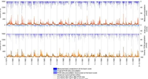
In Fig. 5 the results of the control period simulations are represented for the Oglio river basin at Sarnico and compared with the measured data. Similar results were obtained for the Lys river basin. Observed daily runoffat Sarnico, at the outlet of Lake Iseo, were defined by means of the continuity equation, knowing the outflows of the lake and its stage level. Both the calibration simulation with measured data (upper

15

part of the Figure) and the historical simulation driven by PCM-based downscaled data (lower part) are represented. In the central part of the Figure the original PCM-based precipitation data is shown. Low flows in winter are captured by the hydrological model. The 50% underestimation of the February minimum runoffin the Oglio basin is partially due to regulation by the upstream reservoir and hydropower system which is difficult to

20

be simulated (see Fig. 6). On the contrary, for the natural inflow into Lake Gabiet (see Fig. 7) the discrepancies of the monthly runoffin March is just 6%.

Also spring flows due to the snow-melting are in good agreement, in timing and in volume, for both basins with the observed data.

The obtained regimes are represented in Figs. 6 and 7 jointly with the obtained

25

results for the future scenarios. Further details for the Oglio river basin are given in Ta-ble 4. As a simulation score the coefficient of correlation of the series of monthly runoff