MR-based pseudo-CT generation using water-fat decomposition and Gaussian mixture regression

2017

UNIVERSIDADE DE LISBOA

FACULDADE DE CIÊNCIAS

DEPARTAMENTO DE FÍSICA

MR-based pseudo-CT generation using water-fat decomposition

and Gaussian mixture regression

Joaquim Manuel Faria Martins da Costa

Mestrado Integrado em Engenharia Biomédica e Biofísica

Perfil em Radiações em Diagnóstico e Terapia

Dissertação orientada por:

Prof. Dr. Peter Seevinck

Prof. Dr. Alexandre Andrade

i

Resumo

O uso de tomografia computorizada (CT) é considerado como a prática clínica adequada para aplicações clínicas onde a simulação da atenuação de radiação pelos tecidos corporais é necessária, tais como a correcção de atenuação dos fotões em Tomografia de Emissão de Positrões (PET) e no cálculo da dosagem a ser administrada durante o planeamento de radioterapia (RTP).

Imagens de ressonância magnética (MRI) têm vindo a substituir o uso de TC em algumas aplicações, sobretudo devido ao seu superior contraste entre tecidos moles e ao facto de não usar radiação ionizante. Desta forma, técnicas como PET-MRI e o planeamento de radioterapia apenas com recurso a imagens de ressonância magnética são alvo de uma crescente atenção. No entanto, estas técnicas estão limitadas pelo facto de imagens de ressonância magnética não fornecerem informação acerca da atenuação e absorção de radiação pelos tecidos.

Normalmente, de forma a solucionar este problema, uma imagem de tomografia computorizada é adquirida de forma a realizar a correcção da atenuação dos fotões, assim como a dose a ser entregue em radioterapia. No entanto, esta prática introduz erros aquando do alinhamento entre as imagens de MRI e CT, que serão propagados durante todo o procedimento. Por outro lado, o uso de radiação ionizante e os custos adicionais e tempo de aquisição associado à obtenção de múltiplas modalidades de imagem limitam a aplicação clínica destas práticas.

Assim, o seguimento natural prende-se com a completa substituição do uso de CT por MRI. Desta forma, o desenvolvimento de um método para a obtenção de uma imagem equivalente a CT usando MRI é necessário, sendo a imagem resultante designada de pseudo-CT.

Vários métodos foram desenvolvidos de forma a construir pseudo-CT, usando métodos baseados na anatomia do paciente ou em métodos de regressão entre CT e MRI. No entanto, no primeiro caso, erros significativos são frequentes devido ao difícil alinhamento entre as imagens em casos em que a geometria do paciente é muito diferente da presente no atlas. No segundo caso, a ausência de sinal no osso cortical em MRI, torna-o indistinguível do ar. Sequências que usam um tempo de eco muito curto são normalmente utilizadas para distinguir osso cortical de ar. No entanto, para áreas com maior dimensão, como a área pélvica, dificuldades relacionadas com o equipamento e com o ruído limitam a sua aplicação nestas áreas. Por outro lado, estes métodos utilizam frequentemente diferentes imagens de MRI de forma a obter diferentes contrastes, aumentando assim o tempo de aquisição das imagens.

Nesta dissertação, é proposto um método para a obtenção de um pseudo-CT baseado na combinação de um algoritmo de decomposição de água e gordura e um modelo de regressão de mistura gaussiana para a região pélvica através da aquisição de sequências de MRI convencionais. Desta forma, a aquisição de diferentes contrastes é obtida por pós-processamento das imagens originais.

Desta forma, uma imagem ponderada em T1 foi adquirida com 3 tempos de eco. Um algoritmo

de decomposição do sinal de ressonância magnética em sinal proveniente de água e gordura foi utilizado, permitindo a obtenção de duas imagens, cada uma representando apenas o sinal da água e gordura, respectivamente. Usando estas duas imagens, uma imagem da fracção de gordura em cada voxel foi também calculada. Por outro lado, usando o primeiro e o terceiro eco foi possível calcular o decaimento de sinal devido a efeitos relacionados com o decaimento T2*. O método para gerar o pseudo-CT

baseia-ii se num modelo de regressão duplo entre as variáveis relacionadas com MRI e CT. Assim, o primeiro modelo aplica-se aos tecidos moles, enquanto que o segundo modelo se aplica aos tecidos ósseos. A segmentação entre estes tecidos foi realizada através da delineação manual dos tecidos ósseos. No caso do modelo de regressão para os tecidos moles, o modelo consiste numa regressão polinomial entre as imagens da fracção de gordura e os valores de CT. A ordem do polinómio usada foi obtida pela minimização do erro absoluto médio. No caso do modelo de regressão para os tecidos ósseos, um modelo de regressão de mistura gaussiana foi aplicado usando as imagens de gordura, água, de fracção de gordura e de R2*. Estas variáveis foram selecionadas, uma vez que estudos prévios correlacionam esta

com a densidade mineral óssea, que por sua vez está relacionada com as intensidades em CT. A influência de incluir no modelo de regressão informação acerca da vizinhança foi estudada através da inclusão de imagens do desvio padrão nos 27 voxéis na vizinhança das variáveis previamente incluídas no modelo. O número de componentes a usar no modelo de regressão de mistura gaussiana foi obtido através da minimização do critério de Akaike. O pseudo-CT final foi obtido pela sobreposição das imagens obtidas através do duplo modelo de regressão, seguido da aplicação de um filtro gaussiano com desvio padrão de 0.5 de forma a mitigar os erros na segmentação dos tecidos ósseos. Este método foi validado usando imagens da zona pélvica de 6 pacientes usando um procedimento

leave-one-out-cross-validation (LOOCV). Durante este procedimento, o modelo foi estimado através das variáveis de 5

pacientes (imagens de treino) e aplicado às variáveis relacionadas com MRI do paciente restante (imagem de validação), de forma a gerar o pseudo-CT. Este procedimento foi repetido para todas as seis combinações de imagens de treino e de validação e os pseudo-CT obtidos foram comparados com a imagem TC correspondente.

No caso do modelo para os tecidos moles, verificou-se que a utilização de um polinómio de segundo grau permitia a obtenção de melhores resultados. Da mesma forma, verificou-se que a inclusão de informação acerca da vizinhança permitia uma melhor estimativa dos valores de pseudo-CT no caso dos tecidos ósseos. A segmentação dos tecidos ósseos foi considerada adequada uma vez que o valor médio do coeficiente de Dice entre estes tecidos e o osso em CT foi de 0.91 ±0.02. O valor médio do erro absoluto entre o pseudo-CT e a correspondente CT para todos os pacientes foi de 37.76±3.11 HU, enquanto que no caso dos tecidos ósseos o valor foi de 96.61±10.49 HU. Um erro médio de -2.68 ± 6.32 HU foi obtido, denotando a presença de bias no processo. Por outro lado, valores médios de

peak-to-signal-noise-ratio (PSNR) e strucutre similarity índex (SSIM) de 23.92±1.62 dB e 0.91±0.01 foram

obtidos, respectivamente. Os maiores erros foram encontrados no recto, uma vez que o ar não foi considerado neste método, nas interfaces entre diferentes tecidos, devido a erros no alinhamento das imagens, e nos tecidos ósseos.

Desta forma, o método de obtenção de um pseudo-CT proposto nesta dissertação demonstrou ter potencial para permitir uma correcta estimativa da intensidade em CT. Os resultados obtidos demonstram uma melhoria significativa quando comparados com outros métodos encontrados na literatura que se baseiam num método relacionado com a intensidade, enquanto que se encontram na mesma ordem de magnitude de métodos baseados na anatomia do paciente. Para além disso, quando comparados com os primeiros, este método tem a vantagem de apenas uma sequência MRI ser utilizada, levando a uma redução no tempo de aquisição e nos custos associados. Por outro lado, a principal limitação deste método prende-se com a segmentação manual dos tecidos ósseos, o que dificulta a sua implementação clínica. Desta forma, o desenvolvimento de técnicas de segmentação automáticas dos tecidos ósseos torna-se necessária, sendo exemplos destas técnicas a criação de um shape model ou através da segmentação baseada num atlas. A combinação destes métodos com o método descrito nesta dissertação pode permitir a obtenção de uma alternativa às imagens de CT para o cálculo das doses em radioterapia e correcção de atenuação em PET-MRI.

iii

Palavras-Chave: Ressonância Magnética, Tomografia Computorizada, pseudo-CT, Decomposição de

iv

Abstract

Purpose: Methods for deriving computed tomography (CT) equivalent information from MRI are

needed for attenuation correction in PET-MRI applications, as well as for dose planning in MRI based radiation therapy workflows, due to the lack of correlation between the MR signal and the electron density of different tissues. This dissertation presents a method to generate a pseudo-CT from MR images acquired with a conventional MR pulse sequence.

Methods: A T1-weighted Fast Field Echo sequence with 3 echo times was used. A 3-point water-fat

decomposition algorithm was applied to the original MR images to obtain water and fat-only images as well as a quantitative fat fraction image. A R2* image was calculated using a mono-exponential fit

between the first and third echo of the original MR images. The method for generating the pseudo-CT includes a dual-model regression between the MR features and a matched CT image. The first model was applied to soft tissues, while the second-model was applied to the bone anatomy that were previously segmented. The soft-tissue regression model consists of a second-order polynomial regression between the fat fraction values in soft tissue and the HU values in the CT image, while the bone regression model consists of a Gaussian mixture regression including the water, fat, fat fraction and R2* values in bone tissues. Neighbourhood information was also included in the bone regression

model by calculating an image of the standard deviation of 27-neighbourhood of each voxel in each MR related feature. The final pseudo-CT was generated by combining the pseudo-CTs from both models followed by the application of a Gaussian filter for additional smoothing. This method was validated using datasets covering the pelvic area of six patients and applying a leave-one-out-cross-validation (LOOCV) procedure. During LOOCV, the model was estimated from the MR related features and the CT data of 5 patients (training set) and applied to the MR features of the remaining patient (validation set) to generate a pseudo-CT image. This procedure was repeated for the all six training and validation data combinations and the pseudo-CTs were compared to the corresponding CT image.

Results: The average mean absolute error for the HU values in the body for all patients was 37.76±3.11

HU, while the average mean absolute error in the bone anatomy was 96.61±10.49 HU. No large differences in method accuracy were noted for the different patients, except for the air in the rectum which was classified as soft tissue. The largest errors were found in the rectum and in the interfaces between different tissue types.

Conclusions: The pseudo-CT generation method here proposed has the potential to provide an accurate

estimation of HU values. The results here reported are substantially better than other voxel-based methods proposed. However, they are in the same range as the results presented in anatomy-based methods. Further investigation in automatic MRI bone segmentation methods is necessary to allow the automatic application of this method into clinical practice. The combination of these automatic bone segmentation methods with the model here reported is expected to provide an alternative to CT images for dose planning in radiotherapy and attenuation correction in PET-MRI.

Keywords: Magnetic Resonance, Computed Tomography, pseudo-CT, water-fat decomposition,

v

Acknowledgments

Firstly, I would like to start by thanking my supervisor Peter Seevinck from the University Medical Center (UMC) Utrecht, who gave me the opportunity to join his research group to perform this amazing project. During this internship, he was a great motivator, patient and he was always available to teach me everything that I wanted to know and basically for all the guidance during my stay at UMC Utrecht. I learned a lot because of him and he was not just a good supervisor but also a great friend. I have nothing more than absolute respect and admiration for him and I wish him all the best in the world. I also want to thank Marijn van Stralen who was essential for my work for always being there to help me and advise me. His expertise, understanding and patience added considerably to my project and I have the most respect for him and his work and dedication.

I would also like to thank Matteo Maspero and Frank Zijlstra for all the support and great advises that were essential for a better understanding of this project. Furthermore, a big thanks to Harry Hu, Chen Cui and Joshua Kim for being available to clarify my doubts about their methods throughout the project.

A big thank you to everybody in the Image Science Institute from UMC who received me so well and who made me feel that I was at home every day. A special thanks to Valerio Manippa and Luis

Alberto for being my office buddies, for their friendship and for the great moments and happy times.

I would also like to thank to my supervisor Alexandre Andrade, for all the support and for being always available to help me regarding the problem! I must also acknowledge the Reitoria da Universidade de Lisboa for the financial support, under the ERASMUS program, that made this internship possible.

In addition, a very special thantks to all the people I met in Utrecht, especially Richard Heery,

Hugo Suberbie, Adrien Damseaux and Samuel Bradley for the wonderful adventures we had. Also,

all the people from the Bilstraat family and the UCU guys, you’ll never be forgotten.

To all my friends in Portugal, from Lisbon to Guimarães, from FCUL, to RUEM, passing by Anexo and finishing in the Arco guys, I could not thank you enough for what you’ve done for me!

Last but not least, there are no words to describe how grateful I am to my wonderful parents

Joaquim and Maria for all the support and for making the person that I am, to my sister and nephew Marisa and Andre. A big and special thanks to my brother Miguel for all the support and for being

always an example and a tutor for me!

vi

List of Acronyms

2D – Two dimensional 3D – Three dimensional

AIC – Akaike’s Information Criterium CT – Computed Tomography

dB - Decibel

dUTE – Differential Ultrashort Echo Time EM – Expectation Maximization

FF – Fat Fraction FFE – Fast Field Echo FID – Free Inductive Decay FOV – Field of View GE – Gradient Echo

GMM – Gaussian Mixture Model GMR – Gaussian Mixture Regression HU – Hounsfield Unit

IDEAL – Iterative Decomposition of Water and Fat with Echo Asymmetry and Least Squares

Estimation

IP – In Phase

ISI – Image Sciences Institute

LOOCV – Leave-One-Out-Cross-Validation MAE – Mean Absolute Error

ME – Mean Error mm- millimetre

MR – Magnetic Resonance

MRI – Magnetic Resonance Imaging ms – millisecond

MSE – Mean Square Error

NMR – Nuclear Magnetic Resonance NSA – Number of Samples Average

vii

NSSD – Local Sum of Squared Differences OP – Out of Phase

PD – Proton Density

PET – Positron Emission Tomography PSNR – Peak Signal-to-Noise Ratio

QSM – Quantitative Susceptibility Mapping RF - Radiofrequency

ROI – Region of Interest RTP – Radiotherapy Planning SE – Spin Echo

SNR – Signal-to-Noise Ratio SSIM – Structure Similarity Index STIR – Short-Tau Inversion Recovery T - Tesla

TE – Echo Time TR - Repetition Time

UMC – University Medical Centre UTE – Ultrashort Echo Time

viii

List of Figures

Figure 2.1 - HU values for different tissue types in human body. y-scale represents the HU

scale……….. 4

Figure 2.2 – Illustration of a single particle momentum and resulting magnetization vector when there

is no external force applied. ………. ……….. 5

Figure 2.3 – Illustration of a single particle momentum and resulting magnetization vector when there

B0 magnetic field is applied………. 6

Figure 1.4 – Illustration of a single particle momentum and resulting magnetization vector when the

RF-pulse (B1 field) is applied ………. ……… 7

Figure 2.5 – Illustration of the resonance spectrum of water and fat at 3 Tesla. The stars represent the

additional peaks of fat………... 10

Figure 2.6 – Workflow of an atlas-based approach to generate a pseudo-CT……… 15 Figure 2.7 – Several Types of manual bulk density assignment……… 17 Figure 2.8 – Illustration of the workflow of pseudo-CT generation using a fuzzy c-means algorithm

……… 19

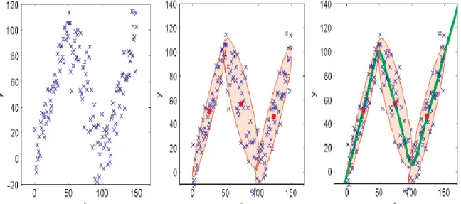
Figure 2.9 - Illustration of GMR using a simple univariate input and output. Left: Data generated by

adding Gaussian noise to 3 linear functions. Middle: A GMM consisting of K=3 components is estimated using the EM algorithm with K-means initialization, mean values are marked as red dots.

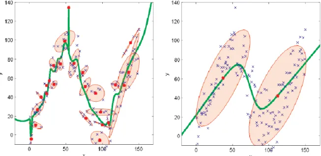
Right: GMR estimation of the expected value of y (green line). ………. 22 Figure 2.10 – Illustration of GMR using different number of components. Data is the same as in figure

2.9. Left: The GMM has been estimated using 25 components (over-fitting). Right: The GMM has been estimated using 2 components (under-fitting)……… 23

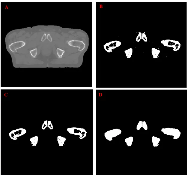
Figure 3.1- Representation of the derivation of the CT bone binary mask. Figure 3.1-A represents the

CT image. Figure 3.1 -B represents the bone binary mask after the thresholding. Figure 3.1-C represents the binary mask after the removal of the spurious objects and figure 3.1-D represents the final bone binary mask after the morphological hole filling operation………. ………… 25

Figure 3.2 – Workflow of the masking in MR features………. 27 Figure 3.3 – Bone segmentation according the IP image using Mevislab. Purple structures represent the

segmented bony tissues………... 28

Figure 3.4 – Workflow of model selection and pseudo-CT construction in the bone using a GMR

procedure. The left side of the scheme represents the pseudo-CT construction using a model which doesn´t include neighbourhood information, while in the right side, the workflow of generating a bone pseudo-CT through a model which includes neighbourhood information is explained……… 30

Figure 3.5 – Illustration of the workflow to obtain the final pseudo-CT. After estimating the dual-model

regression parameters for soft and bony tissues, the resulting pseudo-CTs were overlapped. After, a Gaussian filter is applied for smoothing. ………..…………. 31

ix

Figure 4.1 – Illustration of the results obtained through the water-fat decomposition algorithm without

R2* estimation. Figure 4.1-A represents the fat image, figure 4.1-B the water image with the green line representing the effects of the eddy currents and figure 4.1-C illustrates the obtained field map. All these images are from patient 2……….. 33

Figure 4.2- Illustration of NSA maps obtained for patient 2 when the water-fat decomposition algorithm

is performed without R2* estimation. Figure 4.2-A represents the NSA map of the fat image, while

figure 4.2-B represents the NSA map of the water image……….. 34 Figure 4.3 – Illustration of R2* map of patient 2. The R2* values are described in terms of ms-1

………... 34

Figure 4.4 - Illustration of the results obtained through the water-fat decomposition algorithm with R2* estimation. Figure 4.4-A represents the fat image, figure 4.4-B the water image. Figure 4-C illustrates the obtained R2* map, while figure 4-D represents the obtained field map. All these images are from patient 2………. 36

Figure 4.5- NSA maps of water and fat images of patient 2 when a water-fat decomposition with R2*

estimation algorithm is performed. Figure 4.5-A represents the NSA map of the fat image, while figure

4.5-B illustrates the NSA map of the water image………. 37 Figure 4.6 – Illustration of the fat fraction images obtained for patient 2. Figure 4.6-A represents the

fat fraction obtained using a noise correction approach, while figure 4.6-B doesn’t include the correction of the noise. Figure C illustrates the absolute difference between figure A and 4.6-B………. 38

Figure 4.7 – Representation of in-phase mage obtained for patient 2 in Figure 4.7-A. The green line

represents a row where the signal profile is represented in Figure 4.7-B. As it can be seen the outer edges of the bone structure crossed by the green line are clearly distinguishable from the surrounding tissue, allowing the bone segmentation ……… ………. 38

Figure 4.8 – Bone dice score per patient between the bone MR segmentation and the CT bony tissues

……… 39

Figure 4.9 – Joint histogram between the fat fraction values and the HU values in soft tissue

……… 40

Figure 4.10 – Representation of the values of MAE in soft tissue. Figure 4.10-A represents the MAE

of each patient while Figure 4.10-B represents the average MAE per polynomial order………... 41

Figure 4.11 – Illustration of the pseudo-CT for soft tissue of patient 3. The black areas inside the body

represent bony tissues ……… 41

Figure 4.12 – Representation of AIC values for each model using different number of Gaussians in

GMR. For Model I, the variability present in the model is sufficiently explained by a combination of two gaussians, while for Model II, three gaussians are required to explain its variability. ………... 42

Figure 4.13 – Representation of the MAE for bony tissues using different models. Figure 4.13-A

x using each model for bony tissues HU estimation. As it is possible to see, Model II exhibits superior predicting performance in terms of MAE for all the patients used in this study………... 43

Figure 4.14 – Illustration of the pseudo-CT obtained for bony tissues of patient 3………. 43 Figure 4.15 – Representation of the obtained pseudo-CTs (first column, figures A, D, G, J, M), the

corresponding CT slices (second column, figures B, E, H, K, N) and the absolute difference between the pseudo-CT and CT (third column, figures C, F, I, L, O). The first three rows represent transverse slices for patient 3,5 and 6, respectively. The fourth and fifth rows represent sagittal and coronal slices from patient 5, respectively. The upper scale bar belongs to the pseudo-CT and the real CT whereas the lower belongs to the absolute difference images……… 45

Figure 4.16 – Relation between the MAE and the true CT values, showing that the higher the HU, higher

the MAE, excepting for the air (-1000 HU) which was not considered in the soft tissue regression model……….. 46

Figure 4.17 – Mean Absolute Error between the pseudo-CT and CT before and after the application of

the Gaussian filter. Figure 4.17-A represents the MAE in the body for all the patients, while figure

4.17-B represents the MAE in bony tissue for all the

patients……… ………...46

Figure 4.18-A and figure 4.18-B – Representation of the obtained value for each patient of the SSIM

and the PSNR, respectively, before and after the application of the Gaussian filter ……… 47

Figure 4.19 – Joint histogram between the true CT number and the predicted CT number. The green

line represents the ideal scenario where the pseudo-CT is exactly equal to the real CT. Points below this line indicate a higher HU in the real CT compared to the pseudo-CT, while points above indicate a higher HU in the pseudo-CT compared to the real CT. ………. 48

xi

Contents

List of Figures ... viii

1. Introduction ... 1

2. Background ... 4

2.1. CT imaging ... 4

2.2. MR Imaging ... 5

2.2.1. Physical Principles ... 5

2.2.2. Fat and water Magnetic Resonance Imaging ... 9

2.2.2.1. Physics of water-fat imaging ... 10

2.2.2.1.1. NMR Spectrum of water and fat ... 10

2.2.2.1.2. B0 Inhomogeneities ... 10

2.2.2.2. Water-Fat Separation Techniques ... 11

2.2.2.2.1. Chemical shift based water-fat separation ... 11

2.2.2.2.1.1. Graph Cut Water-Fat decomposition algorithm ... 12

2.2.2.2.1.2. Fat Fraction ... 14

2.3. Estimating HU values from MR data ... 14

2.3.1. Anatomy-based methods ... 15

2.3.1.1. Atlas-based method ... 15

2.3.1.2. Patch-based method ... 16

2.3.2. Voxel-based methods ... 17

2.3.2.1. Manual Bulk Density Assignment ... 17

2.3.2.2. Direct Voxelwise Conversion ... 17

2.4. Gaussian Mixture Regression ... 20

2.4.1. Gaussian Mixture Model ... 20

2.4.2. Regression using a Gaussian Mixture Model ... 21

2.4.3. Impact of changing the number of components ... 22

3. Methods and Materials ... 24

3.1. Data Specification ... 24

3.1.1. CT acquisition ... 24

xii

3.2. MR/CT Registration ... 24

3.3. Water/Fat Decomposition and R2* estimation ... 26

3.4. MR and CT masking ... 27

3.5. Pseudo-CT generation and Validation... 28

3.5.1. MRI bone segmentation ... 28

3.5.2. Soft tissue HU conversion model ... 29

3.5.3. HU conversion model for bone anatomy ... 29

3.5.4. Final Pseudo-CT generation and metrics of evaluation ... 31

4. Results and Discussion ... 33

4.1. Water-Fat Decomposition and R2* estimation ... 33

4.2. Pseudo-CT generation ... 39

4.2.1. MRI bone segmentation ... 39

4.2.2. Soft tissue HU conversion model ... 39

4.2.3. HU conversion model for bone anatomy ... 41

4.2.4. Final pseudo-CT generation and evaluation ... 43

5. Conclusions and Future Work ... 49

References ... 51

Appendix ... 57

1

Chapter 1

Introduction

Computed tomography (CT), with its high availability and geometric accuracy, has proven to be an invaluable tool for many clinical applications where radiation transport simulation is necessary. Since the voxel’s intensity of a CT image is related to the tissue electron density, CT images may be used to quantify the attenuation of X-rays within a tissue, which, in turn, is necessary to simulate radiation transport. For this reason, CT is considered as the golden standard technique of both radiotherapy planning (RTP) and attenuation correction of Positron Emission Tomography (PET) images [1] [2]_.

Despite the many advantages of CT, Magnetic Resonance Imaging (MRI) is starting to replace the use of CT in some applications, mainly due to improved soft tissue contrast and the lack of ionizing radiation.

PET-MRI is an emerging technology with enormous potential for improvements over PET-CT for staging, multiparametric therapy planning and functional assessment of treatment response. PET-MRI was shown to outperform PET-CT in the diagnostic and evaluation of some lesions and diseases, such as breast cancer, prostate cancer and the detection of soft tissue lesions in the brain, liver and lymph nodes [3][4] [5]_{. However, current PET-MRI systems lack accurate attenuation correction, which is the}

most significant of all the corrections applied during PET image reconstruction[6] [7] [8][9]_{. Since the MRI}

voxel’s intensity is governed by the proton density and relaxation effects, there is no relation between the MRI voxel’s intensity and the tissue electron density, necessary to perform the attenuation correction[10]_.

MR-based RTP and integrated MRI treatment machines, such as MRI linear accelerator combinations, are another emerging technologies, with the potential to improve tumour visualization during treatment compared to conventional systems that use ionizing radiation[11] [12] [13]_{. Several studies}

have shown the superiority of MRI for contouring tumour and organs at risk volumes in terms of target volume delineation[14] [15] [16]_{. However, similar to the attenuation correction for PET-MRI, radiation}

absorption in tissue depends on photon interaction with electrons, and MRI does not directly relate to such effects.

Traditionally, to overcome these problems, CT is also performed in order to calculate the attenuation correction map as well as the dose to be delivered. However, this practice introduces systematic errors in MRI-CT registration, that will cause ambiguities in the following PET-MRI and MR-RTP procedures. Furthermore, the use of ionizing radiation and the additional costs and scanning time associated with obtaining and using multiple imaging modalities are serious limitations of this practice[17]_.

Thus, the natural follow-up is to completely replace the use of CT by MRI. When residing to MRI-only techniques, there must be an accurate method to derive CT equivalent data from the MR data to be able to perform attenuation correction and dose calculations in the same way as it is done when using a real CT image. MRI-based CT-equivalent images are generally called pseudo-CT images (or synthetic CT or substitute CT). This approach brings many benefits including the reduction of imaging

2 acquisition costs and radiation exposure, as well as the elimination of the registrations errors between different imaging modalities[18]_.

Several methods were developed in order to generate a pseudo-CT, either by using an anatomy-based approach or a voxel-anatomy-based approach. The main challenge for the first case lies in the difficulty of accurate registration when the patient’s geometry is very different from the atlas, which will lead to significant errors. When using a voxel-based approach, one of the main problems is the lack of signal in cortical bone, making it indistinguishable from the air[18]_{. Ultrashort Echo Time (UTE) sequences have}

been proposed to distinguish bone and air[19]_{. However, for areas with a large field of view (FOV), such}

as the pelvic area, difficulties related to the hardware and noise considerations associated with UTE sequences make them unsuitable for clinical application[20]_{. Furthermore, most of these methods also}

acquire different MR sequences in order to obtain different contrasts to generate the pseudo-CT, which leads to an increase in scanning time[21] [22] [23]_.

In this dissertation, we propose to develop a MRI conversion approach for the generation of pseudo-CTs using a combination of an MR-based water-fat decomposition algorithm with a Gaussian mixture regression algorithm for the pelvic area. In this way, the acquisition of different sequences to obtain different contrasts will be replaced by contrasts that could be obtained through post-processing of images from a single acquisition. Specifically, water and fat images may be obtained from a water-fat-decomposition algorithm. Moreover, other semi-quantitative images may be obtained by the conjugation of these two images, such as a fat fraction image, that may provide a different contrast between voxels. Furthermore, as a gradient-echo sequence is used, an estimation of the T2* decay is

possible. In this work, a dual-model regression is applied, with one model applied to soft tissue and the second model tuned to the bone anatomy obtained by segmentation. As soft tissues are mainly constituted by water and fat, the use of a water-fat decomposition scheme seems obvious for the separation of these two species in the MR images, followed by HU values assignment through regression. Regarding the bone anatomy, it was demonstrated the correlation of the T2* decay as well

as proportion of the fat signal in a voxel with the bone mineral density [17][24] [25] [26] [27]_{. Furthermore, the}

correlation between the HU values and the bone mineral density was also demonstrated, with higher bone mineral density tissues, normally caused by the presence of minerals such as calcium, representing denser bones [28]_{. By including the water and fat information together with information about the T}

2*

decay in a Gaussian mixture regression procedure, it is expected to obtain a good estimation of the HU units in the bone anatomy. Also, the influence of including neighbourhood information for HU estimating in the bone anatomy is investigated. This approach was evaluated on six patient datasets for which CT and MR images were available for prostate sites, by using a leave-one-out-cross-validation procedure. The pseudo-CTs were obtained for the six patients and were compared to the corresponding CT images.

The goal of this project was to investigate if the conversion of MR-data into CT equivalent data could be established without prior CT information and by a better fundamental understanding of the MR signal itself, aiming at completely removing CT acquisitions of the traditional workflow of PET-MRI and MR-RTP.

This dissertation describes the work performed at Image Sciences Institute (ISI), part of the University Medical Center (UMC) of Utrecht, The Netherlands, during a 10 months internship. The work is here organized in 5 chapters. Chapter 2 provides background information about CT imaging, MR imaging and MR-based water-fat decomposition, different approaches to derive a pseudo-CT and Gaussian mixture regression. Chapter 3 describes the data, software and methods used in this work.

3 Chapter 4 presents the relevant results and also the discussion. Finally, Chapter 5 summarizes the main conclusions and possible future work.

4

Chapter 2

Background

2.1. CT imaging

In CT, transaxial X-ray projections are computed to create cross-sectional images of the human body. In a CT scanner, the X-ray tube rotates around the body, while the beams pass through the patient at different angles. The intensity of the attenuated beams is measured and then converted into an electric signal using detectors placed on the opposite side of the X-ray tube. After processing, these signals are transformed into attenuation values consisting of the CT raw data[29]_{. This data is then converted into an}

image using one of several possible a CT reconstruction algorithms, of which the filtered back-projection algorithm is the most widely used[30]_{. As a final result, each voxel of the reconstructed CT}

image represents a scanned voxel with a specific Hounsfield Unit (HU), describing the degree of attenuation relative to water[31]_:

HU(i, j) = 1000 × μ(i, j) − μw μw

(2.1)

where μ(i, j) represents the linear attenuation coefficient of the voxel (i, j) and μw is the linear

attenuation coefficient for water at the same spectrum of photon energies.

The HU is a measure that describes the absorption properties of the tissue relative to water. Therefore, different HU values are responsible for creating different contrasts in a CT image, as it can be seen in figure 2.1[31]_{. Generally, bone appears brighter since it has the highest HU values (ranging}

from 400 to 1800 HU), air is black as it presents the smallest HU values (-1000 HU), while soft tissues present different shades of grey according to their HU values[32] [33]_{. The similarity in HU values for}

different soft tissues makes the distinction between tumours and healthy tissues difficult.

5 The accuracy of attenuation correction and dose calculations based on CT images is determined by the precision of HUs to relative electron densities conversion. This relationship is called calibration curve[34]_.

2.2. MR Imaging

2.2.1.

Physical Principles

Due to the magnetic properties of the atomic nuclei, protons and neutrons present a spin angular momentum and an associated magnetic moment 𝜇⃗. In Nuclear Magnetic Resonance (NMR), instead of a single particle, it is important to study all particles[35]_{. Thus, it is important to convert from the magnetic}

momentum of a single particle to a measure that represents the sum of all magnetic momenta. This sum can be represented by a vector called magnetization, 𝑀⃗⃗⃗:

𝑀⃗⃗⃗ = ∑ 𝜇⃗⃗⃗⃗ 𝑖 (2.2)

For NMR’s studies, two components of 𝑀⃗⃗⃗ are important: 𝑀⃗⃗⃗⃗⃗⃗⃗⃗⃗, the transverse magnetization, and 𝑥𝑦

𝑀𝑧

⃗⃗⃗⃗⃗⃗, the longitudinal magnetization. In a state without any external force applied, the magnetic momentum of each particle is random, and therefore 𝑀⃗⃗⃗ is equal to 0, as it can be seen in figure 2.2[35] [36]_.

When an external magnetic field B0 is applied (normally in z-component), the magnetic

momentum of each particle will align with the direction of B0, and therefore the magnetization vector

in the z-direction is not 0, as represented in figure 2.3. For 1_{H, which is the most typical isotope used in}

NMR, only two magnetic momenta are allowed (±1/2) and therefore two energy states are allowed, having the same energy. However, if the proton is placed into B0, the angular momentum will align with

Figure 2.2 – Illustration of a single particle momentum and resulting magnetization vector when there is no external force applied [36].

6 the field direction, making that the resultant magnetic momentum does not have the same energy for both states. The state with the z-component parallel to B0 presents a lower energy than the state with the

z-component anti-parallel. In this way, there are more particles align parallel to B0 than anti-parallel and

𝑀⃗⃗⃗ will be parallel to B0 [36][37].

It is possible that spin transition from one state to the other one happens by supplying energy to the system. This energy has to be equal to the difference of energy of both states. This energy supplying can be done by applying a radio frequency (RF) pulse with frequency equals to

𝜔0= 𝛾𝐵0 (2.3)

Where 𝜔0 is named Larmor frequency and 𝛾 is the gyromagnetic ratio, that is specific to the used

isotope (for 1_{H, γ/2π=43 MHz/T).}

When the RF pulse (B1 field) is applied in the xy-plane with the Larmor frequency, the particles

in the spin-up state can, therefore, transit to the spin-down state. Adding to this effect, the individual particles will rotate (precession movement) in phase (phase coherence) allowing a transverse magnetization to appear, as represented in figure 2.4. Regarding 𝑀⃗⃗⃗, the RF pulse will lead the rotation of this vector, and the angle of rotation (flip angle, α) will only depend on the amplitude of the B1 field

and the duration of the pulse (t):

𝛼 = 𝛾𝐵1𝑡 (2.4)

Figure 2.3 – Illustration of a single particle momentum and resulting magnetization vector when there B0 magnetic field is

7 As the RF pulse is stopped, the particles return to the rest state as well as 𝑀⃗⃗⃗. For this to happen, the particles emit a RF wave with the Larmor frequency, called the free inductive decay (FID). The return to the equilibrium state is called relaxation and is governed by two physical phenomena: spin-lattice relaxation and spin-spin relaxation[36][37] [38]_.

As the spins return to the spin-up state, 𝑀⃗⃗⃗⃗⃗⃗ returns to the rest state (spin-lattice relaxation) due to 𝑧

energy dissipation to the spins’ surroundings. This process is called T1 recovery, described by

𝑀𝑍 = 𝑀0 (1 − 𝑒−𝑡/𝑇1) (2.5)

Where 𝑀0 is the magnetization at t=0, and T1 is the spin-lattice relaxation time or longitudinal

time.

Moreover, after stimulation, the net magnetization starts to dephase (spin-spin relaxation), due to the inhomogeneities of B0 and the interaction between the spins. This process is called T2 decay and it

is described by

𝑀𝑥𝑦= 𝑀𝑥𝑦0 𝑒−𝑡/𝑇2 (2.6)

Where T2 is the spin-spin relaxation time or transverse relaxation time.

Although relaxation is the result of stochastic processes, some deterministic conditions, such as the inhomogeneity of B0, causes different spins to precess with different resonance frequencies. The B0

inhomogeneities may be caused by the presence of mineral such as iron and calcium, that create distortion in B0[37]. Thus, the spins will dephase, causing the decay of the total transversal magnetization.

In this way, the effective transversal relaxation time will be referred as T2* and it is defined as

1 𝑇₂∗= 1 𝑇2 + 1 𝑇₂′ (2.7)

Figure 2.4 – Illustration of a single particle momentum and resulting magnetization vector when the RF-pulse (B1 field) is

8 Where T2 is the stochastic contribution and T2’ the deterministic. By definition, T2* is always

shorter than T2.

T1, T2 and T2* relaxation times are dependent on the material composition and consequently also

the acquired NMR signal.

However, as the FID signal quickly vanishes due to the T2* decay, it is difficult to acquire.

Therefore, MRI pulse sequences are used for rephasing the spins. The coherent signal that is emitted after rephasing is designed by echo. In practice, the pulse sequences are always repeated with a fixed repetition time (TR) in order to reduce the noise and to achieve different space encoding in the different repetitions. There are two fundamental types of MR pulse sequences: Spin Echo (SE) and Gradient Echo (GE) sequences[37]_{. The remaining developed MR sequences derive in some way from the combination}

of the SE and GE sequences.

In a SE sequence, after applying a 90° RF-pulse, the transversal magnetization will decay exponentially according to T2*, due to differences in the frequency precession of different spins. If a

second RF-pulse with a flip angle of 180° is applied, all spins will rotate 180° around the direction of the B1 field, causing the inversion of the relative phases of the spins in the transversal plane, while the

longitudinal magnetization continues unchanged. In this way, faster spins that were leading in-phase will now be lagging in phase. After the 180° pulse, these spins will catch up with the slower spins, causing the rephasing of the spins. This rephasing results in an echo signal. The time between the 90° pulse and the emission of the echo is called echo time (TE) [37]_.

Gradient echo sequences are created using a magnetic field gradient instead of a RF-pulse. After the excitation pulse, typically smaller than 90°, a gradient is switched on, causing the dephasing of the spins. Then, the polarity of the gradient is reversed, causing the spins’ rephasing and the formation of an echo. As the spins’ rephasing occurs only with respect to the gradient, and not to other sources of dephasing, the signal amplitude is dependent on the T2* decay[37].

This T2* decay can be quantified in GE sequences using:

1

𝑇₂∗= 𝑅2∗= −

log 𝑆(𝑇𝐸𝑛) − log 𝑆(𝑇𝐸1)

𝑇𝐸𝑛− 𝑇𝐸1

(2.8)

where 𝑆(𝑇𝐸𝑛) is the signal intensity when the TE was equal to the nth echo of the acquisition,

𝑇𝐸𝑛 is the echo time of the nth echo of the acquisition. 𝑆(𝑇𝐸1) is the signal intensity of the first echo of

the acquisition acquired at 𝑇𝐸1.

In this way, MR intensities can be correlated with proton densities, which are related to the number of hydrogen atoms in a volume, and tissue relaxation properties rather than with the attenuation properties of the tissues such as in CT. The density and relaxation time of protons in different tissues is used to create the required contrast and signal intensity for diagnostic purpose in MR images by changes in TE and TR. The contrasts are created based on a linear look up table, where magnitudes of the measured signals are converted to a grey tone.

Thus, there are 3 different types of contrasts in MR images that can be created by changing TE and TR: T2-weighted images, T1- weighted images and proton-density (PD) weighted images[39]. In T2

-weighted images, the TR and TE are both long and tissues with long T2, such as fluids, present the highest signal intensities, producing a bright appearance. T2 images are often called as “pathology

images” as the abnormal fluids appear bright against the dark normal tissue. In T1-weighted images,

9 short T1 values, such as fat based tissues. This contrast can be achieved by using short TR and TE. T1

images are often called anatomy scans as they display clearly the boundaries between different tissues. PD-weighted images give a quantitative summary of the number of protons per unit tissue. The higher the number of protons in a tissue, the brighter the tissue will appear on the image. This contrast can be achieved by using a long TR and a short TE[39]_.

As for CT, MRI generates cross-sectional images of the human body. The RF pulse is therefore delivered only to the slice that is needed to be imaged. Slice position will be selected according to the central frequency of the applied RF pulse. After selecting slice thickness and position, the spatial position of the MR signal needs to be identified which is accomplished using spatial encoding. Spatial encoding comprises two steps, phase encoding and frequency encoding, requiring the application of additional gradients that will change the magnetic field strength along the x and y axis enabling unique spatial identification of each voxel. The raw-data space which is used to store the digitized MR signals during acquisition is called k-space. The k-space has two axes with the horizontal axis (kx) representing

the frequency information and the vertical axis (ky) the phase information. The final MR image will be

created from the raw data by applying the 2D- Fourier Transformation to the k-space after the scan is over[39]_.

2.2.2.

Fat and water Magnetic Resonance Imaging

Most clinical magnetic resonance imaging applications detect the signal from protons, which compromise over 90% of nuclei in the human body. The detected protons are either part of water, bound to molecules or carbohydrates, or fat. Their respective signal intensities in imaging voxels results from a combination of their spin density, longitudinal and transverse relaxation times (T1 and T2,

respectively), and the parameters of the imaging sequence used. By exploiting the particular characteristics of hydrogen, MRI can provide excellent contrast between soft tissue, according to whether they are bound to water or lipid molecules[40]_.

With its relatively short T1 relaxation time, fat signal often appears bright in many important

clinical imaging sequences and can obscure underlying pathology such as edema, inflammation, or enhancing tumours. For this reason, water-fat decomposition methods are necessary to supress or detect fat signal and improve visualization of these abnormalities[40]_.

Several techniques of water-fat decomposition were proposed such as the chemical shift saturation pulse and the short-tau inversion recovery (STIR). In the first technique, a frequency selective RF pulse and a spoiler gradient pulse are used in conjunction to first excite and then saturate the fat magnetization before water is excited during imaging[41]_{. In STIR, the longitudinal magnetization of fat}

is first flipped 180° by an inversion pulse and then allowed to relax back to its equilibrium along the magnetic field direction. Water magnetization, which is usually also flipped 180° by the same inversion pulse, is excited when the longitudinal magnetization of fat crosses the null point. Due to the short T1

relaxation time of fat, water has usually relaxed only partially along the longitudinal axis at the time of excitation[42] [43]_.

Although the previous techniques can obtain a reliable fat suppression, for pseudo-CT generation purposes, detection rather than suppression is more valuable, once quantification of water and fat is necessary, since they present different HU values, as it can be seen in figure 2.1. Also, it was demonstrated that the quantitative fat fraction is correlated with bone mineral density, which is correlated with the HU values of bone[26] [28]_.

10 In this way, methods that could quantify the signal of water and fat are preferred over suppression techniques. These methods that are able to perform separation as well as quantification are referred as chemical shift water-fat decomposition techniques[40] [44]_.

2.2.2.1. Physics of water-fat imaging

2.2.2.1.1.

NMR Spectrum of water and fat

The electronic shielding of the protons in fat molecules is greater than that experienced by protons in water molecules, resulting in different microscopic magnetic fields, and subsequently different proton resonance frequencies. Fat has a complex spectrum with multiple peaks, the largest of which is shifted downfield by ≈ 3.5 ppm from the water peak[40] [45]_.

The resulting chemical shift, Δfcs in the resonance frequency is linearly related to the magnetic

field strength B0:

∆𝑓𝑐𝑠=

𝛾

2𝜋𝐵0 × ∆𝛿 [𝑝𝑝𝑚] ×10

−6 (2.9)

As the chemical shift is directly proportional to B0, the chemical shift at 1.5 T is -210 Hz (fat

precesses slower than water), while at 3 T, it doubles to -420 Hz at body temperature (37°C), as represented in figure 2.5[46]_.

2.2.2.1.2.

B

Inhomogeneities

Most of the water-fat separation techniques rely on the assumption that there are constant frequencies for fat and water across the image. However, in practical applications many factors can create inhomogeneities in the B0 field that violate this assumption and result in imperfection suppression

of fat[40]_.

Although the main magnet itself may have an imperfect magnetic homogeneity, this is a minor effect since modern MR scanners are shimmed to homogeneity within 1 ppm across the field of view (FOV). Magnetic susceptibility introduced by the patient leads to more significative B0 inhomogeneities

and it can be caused by several sources, such as air/tissue interfaces, ears or the bowel gas. These B0

Figure 2.5 – Illustration of the resonance spectrum of water and fat at 3 Tesla. The stars represent the additional peaks of fat [40].

11 inhomogeneities have three main effects: distortion in the readout gradient, accelerated T2* decay for

gradient echo imaging and failed fat suppression which is the most relevant for the context of this work[40]_.

2.2.2.2. Water-Fat Separation Techniques

2.2.2.2.1.

Chemical shift based water-fat separation

Chemical shift based water-fat separation methods comprise a class of approaches commonly known as “Dixon” water-fat separation. As for the frequency selective approach, the Dixon techniques rely on the water-fat chemical shift difference. However, the Dixon techniques encode the chemical shift difference into the signal difference with a modified data acquisition and then achieve the water/fat separation through post-processing. In its original approach, Dixon acquired an image with water and fat signal in-phase and another image with the signal 180° out-of-phase[44] [47]_{. The choice of the echo}

times to achieve these two images is done using

𝑇𝐸 = 𝜃

2𝜋 ∆𝑓𝑐𝑠

(2.10)

where θ is the phase shift between water and fat signal. In this way, the Dixon technique can be described by the following equation system:

{𝐼𝑃 = 𝑊 + 𝐹 𝑂𝑃 = 𝑊 − 𝐹 <=> { 𝑊 =(𝐼𝑃 + 𝑂𝑃) 2 𝐹 =(𝐼𝑃 − 𝑂𝑃) 2 (2.11)

where IPrepresents the in-phase image, OP the out-of-phase image, F the fat image and W the water image. As this approach only requires two images, it is considered a “two-point” method.

Unfortunately, Dixon’s original approach was sensitive to B0 inhomogeneities that resulted in

water-fat swapping in the image[40]_{. Thus, this approach was subsequently modified to include a third}

image that was used to compensate for B0 inhomogeneities. This three-point method acquire images at

TE values that generate phase shifts of 0, +π and -π between the water and fat[48]_{. The additional}

information can be used to calculate a B0 field inhomogeneity map (field map). By using phase

unwrapping algorithms, this approach is able to remove the effects of field distortions, thereby avoiding water-fat swapping, turning this method more robust[44] [49] [50]_{. However, this technique increases the}

scan time and doesn’t allow flexibility in the sequence design since the images have to be acquired at specific TE values[40]_.

To allow more flexibility in the pulse sequence design and, consequently, reduce the scan time, several methods were developed that allow arbitrary TE values to accomplishing the water-fat separation, such as the iterative decomposition of water and fat with echo asymmetry and least squares estimation (IDEAL)[51]_{. This method uses images acquired at arbitrary TE values together with an}

iterative least square estimation of the field map to accomplish a voxel-independent water-fat separation. However, in areas with severe field inhomogeneities this method still fails to obtain an accurate field map since, with this technique, the field map can be directly estimated only if the true field map ranges between ± Δfcs/2. In practice, the field inhomogeneity may exceed this range[52]. Furthermore, these

12 the echo spacing. The use of this alternating bipolar gradient turns the estimation of the field map susceptible to eddy-currents, which manifest itself as phase errors[53] [54] [55]_.

More recently, a water-fat separation method that uses a graph-cut algorithm to jointly estimate water/fat images and the field map was proposed[56]_{. In this approach, the estimation of the field map at}

all voxels is formulated as the minimization of a global criterion, which is the linear combination of the sum of the voxel-independent criteria and a field map smoothing penalty, and solve it using an iterative graph cut algorithm. This algorithm is further explained below.

2.2.2.2.1.1.

Graph Cut Water-Fat decomposition algorithm

The graph cut water-fat estimation algorithm uses a multi-echo water and fat decomposition scheme, where a sequence of images is collected with different echo time shifts, t1, t2, tn. The signal at

each individual voxel is described by the following model[51] [56]_:

𝑠(𝑟, 𝑡𝑛) = (𝜌𝑤𝑎𝑡𝑒𝑟(𝑟) + 𝜌𝑓𝑎𝑡(𝑟)𝑒𝑗2𝜋∆𝑓𝑐𝑠𝑡𝑛)𝑒−𝜑(𝑟)𝑡𝑛, 𝑛 = 1, … , 𝑁 (2.12)

where ρwater(r) and ρfat(r) are complex-valued concentrations of water and fat, respectively. The

field map, f(r), is consolidated in 𝜑(𝑟) through

𝜑(𝑟) = [𝑗2𝜋 f(𝑟)] (2.13)

From this signal model, it is possible to observe that there are 2 complex unknows, ρwater(r) and ρfat(r), and 1 real unknown, f(r), in a total of 5 (each complex unknown has a real and imaginary

unknown). As each image contributes with a real and imaginary measurement, constituting two measurements per TE value, at least 3 images at different TE values have to be acquired, since the number of measurements has to be always equal or higher than the number of unknown parameters.

Also, in this signal model, it is assumed that fat only presents a single resonance frequency. However, fat has several peaks. In particular, the spectral peak from olefinic proton (5.3 ppm) is close to the water resonance frequency, which can cause some water-fat swapping[57]_{. One possible solution}

is to include in the signal model a weighted sum of the amplitudes of the fat peaks, by changing equation 2.12 to:

𝑠(𝑟, 𝑡𝑛) = (𝜌𝑤𝑎𝑡𝑒𝑟(𝑟) + 𝜌𝑓𝑎𝑡(𝑟) [∑ 𝛽𝑖𝑒𝑗2𝜋∆𝑓𝑐𝑠𝑖𝑡𝑛 𝑀

𝑖=1

]) 𝑒−𝜑(𝑟)𝑡𝑛_{, 𝑛 = 1, … , 𝑁 (2.14)}

Here, the fat signal is modelled using an M (usually 6) peak model, where ∆𝑓_𝑐𝑠𝑖 is the chemical shift between the ith _{fat peak and water (Hz), and β}

i >0 is the relative weight of each peak. However, this

model would require N ≥ M+2 images to estimate the unknown parameters, which is not practical due to the increased scan time. In this way, it is assumed that βi are known. Thus, the number of unknown parameters remains the same as the single peak model[56] [57]_{. Consequently, only 3 images have to be}

acquired.

However, this multi-peak signal model doesn’t account for T2* decay. Although for many

applications the T2* decay may be neglected, for imaging with substantially shortened T2*, it is

important to consider the effects from both fat and T2*, as they may interfere with the estimation of each

13 model[57] [58]_{. This can be done by modelling the B}

0 field inhomogeneity and the T2* decay in a complex

field map term, by changing equation 2.13 to:

𝜑(𝑟) = [1 𝑇⁄ 2∗(𝑟)− 𝑗2𝜋𝑓(𝑟)]

(2.15)

In this way, the number of unknown parameters increases to 6, thus 3 images acquired at different TE values should be enough for obtaining all the unknown parameters. However, as the number of complex acquired images is equal to the number of unknown parameters, the estimation can be very sensitive to noise. For a better performance, typically 6 echoes are acquired. Furthermore, for pseudo-CT generation, besides the importance of the R2* estimation for water-fat decomposition, some studies

prove the correlation between R2* values and HU values, especially in bone tissues. This is mainly due

to the correlation between R2* values and bone mineral density, since bone minerals as calcium create

local inhomogeneities that are reflected by R2* values [27].

The model in equation 2.14 can be written in a matrix form as:

[ 𝑒−(𝜑(𝑟)𝑡1) _𝑒−(𝜑(𝑟)𝑡1)_{(∑ 𝛽} 𝑖𝑒−𝑗2𝜋𝛿𝑖𝑡1 𝑀 𝑖=1 ) 𝑒−(𝜑(𝑟)𝑡𝑛) _𝑒−(𝜑(𝑟)𝑡𝑛)_{(∑ 𝛽} 𝑖𝑒−𝑗2𝜋𝛿𝑖𝑡𝑛 𝑀 𝑖=1 ) ] ⏟ 𝐴_𝜑 ∗ [𝜌_𝜌𝑤𝑎𝑡𝑒𝑟 𝑓𝑎𝑡 ] ⏟ 𝑔 = [𝑠[1] 𝑠[𝑁]] ⏟ 𝑠 (2.16)

The unknown parameters are obtained by minimizing the least-square errors between the model and the measured data:

{𝜌𝑤𝑎𝑡𝑒𝑟, 𝜌𝑓𝑎𝑡, 𝜑} = arg min

𝜌𝑤𝑎𝑡𝑒𝑟,𝜌𝑓𝑎𝑡,𝜑‖𝐴𝜑

𝑔 − 𝑠‖2 (2.17)

Since the above minimization is dependent on many parameters, the criterion is minimized with respect to some variables by assuming the other to be fixed, thus eliminating them from the optimization[59]_{. Minimizing the above cost function with respect to the concentrations, assuming ϕ to}

be fixed, we obtain the optimal concentration estimates as 𝑔𝑜𝑝𝑡 = (𝐴𝜑𝑇𝐴𝜑)−1𝐴𝜑𝑇𝑠. Replacing the

optimal concentrations back in the previous cost function, and solving for ϕ, we obtain 𝜑(𝑟) = arg min 𝜑 ‖𝐴𝜑(𝐴𝜑 𝑇_𝐴 𝜑) −1 𝐴𝜑𝑇𝑠(𝑟) − 𝑠(𝑟)‖ ⏟ 𝐶(𝑟,𝜑) 2 (2.18)

In case of necessity of R2* estimation, again it is possible to minimize the expression with respect

to T2* to obtain a cost function that is only dependent on f:

𝑓(𝑟) = arg min

𝑓 min_⏟ 𝑇₂∗ 𝐶(𝑟, 𝜑) 𝐷(𝑟,𝑓)

(2.19)

Since the estimation of T2* values doesn’t suffer from ambiguities, an exhaustive search over

14 In order to address the sensitivity of the voxel-by-voxel optimization strategy described in equation 2.19 to multiple feasible solutions and phase wrapping, the joint recovery of the field map is formulated as a smoothness regularized optimization scheme. The global criterion is the linear combination of the sum of D and a smoothness penalty:

𝑓̂ = 𝑎𝑟𝑔 min 𝑓 ∑ 𝐷(𝑟, 𝑓(𝑟)) 𝑟 + 𝜇 ∑ ∑ 𝜔𝑟,𝑠 |𝑓(𝑟) − 𝑓(𝑠)| ℵ(𝑟) 𝑟 (2.20)

Here, ℵ(r) is the local neighbourhood of the voxel at location r, μ is an additional smoothing constant and ωr,s are pre-defined weights that specify the relative importance of each difference term.

The first term of equation 2.20 is the sum of the voxel independent criteria in equation 2.19, while the second term promotes field map smoothness. Then, the continuous problem is converted to a discrete optimization scheme by restricting the field map to a set of discrete values.

However, the direct discrete minimization of equation 2.20 is computationally infeasible, since it involves a large and fully connected graph, an iterative scheme where a one-layer graph is constructed and a sequence of binary decision problems at each iteration[60]_{. These decision problems are solved}

efficiently using a s-t graph cut algorithm. Thus, at (n+1)th _{iteration, there are two possible solutions at}

each voxel:Γ𝑛+1(𝑟) = {𝑓𝑛(𝑟), 𝑔𝑛(𝑟)} . Here, 𝑓𝑛(𝑟) is the optimal solution obtained from the previous

iteration, while 𝑔𝑛(𝑟) is chosen as 𝑓𝑛(𝑟) ± 𝛽, where 𝛽 may be a pre-specified constant, or a picked

randomly among a set of local minimizers of D. This binary decision problem is efficiently solved using a s-t graph-cut algorithm[61]_{, guarantying the solution to converge to a global minimum, obtaining in this}

way the field map (and, if it is the case, the R2* map). Uploading this into the signal model represented

by equation 2.14, it is possible to obtain the water and fat images.

2.2.2.2.1.2.

Fat Fraction

As already discussed, quantification of the fat signal is important for pseudo-CT generation. The quantification can be done by calculating the relative amount of fat in a voxel[62]_{, by using}

𝐹𝐹 = 𝐹

𝐹 + 𝑊 ×100

(2.21)

where FF refers to fat fraction, F and W to the fat and water signal in a voxel, respectively. Thus, the FF will present values between 0 and 100. However, if the true fat content is 0, any noise in the fat estimate will result in an FF>0. Thus, FF will be biased by noise[63]_{. This can be avoided}

by calculating the fat fraction as[55]_:

𝐹𝐹 = { 𝐹 𝐹 + 𝑊 ×100 𝑖𝑓 𝑊 < 𝐹 (1 − 𝑊 𝐹 + 𝑊) ×100 𝑖𝑓 𝑊 > 𝐹 (2.22)

2.3. Estimating HU values from MR data

As previously mentioned, PET-MRI and MR-RTP lack electron density information to perform attenuation correction and dose calculations. This problem is commonly solved by the acquisition of an additional CT scan, which leads to systematic errors in the workflow caused by the imperfect MR-CT

15 registration. Thus, the estimation of HU values from MR data is a crucial step in PET-MRI and MR-RTP workflow.

Several approaches were developed to solve this problem. It is possible to group the several approaches into two main groups: anatomy-based approaches and voxel-based approaches[18]_{. The}

anatomy-based method generally uses a non-rigid registration between a library of MR reference images and a new patient MRI to warp a reference CT to match the anatomy of the new patient data[64] [65] [66] [67]_{. This method leads to significant errors when the new patient MRI geometry is very different}

compared to the geometry of the MR atlas[18]_{. The voxel-based method could be divided into two types.}

The first one involves a direct characterization into different tissue classes by manual segmentation followed by bulk assignments of HU values[68] [69]_{. The second one comprises a direct conversion of}

MRI voxels values to HU values by introducing a prior correlation between MRI and CT [17] [22] [23] [70] [71]_.

2.3.1.

Anatomy-based methods

The anatomy-based method could be divided into two main approaches: the atlas-based method[64] [65] [66] [66] _{and the patch-based method}[72]_.

2.3.1.1.

Atlas-based method

The atlas-based method uses information from the whole image and can be divided in 3 steps, as illustrated in figure 2.6:

1. First, every CT and MR image from the atlas dataset are aligned using non-deformable registration (elastic deformation) to enable intra-subject alignment and producing multiple conjugated CT-MR atlas image pairs[64] [66]_.

2. Then, a registration between all MR atlas images and the MRI of a new patient is performed using non-deformable and deformable transformations, enabling the alignment between the MRI of the new patient and the MR atlas[64] [65]_.

3. The transformation matrices and deformation fields used in step 2 are also applied to the CT images in the atlas, building the pseudo-CT, according to different strategies of atlas fusion for HU value assignment [64] [65]_.

16 The HU value for each voxel in the obtained pseudo-CT can be obtained using a simple mean process[64] [66] _{or a weighted average based on similarity measures}[67]_.

Using a simple mean process, the pseudo-CT intensity (μ) of a voxel at the position x0 is calculated

using the mean of those at the same location in all deformed CT images in the CT atlas[64]_:

𝜇(𝑥0) = 1 𝑁𝑎× ∑ 𝑦𝑖(𝑥0) 𝑁𝑎 𝑖=1 (2.23)

Where Na is the number of atlases and yi the HU value in all CT images in the atlas.

In the weighted average based on similarity measures method, the MRI of the new patient is matched with the MRI atlas database using deformable registration and local image similarity measures such as the local sum of squared differences (NSSD) and the structural similarity index extended to regions of interest (ROI-SSIM). The similarity results are ranked across all MR images in the atlas according to the quality of the registration. The ranks in each nth _{subject and each voxel 𝑣⃗, 𝑅}

𝑛𝑣⃗⃗, are then

converted to weights, 𝑊𝑛𝑣⃗⃗. Better registration results lead to a higher weight by applying a negative

exponential decay function[67]_:

𝑊𝑛𝑣⃗⃗ = 𝑒−𝛽×𝑅𝑛𝑣⃗⃗⃗ (2.24)

Where β is a constant weighting factor. Then the intensity at each voxel of the pseudo-CT is calculated using 𝐼_𝑣⃗⃗𝑝𝐶𝑇=∑ 𝑊𝑛𝑣⃗⃗×𝐽𝑛𝑣⃗⃗ 𝐶𝑇 𝑁𝑎 𝑛=1 ∑𝑁𝑎𝑛=1𝑊𝑛𝑣⃗⃗ (2.25)

Where 𝐽_𝑛𝑣𝐶𝑇_⃗⃗ is the atlas CT image from subject n at voxel 𝑣⃗.

2.3.1.2.

Patch-based method

The patch-based method involves the use of a rigidly aligned CT-MRI atlas as database but it excludes the use of deformable registrations. In this method, 3D patches are extracted from the target MRI followed by a spatial local search of the most intensity similar patches in the MRI database[72]_.

Thus, the use of deformable registrations is replaced by the patch resemblance search.

The patches extracted from the MRI atlas are centred on an arbitrary spatial location x, PS(x), and

the HU value on position x in the aligned CT is designed by TS(x). Then, using this database, an intensity

based nearest neighbour search is performed using:

𝑑(𝑠, 𝑥) = ‖𝑃(𝑦) − 𝑃𝑆(𝑥)‖2 (2.26)

where P(y) represents the patch at the target MRI. Then, the search is done aiming at finding the patch that minimizes 𝑑(𝑠, 𝑥). After this search, the corresponding HU value in the CT atlas at the same spatial location is stored as 𝑇_𝑠𝑘𝑚𝑖𝑛(𝑥_𝑘𝑚𝑖𝑛). Then, the HU value in the pseudo-CT at position y is

calculated using a weighted average:

𝑝𝐶𝑇(𝑦) =∑ 𝑤𝑘×𝑇𝑠𝑘𝑚𝑖𝑛(𝑥𝑘

𝑚𝑖𝑛₎ 𝑘

∑ 𝑤𝑘 𝑘