‘r
Costa de Caparica 201X
The Analysis of
Complex Adaptive Systems
Method SBCANAL
Second edition
Luís Soares Barreto
Costa de Caparica
2019
CAS
Without text
CAS
The Analysis of
Complex Adaptie Systems
Method SBCANAL
The Analysis of CAS
The Analysis of
Complex Adaptie Systems
Method SBCANAL
Second edition
Luís Soares Barreto
Jubilee Professor of Forestry University of Lisbon Portugal© Luís Soares Barreto, 2018, 2019
The Analysis of Complex Adaptie Systems. Method SBCANAL
Second editon
E-book published by the author
htp://hdl.handle.net/10400.5/1 5100Prof. Doutor Luís Soares Barreto
Av. do Movimento das Forças Armadas, 41 – 3D 2825-372 Costa de Caparica
Portugal
With compliments
This e-book is free ware but neither public domain nor open to changes. It can be copied and freely disseminated only in its to-tality, with respect for the authorship rights. It can not be sold.
Dedicaton
To Sandra Isabel, and Luísa Maria
I am grateful to those who contribute
to the existence of ClickCharts, LibreOfce, Maxima,
R, Scilab e wxMaxima
The author
Luís Soares Barreto was borne in 1935, in Chinde, a small
village in the delta of the Zambezi River, in Mozambique.
In this African country, from 1962 tll 1974, he did research
in forestry, and he was also member of the faculty of the
Universidade de Lourenço Marques (actual Universidade
Eduardo Mondlane, Maputo), where he started the
teach-ing of Forestry. While member of this university, from
1967 to 1970, he was a graduate student at Duke
Univer-sity, Durham, NC, U.S.A.. From this univerUniver-sity, he
re-ceived his Master of Forestry in Forest Ecology
(1968), and his Ph. D. in Operatons Research applied to
Forestry (1970). Since 1975 tll March, 2005, he taught at
the Insttuto Superior de Agronomia, Universidade de
Lis-boa. From 1975 to 1982, simultaneously, he taught in the
Department of Environmental Sciences of the Universidade
Nova de Lisboa. Here, in 1977, he conceived, and created
a new fve years degree in environmental engineering. He
is the only Portuguese who established a scientfc theory.
Besides the ecological theory presented in this book, he
proposed also a unifed theory for forest stands of any kind
and ecologically sound management practces grounded
on it. The later theory is a partcular case of the former
one. Actually, the author is jubilee professor of the
Univer-sity of Lisbon.
Other books by the author
:
Madeiras Ultramarinas. Insttuto de Investgação Cientfca de Moçambique, Lourenço Marques, 1963.
A Produtiidade Primária Líquida da Terra. Secretaria de Estado do Ambiente, Lisboa, 1977. O Ambiente e a Economia. Secretaria de Estado do Ambiente, Lisboa, 1977.
Um Noio Método para a Elaboração de Tabelas de Produção. Aplicação ao Pinhal. Serviço
Nacional de Parques, Reservas e Conservação da Natureza, Lisboa 1987.
A Floresta. Estrutura e Funcionamento. Serviço Nacional de Parques, Reservas e Conservação da Natureza, Lisboa, 1988.
Alto Fuste Regular. Instrumentos para a sua Gestão. Publicações Ciência e Vida, Lda., Lisboa,
1994.
Étca Ambiental. Uma Anotação Introdutória. Publicações Ciência e Vida, Lda., Lisboa, 1994.
Poioamentos Jardinados. Instrumentos para a sua Gestão. Publicações Ciência e Vida, Lda.,
Lisboa, 1995.
Pinhais Mansos. Ecologia e Gestão. Estação Florestal Nacional, Lisboa, 2000.
Pinhais Braios. Ecologia e Gestão. E-book, Lisbon, 2005. htp://hdl.handle.net/10400.5/14258 Theoretcal Ecology. A Unifed Approach. E-book, Lisbon, 2005.
Iniciação ao Scilab. E-book, Lisbon, 2008
Áriores e Arioredos. Geometria e Dinâmica. E-book, Costa de Caparica, 2010. htp:// hdl.handle.net/10400.5/14229
From Trees to Forests. A Unifed Theory. E-book, Costa de Caparica, 2011. htp://hdl.handle.net/ 10400.5/14230
Iniciação ao Scilab. Second editon. E-book, Costa de Caparica, 2011. htp://hdl.handle.net/ 10400.5/14259
Ecologia Teórica. Uma Outra Explanação. I - Populações Isoladas. E-book, Costa de Caparica,
2013. htp://hdl.handle.net/10400.5/14231
Ecologia Teórica. Uma Outra Explanação. II - Interações entre Populações. E-book, Costa de Capa-rica, 2014. htp://hdl.handle.net/10400.5/14231
Ecologia Teórica. Uma Outra Explanação. III – Comunidade e Ecossistema. E-book, Costa de Capa-rica, 2016. htp://hdl.handle.net/10400.5/142 31
TheoretcalEcology. A Unifed Approach. Second editon. E-book, Costa de Caparica, 2017. htp:// hdl.handle.net/10400.5/14 1 75
Contents
Sumário
Cover...1
CAS...2
CAS...3
The Analysis of...3
The Analysis of CAS...4
The Analysis of...5
© Luís Soares Barreto, 2018, 2019...6
The Analysis of Complex Adaptve Systems. Method SBCANAL...6
Dedicaton...7
CAS...8
The author...9
Other books by the author:...10
Contents...11
A Note on the Second Editon...13
1. Introducton...15
1.1. The Scope of this Book...15
1.2. A Sketch of the Explanatory Strategy...15
1.3. The Book...17
1.4. References...17
2. A System of Omnivory...19
2.1 Direct, Indirect, and Total Efects...19
2.2 The Matrix of Total Efects...21
2.3 A Model for Omnivory...23
2.4 References...31
3 SBCANAL: A Procedure to Analyse CAS...33
3.1 Introducton...33
3.2 The Procedure...33
3.3 References...34
4 Identficaton of Keystone Species, and Controlling Components in the Ecosystem...37
4.1 Introducton...37
4.3 The Identfcaton of Keystone Species...40
4.4 The Identfcaton of Controlling Components in Ecosystems...43
4.5 Conclusive Remarks...44
4.6 References, and Related Bibliography...45
5 Developmental, Structural, and Functonal Sensitvites to Inital Values...47
5.1 Introducton...47
5.2 Ascendency...47
5.3 Analysis...57
5.4 Conclusion...58
5.5 References, and Related Bibliography...58
6 Klein’s Data of the US Economy...61
6.1 Introducton...61
6.1 Applicaton of SBCANAL...61
6.2 Interpretaton...66
6.3 References...67
7. The Portuguese Market of Electricity...69
7.1 Introducton...69
7.2 The Data...69
7.3 The Applicaton of Method SBCANAL...69
7.4 Interpretaton...77
7.5 References...77
8. Final Comments...79
8.1. The Nature of Complex Systems...79
8.2 Epistemological aspects...79
8.3 References...80
A Note on the Second Edition
The main changes of this second editon of the book are the following ones:
• I improve fgure 2.2.
• I illustrate the deducton of the matrix of total efects (secton 2.2).
• I show that the functonal structure of systems, and the basic strategy to analyse them are
available since the XVII century (secton 2.3).
1. Introduction
1.1. The Scope of this Book
This book is a spillover of the method I introduced in Barreto (2017: chapters 17, and 18) to identfy keystone species, and controlling factors in ecosystems. The same method is also capable of the appraisal of the developmental, structural, and functonal sensitvites of the system relat-ively to its components. The scope of this text is to show that the method is applicable to other complex adaptve systems (CAS).
If the reader is not familiar with the topic of complexity, and the concept of CAS there is plethora of informaton about the subject available in the internet, such as the entries in the Wikipedia.
Mitchell (2009: 13) defnes succinctly CAS as: “A system that exhibits non trivial emergent and self-organizing behaviours”.
The state of the art on the subject of complex systems can be found in Naciri and Tkiouat (2015). An accessible introductory text to complexity is Mitchell ( 2009). A more embracing per-spectve of complex systems can be found in Hooker (2011).
The complex systems approach is applied in :
• physics • ecology • biology • social sciences • forestry • economics • patern formaton • collectve moton • business management
For related references see table 2 in Naciri and Tkiouat (2015).
The use of the expression complexity science is commented by Professor Melanie Mitchell (Portland State University, and Santa Fe Insttute – the sanctuary of complexity) as fol-lows:
“But how can there be a science of complexity when there is no agreed-on quanttatve defniton of complexityv
I have two answers to this queston. First, neither a single science of complexity nor a single complexity theory exists yet, in spite of the many artcles and books that have used this terms.” (Mitchell, 2009: 13-14).
Actually, the method more used to study CAS is individual (or agent) based modelling (e.g., Grimm, and Railsback, 2005). See also Niazi (2013, and references herewith).
Despite the increasing use of agent based models, the interpretaton, and analysis of their outputs are conspicuously unsatsfactory (Ju-Sung Lee, Tatana Filatova, Arika Ligmann-Zielinska, Behrooz Hassani-Mahmooei, Forrest Stonedahl, Iris Lorscheid, Alexey Voinov, Gary Polhill, Zhan-liSun and Dawn C. Parker, 2015). Thus, any efort to contribute to the analysis of CAS is clearly jus-tfed.
1.2. A Sketch of the Explanatory Strategy
A1. High mutability derived from its adaptability A2. High connectvity related to its complexity
A1 suggests that the study of real CAS must be sustained by tme series covering a large period of tme.
A2 advises the use of models that for each variable accommodates the maximum number of potental interactons. This purpose can be atained applying iector autoregressiie models (VAR) also named multiariate autoregressiie models (MAR).
High connectvity associated with high number of components give origin to an intricate web of indirect efects. Thus, ultmately, the behaviour of the CAS is the refecton of the acton of the total or net efects that emerge. Consequently, the analysis of CAS must be focused on the study of the matrix of total efects. Ahead, we will be more specifc about this issue.
These three paragraphs encapsulate the essental of the procedure we purpose for the analysis of CAS.
In the subsequent text, frst we show that models of systems of ODE can produce simu-lated data that mirror the acton of both direct, and indirect efects, and the method to obtain total efects produces coherent results. For this purpose we use a system of omnivory.
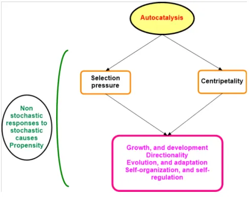
In the possession of a reliable matrix of total efects, we call the concept of autocatalysis ( Ulanowicz , 1997, 2009) to support a method concentrated on the analysis of the matrix of the total positive efects. In fgure 1.1, we atempt a fguratve synthesis of the concept of autocata-lysis.
Figure 1.1. Atempt to synthesize the causal chain related to autocatalysis. Main source of this fgure is Ulanowicz (2009)
Briefy, the core of the analysis of a CAS is the analysis of the network associated to the matrix of the total positve efects that emerges from its dynamics.
1.3. The Book
Referring to the areas were the existence of CAS emerge, we will not be exhaustve. The CAS used to illustrate the applicability of the method of analysis are from ecology, and economics.
In chapter 2,we use a simple system from ecology (omnivory) to illustrate the correctness of the frst part of the proposed method to analyse CAS, this is, the obtenton of a credible mat-rix of total efects.
Chapter 3 is dedicated to the presentaton of method SBCANAL, for the analysis of CAS. In chapter 4, I apply SBCANAL to ecological CAS. We verify the adequacy of the method to identfy keystone species, and controlling factors in ecosystems.
In chapter 5 we widen the signifcance of the results given by SBCANAL. Chapter 6 is devoted to the analysis of a macroeconomic CAS.
In chapter 7 the proposed method is applied to the analysis of the Portuguese market of electricity.
Chapter 8 is dedicated to conclusive remarks.
For easier control we insert in the text the adequate R scripts.
1.4. References
Barreto, L. S., 2017. Theoretcal Ecology. A Unified Approach. Second editon. E-book, Costa de Caparica. htp:// hdl.handle.net/10400.5/14 1 75
Grimm, V., and S. F. Railsback. 2005. Indiiidual Based Modeling and Ecology. Princeton University Press. Mitchell, M., 2009. Complexity. A Guided Tour. Oxford University Press.
Hooker, C., Editor, 2011. Philosophy of Complex Systems. Elsevier.
Ju-Sung Lee, Tatana Filatova, Arika Ligmann-Zielinska, Behrooz Hassani-Mahmooei, Forrest Stonedahl, Iris Lorscheid, Alexey Voinov, Gary Polhill, ZhanliSun and Dawn C. Parker, 2015. The Complexites of Agent-Based Model-ing Output Analysis. Journal of Artficial Societes and Social Simulaton 18 (4) 4.
<htp://jasss.soc.surrey.ac.uk/18/4/4.html> DOI: 10.18564/jasss.2897
Naciri, N., and M. Tkiouat, 2015. Complex System Theory Development. Internatonal Journal of Latest Research in
Science and Technology, 4(6):93-103. ISSN (Online):2278-5299
Niazi, M. A., 2013. Complex Adaptve Systems Modeling: A multdisciplinary Roadmap. Complex Adaptie Systems Modeling 2013, 1:1
htp://www.casmodeling.com/content/1/1/1
Ulanowicz, R. E., 1997. Ecology, the Ascendent Perspectie. Columbia University Press, New York
Ulanowicz, R.E., 2009. Autocatalysis. Em S. E. Jørgensen, (Main editor), Ecosystem Ecology. Elsevier, Amsterdam. Pages 41-43.
2. A System of Omnivory
2.1 Direct, Indirect, and Total Effects
In the social, and fnancial sphere, we are all familiar with chain efects triggered by a single event or measure adopted by a government. The European Central Bank maintains a low rate of interest, and buy natonal debt of some countries because it assumes that this measures trigger a net of interrelated efects that favours the economies of the European countries. We are all fa-miliar with the following causal chain:
increasing the income of citzens → increases consumpton → increases investment in produc-ton of goods for the consumers → increase employment ..
This example is a very simple causal chain. Real systems are much more complex and the task of economists are much more difcult and plagued with disagreement. What makes the understanding of the behaviour of complex systems (as ecosystems, and natonal economies) in-tricate, and their dynamics almost unpredictable beyond a short period of tme, are the rich network of direct, and indirect efects (those mediated by a third component).
Let us introduce an example that will be numerically illustrated ahead. Consider the fol-lowing chain of omnivory:
Figure 2.1. Diagrammatc representaton of omnivory. Populatons as: y1 is the plant; y2 is the herbivore; y3 is the
omnivore
The omnivore y3 has a negatve direct efect on plant y1, and a positve indirect efect
be-cause it diminishes the number of herbivores y2 that also consume the plant.
The total efect (TE) of y3 on y1 is the sum of the direct, and indirect efects: Total or net efeet oo 3 on 1= Direet efeet oo 3 on 1 + indireet efeet oo 3 on 1
If y3 has a very small consumpton of y1, y2 grazes y1 intensively, and y3 consumes
intens-ively y2, the total efect of y3 on y1 may be positve.
On the other side, If y3 has a heavy consumpton of y1, y2 grazes y1 lightly, and y3 consumes
lightly y2, the total efect of y3 on y1 may be negatve.
In an ecosystem, the community is the set of all populatons of the species present in the ecosystem.
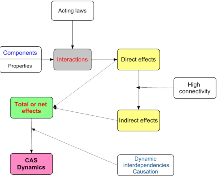
Tentatvely, let me introduce an ontological interpretaton (fgure 2.2).
The direct efects are controlled by the propertes of the components. These propertes determine the kind of interactons that relate the components to each other.
Interactons are indispensable for the existence of systems, causality, identty, and unity. Interactons are ubiquitous from social sciences to theoretcal physics.
Interactons are constrained by laws (e.g., physical, chemical, allometric) actuatng in each given situaton, and give origin to direct efects. From direct efects and high connectvity emerge indirect efects. Total efects are the sum or balance of direct, and indirect efects.
It is the network of TE that controls the system. We can add the efects of the environ-mental factors on the system, and arrive to a similar conclusion: the network of TE controls the system (CAS).
Figure 2.2. Simplifed conjecture about the dynamics of CAS
In fgure 2.2, the chain components→ interactons → direct efects is reductonist but the chain direct efects → high connectvity → indirect efects is holistc. To clarify the dynamics of CAS we must use both approaches.
In the XVII century, Blaise Pascal, in his Pensées, (Pascal, 1958: Secton II, subsecton 72)" already wrote:
“...I hold it equally impossible to know the parts without knowing the whole, and to know the whole without knowing the parts in detail.”
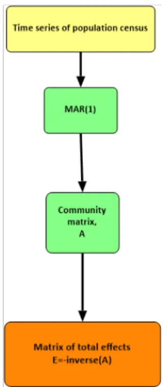
From fgure 2.2, we also conclude that if we want to understand CAS we must fnd a pro-cedure to estmate TE. It is at this point that MAR(1) reveal their utlity.
2.2 The Matrix of Total Effects
A procedure to calculate the total efect of species yj on species yi is to verify how this
spe-cies responds to the introducton of individuals of spespe-cies yj in the system.
To illustrate this statement, let us use model BACO3 (Barreto, 2017: chapter 11) for inter-specifc competton. The ordinary diferental equatons of this model are modifed forms of the ODE for the Gompertz equaton (e.g., Barreto, 2017: chapter 4). To the intraspecifc compet-ton, we add the interspecifc competton. Let us assume the presence of three compettors, yi,
i=1,2,3. Then, the model is writen as:
) ln ln ln (ln 1 11 1 12 2 13 3 1 1 1 yc y a y a y a y dt dy f (2.1) ) ln ln ln (ln 2 21 1 22 2 23 3 2 2 2 y c y a y a y a y dt dy f (2.2) ) ln ln ln (ln 3 31 1 32 2 33 3 3 3 3 yc y a y a y a y dt dy f (2.3) Being yif, the fnal sizes of the populatons, when the species grow isolated. In a fxed point
it is verifed: 3 13 2 12 1 11 1 ln ln ln ln 0 y f a y a y a y (2.4) 3 23 2 22 1 21 2 ln ln ln ln 0 y f a y a y a y (2.5) 3 33 2 32 1 31 3 ln ln ln ln 0 y f a y a y a y (2.6)
Now, we introduce perturbaton I2=1, in the equaton of species y2. The system moves to
a new equilibrium y*i, i=1,2,3. To calculate the alteratons caused by perturbaton I2 we
diferentate the equatons with respect to I2, at the new equilibrium (yif are constants):
3 1 2 2 1 ) ( 0 j j j I I y a (2.7) 1 ) ( 0 3 1 2 2 2
j j j I I y a (2.8)
3 1 2 2 3 ) ( 0 j j j I I y a (2.9)Let us now use the matrix form of our problem, for easier soluton. The competton coefcients aij are the elements of matrix A.
2 2 3 2 2 2 2 2 1 ) ( ) ( ) ( 0 1 0 I I y I I y I I y A (2.10) From this equaton we obtain:
0 1 0 ) ( ) ( ) ( 2 2 3 2 2 2 2 2 1 E I I y I I y I I y (2.11) Where E=-A-1. To have the inverse, matrix A must be nonsingular(determinant diferent
from zero). Matrix E is the matrix of total efects, and matrix A is the community matrix.
Matrix E says that the total efect caused by the additon of one individual of species 2 on the new equilibrium of species 1 is:
12 1 12 2 2 1( ) (a ) e I I y (2.12) In this equaton, -(a12)-1 is the element of line i, and column j of matrix -A-1.
Generically, the total efect caused by the additon of one individual of species j (column of matrix E) in the new equilibrium of specie i (line of matrix E) is:
ij ij j j i e a I I y 1 ) ( ) ( (2.13) Recapitulatng, if we construct a matrix with the coefcients of the multvariate linear models suggested in secton 1.2, we have the community matrix A. To obtain the matrix of total efects E:
• We calculate the inverse of matrix A;
•The inverse matrix is multplied by -1 to obtain the matrix of total efects E.
Let eij be the element of line i, and column j of E. The element eij is the total efect of
spe-cies j (column) on spespe-cies i (row).
Now we apply these concepts to a system of omnivory.
2.3 A Model for Omnivory
The model for omnivory is an extension of model SBPRED for predaton (Barreto, 2016: secton 18.4). This model exhibits two ODE that are modifed forms of the ODE of theGompertz equa-ton. The equaton for the resource is:
(2.14)
Gompertz equaton Consumpton by the consumer
K is the carrying capacity, asymptotc or fnal value of y1. The speed of growth is
determ-ined by the parameter c1.
The expression for the consumpton is called the hyperbolic or Holling type 2 functonal response, and it is multplied by the number of consumers y2. The greater is a, the area of
dis-covery, the greater is the consumpton. The handling tme of the resource, h, is the tme re-quired to dominate, eat, and digest the prey, before the consumer start searching another prey. The greater is h, the smaller is the consumpton per tme unit.
The ODE for the consumer, y2, is:
(2.15) The carrying capacity of the predator is equal to the number of prey multplied by the parameter b, that mirrors the contributon of each prey to the carrying capacity of the predator (K2=by1). The parameter b depends on the parameters of the functonal response, and the
ef-ciency of the predator on transforming the preys in its own growth Now we can introduce the model to omnivory.
2.3.1 Assumptons
Let us approach the interacton of omnivory represented in fgures 2.2. We assume the following:
The basal species (y1) is a plant that only plays the role of resource;
The middle species (y2) is a herbivore that plays both the role of consumer, and resource;
2.3.2 The Model The model is writen as:
(2.16) (2.17) (2.18) For easier reference I call this model PANT3.
2.3.3 Model Analysis
PANT3 has not an explicit soluton, thus we will use a numerical approach.
This model evinces stable fxed points, and periodic solutons. Now let us illustrate the concepts of the previous secton, using R:
>
> library(deSolve) > library(rootSolve) Warning message:
package ‘rootSolve’ was built under R version 3.3.2 > library(MASS)
>
> ############ Parameters
> c1=0.05; k1=80; a1=1; h1=1; a2=.8; h2=1; c2=0.1 > b1=.4; a3=0.6; h3=0.7; c3=0.15; b2=.3; b3=.2
> #**************** para obter comensalismo presa-omniv subir a1 de 1 para 8 >
> #*************** Model, and solution > baco3<-function(times,y,parms) { + n<-y + + + + dn1.dt<- c1*n[1]*(log(k1)-log(n[1]))-a1*n[1]*n[2]/(1+a1*h1*n[1])-a2*n[1]*n[3]/(1+a2*h2*n[1]+a3*h3*n[2]) + dn2.dt<- c2*n[2]*(log(b1*n[1])-log(n[2]))-a3*n[2]*n[3]/(1+a2*h2*n[1]+a3*h3*n[2]) + dn3.dt<- c3*n[3]*(log(b2*n[1]+b3*n[2])-log(n[3])) + return(list(c(dn1.dt,dn2.dt,dn3.dt))) + } > > > > initialn<-c(2, 0.5, 0.8) > t.s<- seq(1,300, by=0.1) > >
> out<- ode(y=initialn, times=t.s, baco3, parms=parms) >
>
> matplot(out[,1], out[,-1], type="l", col=1, xlab="Time", ylab="Biomass",ylim=c(0,3))
> title("Omnivory")
> legend('topright',paste(rev(r)),lty=3:1,col=1, bty='n') > We obtain fgure 2.3. > #Fixed point > y<-initialn > ST2 <- runsteady(y=y,func=baco3,parms=parms,times=c(0,5000)) > ye<-ST2$y > ye [1] 1.0750756 0.1435188 0.3512265 Fixed point
> #Preparing data to fit MAR(1) > h<-out[,-1] > > g<-seq(1,2991,10) > dat0<-matrix(c(h[g,]),300,3) > N1<-dat0[,1] > N2<-dat0[,2] > N3<-dat0[,3] > ###################################### >
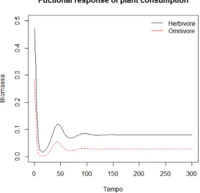
> ## Functional responses of plant consumption >
> rf1=a1*N1*N2/(1+a1*h1*N1)
> rf2=a2*N1*N2/(1+a2*h2*N1+a3*h3*N2) > rf=matrix(c(rf1,rf2),nrow=300, ncol=2) >
> matplot(rf, type="l", col=1:2, xlab="Tempo", ylab="Biomassa",ylim=c(0,0.5)) >
> title("Fuctional response of plant consumption") > r<-c('Herbivore','Omnivore') > legend('topright',paste(r),lty=1,col=1:2, bty='n') We obtain fgure 2.4. > ###### MAR(1) > > m<-c(dim(dat0)) > N1a<-N1[-1] > N1b<-N1[-m[1]] > N2a<-N2[-1] > N2b<-N2[-m[1]] > N3a<-N3[-1] > N3b<-N3[-m[1]] > > fit1<-lm(N1a ~ N1b+N2b+N3b) > fit2=lm(N2a ~ N1b+N2b+N3b) > fit3=lm(N3a ~ N1b+N2b+N3b) > summary(fit1) Call: lm(formula = N1a ~ N1b + N2b + N3b) Residuals:
Min 1Q Median 3Q Max -0.0187033 -0.0005764 -0.0005748 -0.0005692 0.0176170 Coefficients:
(Intercept) 0.147109 0.002704 54.398 < 2e-16 *** N1b 1.031816 0.002032 507.672 < 2e-16 *** N2b -0.984843 0.024103 -40.859 < 2e-16 *** N3b -0.112166 0.013577 -8.261 4.93e-15 *** ---Signif. codes: 0 ‘***’ 0.001 ‘**’ 0.01 ‘*’ 0.05 ‘.’ 0.1 ‘ ’ 1 Residual standard error: 0.003742 on 295 degrees of freedom Multiple R-squared: 0.999, Adjusted R-squared: 0.999 F-statistic: 1.025e+05 on 3 and 295 DF, p-value: < 2.2e-16
> summary(fit2)
Call:
lm(formula = N2a ~ N1b + N2b + N3b) Residuals:
Min 1Q Median 3Q Max -0.0030700 0.0000033 0.0000037 0.0000049 0.0040778 Coefficients:
Estimate Std. Error t value Pr(>|t|) (Intercept) 0.0113767 0.0003498 32.53 <2e-16 *** N1b 0.0283827 0.0002629 107.98 <2e-16 *** N2b 0.7648236 0.0031173 245.35 <2e-16 *** N3b -0.0231806 0.0017560 -13.20 <2e-16 *** ---Signif. codes: 0 ‘***’ 0.001 ‘**’ 0.01 ‘*’ 0.05 ‘.’ 0.1 ‘ ’ 1 Residual standard error: 0.0004839 on 295 degrees of freedom Multiple R-squared: 0.9997, Adjusted R-squared: 0.9997 F-statistic: 3.044e+05 on 3 and 295 DF, p-value: < 2.2e-16
> summary(fit3)
Call:
lm(formula = N3a ~ N1b + N2b + N3b) Residuals:
Min 1Q Median 3Q Max -0.0041753 0.0001649 0.0001662 0.0001670 0.0023129 Coefficients:
Estimate Std. Error t value Pr(>|t|) (Intercept) 0.0020775 0.0006634 3.131 0.00191 ** N1b 0.0563517 0.0004986 113.016 < 2e-16 *** N2b -0.0001651 0.0059132 -0.028 0.97775 N3b 0.8211913 0.0033309 246.535 < 2e-16 *** ---Signif. codes: 0 ‘***’ 0.001 ‘**’ 0.01 ‘*’ 0.05 ‘.’ 0.1 ‘ ’ 1 Residual standard error: 0.0009179 on 295 degrees of freedom Multiple R-squared: 0.9997, Adjusted R-squared: 0.9997 F-statistic: 2.95e+05 on 3 and 295 DF, p-value: < 2.2e-16 >
>
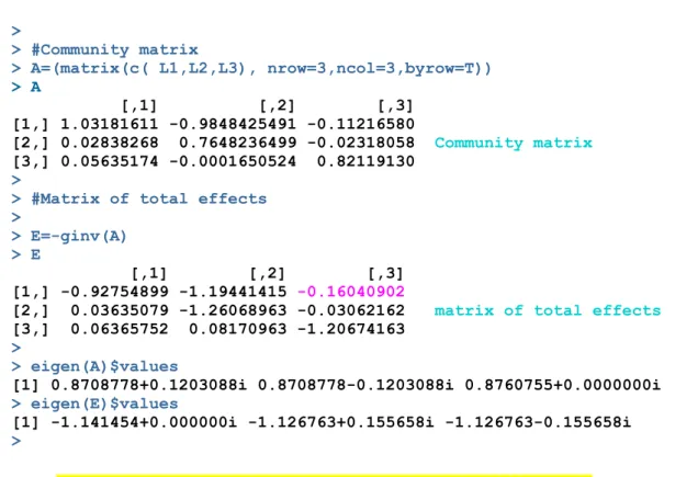
> L1=coef(fit1)[-1] > L2=coef(fit2)[-1] > L3=coef(fit3)[-1]
> > #Community matrix > A=(matrix(c( L1,L2,L3), nrow=3,ncol=3,byrow=T)) > A [,1] [,2] [,3] [1,] 1.03181611 -0.9848425491 -0.11216580 [2,] 0.02838268 0.7648236499 -0.02318058 Community matrix [3,] 0.05635174 -0.0001650524 0.82119130 >
> #Matrix of total effects >
> E=-ginv(A) > E
[,1] [,2] [,3] [1,] -0.92754899 -1.19441415 -0.16040902
[2,] 0.03635079 -1.26068963 -0.03062162 matrix of total effects
[3,] 0.06365752 0.08170963 -1.20674163
>
> eigen(A)$values
[1] 0.8708778+0.1203088i 0.8708778-0.1203088i 0.8760755+0.0000000i
> eigen(E)$values
[1] -1.141454+0.000000i -1.126763+0.155658i -1.126763-0.155658i
>
The omnivore has a negatve total efect on the plant (e13=-0.1604).
The dominant eigenvalue of matrix A close to 1 (0.876) mirror the statonarity of the fxed point of the system. The negatve real part of the eigenvalues of the TE matrix (E) refects the stability of the soluton.
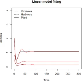
> ############# Simulation with MAR(1) > > bc4<-function(N) { + + N1.t1<-coef(fit1)[1]+A[1,1]*N[1]+A[1,2]*N[2]+A[1,3]*N[3] + N2.t1<-coef(fit2)[1]+A[2,1]*N[1]+A[2,2]*N[2]+A[2,3]*N[3] + N3.t1<-coef(fit3)[1]+A[3,1]*N[1]+A[3,2]*N[2]+A[3,3]*N[3] + + c(N1.t1, N2.t1,N3.t1) + } > > > t<-300 > > N<-matrix(NA,nrow=t+1, ncol=3) > N[1, ]<-c(2, 0.5, 0.8)
> for (i in 1:t) N[i+1, ]<-bc4(N[i, ]) >
> matplot(0:t, N, type='l', col=1, ylim=c(0,4), xlab="Time", ylab="Biomass",) > lines(N1b, col='red')
> lines(N2b, col='red') > lines(N3b, col='red')
> title("Linear model fitting")
> r<-c('Plant','Herbivore','Omnivore')
> legend('topleft',paste(rev(r)),lty=3:1,col=1, bty='n') >
Figure 2.3. Simulaton of the dynamics of model PANT3
Figure 2.5. Populaton dynamics with MAR(1), and model PANT3 (red line)
Now we assume that the area of discovery of the herbivore is not 1 but 8 (a1=8). Let us see what happens to the system.
The dynamics of the system is evinced in fgure 2.6.
Figure 2.6. Simulaton of the dynamics of model PANT3, with a1=8
The fxed point is now y1= 0.51215076, y2=0.09995082, y3= 0.17363530. The consumpton
Figure 2.7. Dynamics of the plant consumpton, in the simulaton with model PANT3, with a1=8
The new community, and total efects matrices are:
> #Community matrix > A=(matrix(c( L1,L2,L3), nrow=3,ncol=3,byrow=T)) > A [,1] [,2] [,3] [1,] 1.16972321 -2.6493694 0.48446100 [2,] 0.03915076 0.7286820 -0.02593494 [3,] 0.05062359 0.2389646 0.69399462 >
> ##Matrix of total effects > > E=-ginv(A) > E [,1] [,2] [,3] [1,] -0.77454315 -2.9571862 0.43017840 [2,] 0.04309751 -1.1911807 -0.07460039 Matrix E [3,] 0.04165936 0.6258743 -1.44662551
Now, with a very voracious herbivore, the omnivore has a positve total efect on the plant (e13=0.43017840).
Model PANT3, and the used analytcal procedure evinced satsfactory sensitvity, and coherence.
The problem of obtaining matrix E is solved with a trustul soluton.
Let us examine matrix E, in the output of the previous R script. All elements of matrix E are non zero. This is, each species is simultaneous cause (column), and efect (line). It is this web of mutual causal relatons that render systems less prone to a simple analysis. This situaton is more acute when systems have a large number of components.
More than three centuries ago, Blaise Pascal had already depicted this duality of roles in nature. For him, it is this duality that justfy the fail of the analysis of systems adoptng only a reductonist or only a holistc approach, as stated in his previous quotaton. Now, we can introduce the complete thought of Pascal (previous quotaton in brown):
“Since everything then is cause and efect, dependent and supportng, mediate and immediate, and all is held together by a natural though imperceptble chain, which binds together things most distant and most diferent, I hold it equally impossible to know the parts without knowing the whole, and to know the whole without knowing the parts in detail.”
The functonal structure of systems, and the basic strategy to analyse them are available since the XVII century.
Pascal’s conjectures were too advanced relatvely to the available mathematcal tools to implement them. Probably, this is the reason why they fell in oblivion. Today, very few scientsts read Pascal’s Pensés.
In fgure 2.8 the fowchart of the analytcal process is exhibited.
Figure 2.8. A fowchart of the method to obtain the matrix of total efects
From here on, the matrix of the coefcients of the MAR will be called community matrix, and will be represented by A. The matrix of total efects is represented by E.
This chapter benefts from Barreto (2017), and Case (2000).
2.4 References
Barreto, L. S., 2016. Ecologia Teórica. Uma Outra Explanação. III – Comunidade e Ecossistema.E-book, Costa de Capari-ca.htp://hdl.handle.net/10400.5/142 31
Barreto, L. S., 2017. Theoretcal Ecology. A Unified Approach. Second editon. E-book, Costa de Caparica. htp:// hdl.handle.net/10400.5/14 1 75
Case, T. J., 2000. An Illustrated Guide to Theoretcal Ecology. Oxford University Press, Oxford, U. K.
3 SBCANAL: A Procedure to Analyse CAS
3.1 Introduction
As already stated in chapter 1, the method here proposed was originated in the area of ecology, and conservaton (Barreto, 2017).
Initally, the method searched a soluton for a problem created by the increasing disrupt-ive efect of humanity on the biosphere. This degrading impact rendered the detecton of key-stone species, and of controlling components of the ecosystem in almost an ethical imperatve for ecologists. It is not surprising that several authors had already approached this subject, such as
Libralato, Christensenc, and Paulyc (2006), Smith et al. (2014), and Zhao et al. (2016). Thus the method was our contributon to the soluton of this problem.
After, successfully, we searched the applicability of the method to other types of CAS. This text is a consequence of this inquiry.
3.2 The Procedure
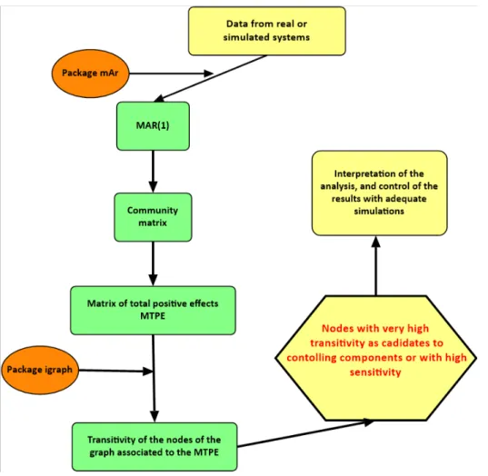
The procedure integrates the following concepts, and models: - CAS can be modelled by MAR(1).
- The concept of autocatalysis (Ulanowicz , 1997, 2009). - The concept of total positve efects (chapter 2).
- The concept of transitvity or clustering coefcient, from network analysis (e.g., Kolaczyk, and. Csárdi, 2014).
The procedure is sustained by the following conjecture:
In the network associated to the matrix of total positie efects (MTPE), the nodes with high transitiity must giie a strong contributon to the process of autocatalysis, and thus they haie high probability of being components to which the CAS is iery sensitie.
Given the tme series of the components of the CAS, the steps of the procedure are the following ones (fgure 3.1):
1. Fit a MAR(1) model to the data;
2. From the matrix of the coefcients extract the matrix of the total positve efects; 3. Use this matrix as a weighted adjacency matrix, and obtain the correspondent network; 4. Calculate the clustering coefcient or transitvity of each node;
5. Select the nodes (components) with high coefcients as candidates to be controlling components of the CAS.
Basically, we apply network analysis not to the data itself, but to the matrix of total positve efects underpinning the data dynamics. The procedure is simultaneously dynamic (MTPE), and statc (network analysis).
For easier reference, this procedure is named SBCANAL .
The analysis of the network associated to the matrix of the total positve efects may have a larger scope then the sole transitvity, and may be object of a more enlarged, and deeper analysis using the available functons in the package igraph or any other similar package available. The extension of the analysis, and the analytcal tools used depend on the kind of CAS, and the purpose of the analysis.
As it will be illustrated ahead, the cluster coefcients of the nodes provide a ranking of the sensitvity of the CAS to the variatons per se of each one of the components of the system. In same situatons this informaton may high valuable.
Figure 3.1. Flowchart of the procedure to analyse CAS, with method SBCANAL
The method reveals a shortcoming: its exigence of tme series of several years. In some area of research, as ecology, more often projects last only 3-4 years. This is seldom enough to obtain a good fing for the VAR model.
Probably, we must revise the funding of ecological projects, as the administratve tme scale is not coincident with the one of some ecological research projects. Otherwise, we will never acquire the informaton we need to successfully overcome the environmental crisis.
3.3 References
Barreto, L. S., 2017. Theoretcal Ecology. A Unified Approach. Second editon. E-book, Costa de Caparica. htp:// hdl.handle.net/10400.5/14 1 75
Kolaczyk, E. D., and G. Csárdi, 2014. Statstcal Analysis of Network Data with R. Springer, Berlin.
Libralato, S., V. Christensenc, and D. Paulyc, 2006. A method for identfying keystone species in food web models.
Smith, C. et al, 2014. Report on identficaton of keystone species and processes across regional seas. Deliverable 6.1, DEVOTES Project. 105 pp + 1, Annex.
Ulanowicz, R. E., 1997. Ecology, the Ascendent Perspectie. Columbia University Press, New York
Ulanowicz, R.E., 2009. Autocatalysis. Em S. E. Jørgensen, (Main editor), Ecosystem Ecology. Elsevier, Amsterdam.
Pages 41-43.
Zhao, L. et al., 2016. Weightng and indirect efects of identfy keystone species in food webs. Ecology Leters, 19:1033-1040.
4 Identification of Keystone Species, and Controlling Components in
the Ecosystem
4.1 Introduction
We were unable to fnd real data, a tme series covering many years (or other tme unit), of an ecosystem or community including a keystone species. Then, we used simulated data to apply the method in the search of keystone species, and real data for the problem of the identfcaton of controlling factors of the ecosystem.
In the next secton we succinctly present the model of ecosystem we use. It is obtained from Barreto (2017: chapters 15 and 16). This reference can consulted for more details.
4.2 The Simulated Ecosystem
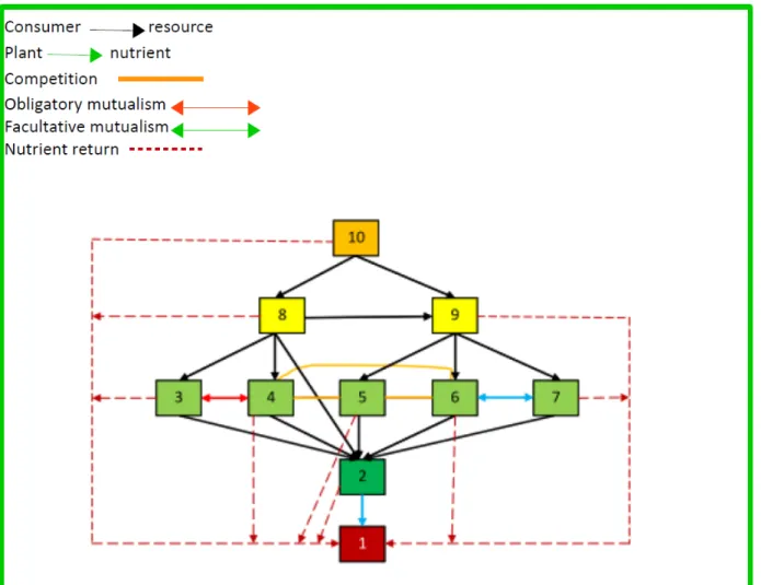
The hypothetcal ecosystem is characterized as follows:
• It has a community with nine populatons;
• The existence of a nutrient that acts as a limitng factor;
• The cycle of the nutrient is closed. In terrestrial ecosystems this can be accepted with any reluctance. For instance, see Chapin III, Matson, and Mooney (2002:220-222).
The interactons present in the community are:
• Herbivory; • Competton; • Facultatve mutualism; • Obligatory mutualism; • Predaton; • Omnivory.
A graphical representaton of the ecosystem is exhibited in fgure 4.1. From fgure 15.3, we can infer the following:
• Variable 1 refers to the nutrient; • Variable 2 refers to the vegetaton; • Species 3 to 7 are herbivores;
• Variable 10 is a top predator (can also be a parasite);
• Specie 8 is omnivore and reveals intra-trophic predaton, as he consumes 9; • There is an interacton of obligatory mutualism between species 3 e 4; • There is an interacton of facultatve mutualism between species 6 e 7;
The size of the populatons are measured using an arbitrary unit of biomass B.
There are more compettve interactons then those represented in fgure 4.1. We sup-pressed them to avoid an almost illegible network. The complementary informaton about the prevailing competton is as follows:
• As the species have a Gompertzian dynamics they are submited to intraspecifc
com-petton;
• The interspecifc competton between herbivores is asymmetric;
• The species of each mutualistc interacton do not compete with each other; • Specie y3 benefts from the presence of species y5, y6, y7;
• Specie y4 benefts from the presence of species y5, y6, y7;
• Specie y5 benefts from the presence of species y6, y7 but is depressed by species y3, y4;
• Specie y7 is depressed by y3, y4, y5.
Figure 4.1. Flowchart of the simulated ecosystem
The following is also assumed:
• All species release 1% of their biomasses to the soil, in unit of tme;
• For each unit of nutrient assimilated by the plant, it produces 1000 units of plant biomass; • The carrying capacity of the plant is 1000 y1;
• The contents of the nutrient in the biomasses are: plant: 0,001; herbivores: 0.01;
omnivore, and predator y9:0,1; top predator:0,3;
• The ODE of the nutrient is equal to the contents of the fallen liter less the plant uptake; • The plant uptake is given by y2*y1/(50+0.4*y1).
The model is described by the following system of 10 ordinary diferental equatons: (4.1) Te=[0.001 0.01 0.01 0.01 0.01 0.01 0.1 0.1 0.3] (4.2) ) 4 . 0 50 ( 01 . 0 1 2 1 10 2 1 y y y y Te dt dy i i
2 2 1 1 2 2 y r(ln(1000y ln y )) ex 0.01y dt dy r1= 0.05
ex<-y2*y3/(70+0.2*y4)+ y4*y2/(90+0.3*y2)+y5*y2/(90+0.3*y2)+y6*y2/(80+0.3*y2)+
+y7*y2/(75+0.3*y2)+y8*y2/(83+0.3*y2)
(4.3) r2= 0.069, b2= 0.2 comp2=0+0+0.02*ln y5+0.03*ln y6+0.04*ln y7 prey7[1]=y8*y3/(50+0.2*y3) (4.4) r3= 0.061, b3= 0.21 comp3=0+0+0.01*ln y5+0.02*ln y6+0.03*ln y7 prey7[2]=y8*y4/(60+0.3*y4) (4.5) r4=0.057, b4= 0.28 comp4=-0.04*ln y3 -0.03*y4+0+0.01*ln y6+0.02*ln y7 prey8[1]=y9*y5/(50+0.21* y5) (4.6) r5= 0.055, b5= 0.29
comp5=-0.04*y3-0.03*y4-0.02y5+0+0
prey8[2]=y9*y6/(60+0.3*y6)
(4.7) r6= 0.05, b6= 0.27
comp6=-0.04*y3-0.03*y4-0.02y5+0+0
prey8[3]=y9*y7/(70+0.3*y7))
(4.8) r7= 0.06, k7= 6.667y2+ 0.0667y3+ 0.070y4
3 2 3 2 2 10 4 3 2 3 r y (8y 10 )(ln(b y ) ln(y comp ) prey7[1] 0.01y dt dy 4 3 4 2 3 10 3 4 3 4 ry (9y 10 )(ln(b y ) ln(y comp ) prey7[2] 0.01y dt dy 5 4 5 2 4 5 4 5 r y (ln(b y ) ln y comp ) prey8[1] 0.01y dt dy 6 5 6 003 . 0 2 5 6 5 6 r y (ln(b y (2 e 7) ln y ) comp ) prey8[2] 0.01y dt dy y 7 6 7 03 . 0 2 6 7 6 7 r y (ln(b y (2 e 7))) ln(y comp ) prey8[3] 0.01y dt dy y 8 8 7 8 7 8 r y (lnk ln y ) prey9[1] 0.01y dt dy
prey9[1]=y10*y8/(30+0.2*y8)
(4.9) r8= 0.035, k8= 0.112y5+ 0.116y6+ 0.108y7
prey9[2]= y10*y9/(40+0.3*y9)
prey7[3]=y8y9(45+0.23*y9))
(4.10) r9= 0.02, k9=0.4535y8+ 0.028y9
If we remove the top predator (y10) from the system it collapses, this is, the answer of the
simulator for the system, in R platorm, is ‘NA’ for the sizes of the other variables. Thus, y10 is a
keystone species.
We showed in Barreto (2017: chapter 16) that MAR(1) can be well fted to the data gen-erated by the simulator of the described ecosystem.
The constructed ecosystem do not pretend to represent any partcular community, and the choice of the interactons only serves to our explanatory purposes. The same is applicable to the parametrisaton of the model.
4.3 The Identification of Keystone Species
To apply SBCANAL to the ecosystem we constructed, the following R script is applied:
> #semomtransBk > library(deSolve) > library(MASS) > library(rootSolve) > > modul<-function(times,y,parms) { + n<-y + + r<-c(0.05, 0.09, 0.071, 0.057, 0.055, 0.07, 0.06, 0.035, 0.02) + b<-c(20, 0.2, 0.21, 0.28, 0.29, 0.27) + b7<-c(b[1], b[2], b[3])/3 + b8<-c(b[4], b[5], b[6])/2.5 + bm7<-mean(b7)/5 + bm8<-mean(b8)/4 + b9<-c(bm7, bm8) + +
+ #plant:consumption of the plant + #herb & omniv
+ ex<-sum( y[2]*y[3]/(70+0.2*y[2]), y[4]*y[2]/(90+0.3*y[2]), y[5]*y[2]/(90+0.3*y[2]), y[6]*y[2]/(80+0.3*y[2]), y[7]*y[2]/(75+0.3*y[2]), y[8]*y[2]/(83+0.3*y[2]))
+
+ #competition and predation of the herbivores
9 9 8 9 8 9 ry (lnk ln y ) prey9[2] prey7[3] 0.01y dt dy 10 10 9 10 9 10 r y (lnk ln y ) 0.01y dt dy
+ #inicial/final<-iniciais/(bi*resouce) +
+ a1n<-c(0, 0, 0.02, 0.03, 0.04)
+ y1n<-log(c(y[3], y[4], y[5], y[6], y[7])) + a2n<-c(0, 0, 0.01, 0.02, 0.03)
+ y2n<-log(c(y[3], y[4], y[5], y[6], y[7])) + a3n<-c(-0.04, -0.03, 0, 0.01, 0.02)
+ y3n<-log(c(y[3], y[4], y[5], y[6], y[7])) + a4n<-c(-0.04, -0.03, -0.02, 0, 0)
+ y4n<-log(c(y[3], y[4], y[5], y[6], y[7])) + a5n<-c(-0.04, -0.03, -0.02, 0, 0)
+ y5n<-log(c(y[3], y[4], y[5], y[6], y[7])) + + #effects of competition + comp2<-sum(a1n*y1n) + comp3<-sum(a2n*y2n) + comp4<-sum(a3n*y3n) + a5n<-c(-0.04, -0.03, -0.02, 0, 0)
+ y5n<-log(c(y[3], y[4], y[5], y[6], y[7])) + comp5<-sum(a4n*y4n)
+ comp6<-sum(a5n*y5n) +
+ +
+ #consumption of predators y[8], y[9] & y[10]
+ prey7<-y[8]*c(y[3]/(50+0.2*y[3]), y[4]/(60+0.3*y[4]), y[9]/(45+0.23*y[9])) + prey8<-y[9]*c(y[5]/(50+0.21*y[5]), y[6]/(60+0.3*y[6]), y[7]/(70+0.3*y[7])) +
+ prey9<-c(y[10]*y[8]/(30+0.2*y[8]), y[10]*y[9]/(40+0.3*y[9])) + #comp. oblig mutual prey
+
+ #carrying capacity of y8
+ k7<-sum(b7*c(y[2], y[3], y[4])); +
+ #carrying capacity of y9
+ k8<-sum(b8*c(y[5], y[6], y[7])) + #carrying capacity of y10
+ k9<-sum(b9*c(y[8], y[9]))
+ #fraction of biomass that falls + fr=0.01
+ biom=c(y[2:10])
+ m=fr*biom # fallen biomass + #nutrient in the biomasses
+ te=c(0.001,rep(0.01,5),rep(0.1,2),0.3) + + #ODE + dy1.dt<-sum(te*m)-y[2]*y[1]/(50+0.4*y[1]) + dy2.dt<-y[2]*r[1]*(log(1000*y[1])-log(y[2]))-ex-m[1] + dy3.dt<-y[3]*r[2]*(8*y[4]-10^(-10))*(log(b[2]*y[2])-log(y[3])+comp2)-prey7[1]-m[2] + dy4.dt<-y[4]*r[3]*(9*y[3]-10^(-10))*(log(b[3]*y[2])-log(y[4])+comp3)-prey7[2]-m[3] + dy5.dt<-y[5]*r[4]*(log(b[4]*y[2])-log(y[5])+comp4)-prey8[1]-m[4] + dy6.dt<-y[6]*r[5]*(log(b[5]*y[2]*(2-exp(-0.003*y[7])))-log(y[6]) +comp5)-prey8[2]-m[5] + dy7.dt<-y[7]*r[6]*(log(b[6]*y[2]*(2-exp(-0.03*y[7])))-log(y[7])+comp6)-prey8[3]-m[6] + dy8.dt<-y[8]*r[7]*(log(k7)-log(y[8]))-prey9[1]-m[7] + dy9.dt<-y[9]*r[8]*(log(k8)-log(y[9]))-prey9[2]-prey7[3]-m[8] + dy10.dt<-y[10]*r[9]*(log(k9)-log(y[10]))-m[9]
+ +
+ return(list(c(dy1.dt,dy2.dt,dy3.dt, dy4.dt, dy5.dt, dy6.dt,dy7.dt,dy8.dt, dy9.dt, dy10.dt))) + } > > #parms<-c(r, b, k) > initials<-c(40, 400, 36, 36, 36, 36, 36, 12, 12, 4) > t.s<- seq(1, 300, by=0.1) > >
> out<- ode(y=initials, times=t.s, modul)
> #matplot(out[,1], out[,-1], type="l", xlab="Tempo", ylab="N") > > > library(MASS) > library(rootSolve) > library(mAr) > > y<-initials > ST2 <- runsteady(y=y,func=modul,parms=parms,times=c(0,5000)) > ye<-ST2$y > ye # Fixed point [1] 0.1590013091 5.0090621641 0.7430847673 0.7773484198 1.2074297620 [6] 1.2346934021 1.2341296936 8.4034232056 0.0002859149 2.3117477578 > > h=out[,-1] > > > g<-seq(1,2991,10) > > M=h[g,] > > y=mAr.est(M,1,1) > y$SBC [1] -15.60132 >
> # matrix of total effects
> E=-ginv(y$AHat) > # METP > AS=E > n=1:10 > for (i in n) { + for (j in n) { + if (AS[i,j]<0) {AS[i,j]=0} + + } + } > rownames(AS)=c('N','V','H1','H2','H3','H4','H5','O','P1','P2')
> colnames(AS)=rownames(AS) # AS is the matrix of total positive effects > library(igraph) > > teia.adjacency=AS > > teia= graph.adjacency(teia.adjacency) > TR=transitivity(teia, type="weighted") > round(TR,3) [1] 0.333 0.700 0.571 0.476 0.600 0.667 0.900 0.600 0.667 1.000
Table 4.1. The transitvity values of the components of the data of the simulated ecosystems
y1 y2 y3 y4 y5 y6 y7 y8 y9 y10
0.333 0.700 0.571 0.476 0.600 0.667 0.900 0.600 0.667 1.000 The transitvity of the nodes confrms the top predator (y10) as a keystone species.
For easier percepton of the MTPE, we present its chromatc representaton
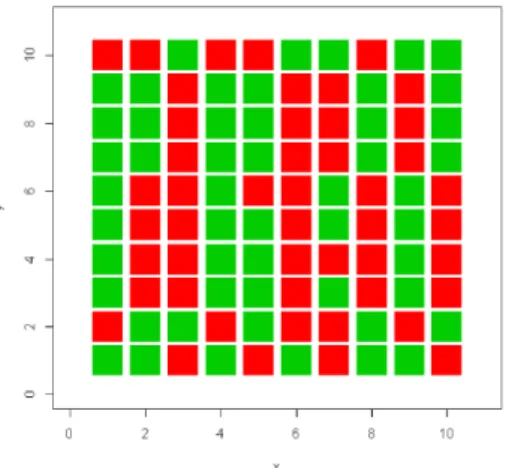
Figure 4.2. Chromatc matrix that corresponds to the matrix of total efects. Positve efects: green; negatve ef-fects :red. The nutrient y1, and the herbivores y4, y5 are the components that have a positve impact on a larger num-ber of species. The herbivores y3, y6are the components that have a negatve impact on a larger number of species
Figure 4.2 suggests that the causality in CAS is formed by a web of dynamic interdependencies (Hooker, 2011:885).
4.4 The Identification of Controlling Components in Ecosystems
In this secton, I will use data of the well known research project of Isle Royale (www.isleroyalewolf.org; Nelson, Peterson, and Vucetch, 2008). This project is the longest uninterrupted study of a predator–prey relatonship in the world.
The columns of the data, from left to right, are: the number of wolves (W), the number of moose (M), average temperature of January, and February (wtemp), average precipitaton of January, and February (wprecip), and average temperature of July, and September (stemp).
To apply the procedure to this data, the following script is used:
> library(MARSS) > library(mAr) > library(igraph) > #Data isleRoyal > royale.dat=(isleRoyal[1:53,c(2,3,4,10,6)]) > > #Obtaining MAR(1) > y=mAr.est(royale.dat,1,1)
>
> #The matrix of coefficients is matrix y$AHat > E=-ginv(y$AHat) # Total effects matrix
>
> #Obtaining total positive effects matrix > AS=E > n=1:5 > for (i in n) { + for (j in n) { + if (AS[i,j]<0) {AS[i,j]=0} + } + } > rownames(AS)=c('W','M','wtemp ','wprecip','stemp') > colnames(AS)=rownames(AS) > > #Network analysis > net.adjacency=AS > net= graph.adjacency(net.adjacency) > > #Desired transitivity > TR=transitivity(net, type="weighted") > round(TR,3)
[1] 0.667 NaN 0.667 1.000 1.000 The transitivity of the nodes
The output of the script is inserted in table 17.2.
Table 4.2. The transitvity values of the components of the data of Isle Royale W M wtemp wprecip stemp 0.667 NaN 0.667 1.000 1.000
To evaluate the results in table 17.2, I use the appreciaton of the project inserted in Nelson, Peterson, and Vucetch (2008). In page 108 of this paper it is stated the following:
- ‘Wolves seemed to have relatvely litle impact on moose abundance’, and they are the least important factor that afects short-term fuctuatons in moose abundance.
- ‘Climatc factors (such as summer heat and winter severity) are much more important’.
In table 17.2, only two climatc factors have values of transitvity equal to 1. One parameter is measured in summer (temperature), and the other in winter (precipitaton). Thus, the results in table 17.2 agree with the empirical evidence recorded in Nelson, Peterson, and Vucetch (2008:108).
4.5 Conclusive Remarks
The results obtained support the applicaton of the proposed procedure to identfy keystone species, and controlling components in ecosystems.
The discovery of the relaton between autocatalysis and total positve efects is conceptually, and theoretcally relevant. The relevance of the process of autocatalysis for the structure, and dynamics of ecosystems is here corroborated, and reinforced.
It is also shown that the aggregaton of several diferent tools, and concepts in new synthesis can give rise to new insights, and operatonal procedures, capable of solving relevant problems.
4.6 References, and Related Bibliography
Barbosa, S. M., 2012. mAr: Multvariate AutoRegressive analysis. R package version 1.1-2. htps://CRAN.R-projec-t.org/package=mAr
Barreto, L. S., 2011. From Trees to Forests. A Unified Theory. E-book. Costa de Caparica.
Barreto, L. S., 2016. Ecologia Teórica. Uma outra Explanação. III. Comunidade e Ecossistema. E-book. Costa de Ca-parica.
Barreto, L. S., in press. A Procedure to Identfy Keystone Species, and Controlling Components in Ecosystem. Sub-mited to Silia Lusitana in April, 2017.
Csárdi, G., and T. Nepusz, 2006. The igraph software package for complex network research. InterJournal, Complex
Systems, 1695. htp://igraph.org
Holmes, E., E. J. Ward, and K. Wills, 2012. MARSS: Multvariate Auto-Regressive State-Space Models for Analizing Time Series. The R Journal, 4(1):11-19.
Hooker, C., 2011. Introducton to Philosophy of Complex Systems. In Clif Hooker, Editor, Philosophy of Complex
Systems, Elsevier, pages 842-909.
Jain, S., and S. Krishna, 2001. Crashes, Recoveries, and ‘Core-Shifts’ in a Model of Evolving Networks. Proceedings of
the Natonal Academy of Sciences USA, 98:543-547.
Jain, S., and S. Krishna, 2002. Large Extnctons in an Evolutonary Model: The Role of Innovaton and Keystone Species. Proceedings of the Natonal Academy of Sciences USA, 99:2055-2060.
Jordán, F., 2009. Keystone species and food webs. Philos Trans R Soc Lond B Biol Sci., 364(1524): 1733–1741. doi: 10.1098/rstb.2008.0335
Jørgensen, S. E., (Main editor), 2009a. Ecosystem Ecology. Elsevier, Amsterdam.
Kolaczyk, E. D., and G. Csárdi, 2014. Statstcal Analysis of Network Data with R. Springer, Berlin.
Libralato, S., V. Christensenc, and D. Paulyc, 2006.A method for identfying keystone species in food web models.
Ecological Modelling, 195:153–171.´
Nelson, M. P., Rolf O. Peterson, and John A. Vucetch, 2008. The Isle Royale Wolf–Moose Project: Fifty Years of Challenge and Insight. The George Wright Forum, 25(2):98-113.
Ramsey, D., and C. Veltman, 2005. Predictng the efects of perturbatons on ecological communites: what can qualitatve models oferv. Journal of Animal Ecology, 74: 905–916. doi: 10.1111/j.1365-2656.2005.00986.x
Salas, A. K., and S. R. Borret, 2011. Evidence for the dominance of indirect efects in 50 trophic ecosystem networks. Ecological Modelling, 222 (2011): 1192–1204.
Scharler, U. M., 2009. Ecological Network Analysis, Ascendency. Em S. E. Jørgensen, Compilador principal,
Ecosystem Ecology. Elsevier, Amsterdam. Páginas 57-64.
Smith, C. et al, 2014. Report on identficaton of keystone species and processes across regional seas. Deliverable 6.1, DEVOTES Project. 105 pp + 1, Annex.
Tanner, J. E., T. P. Hughes, and J. H. Connell, 1994. Species coexistence, keystone species, and succession: a sensitvity analysis. Ecology, 75(8):2204-2219.
Ulanowicz, R.E., 1980. An hypothesis on the development of natural communites. J. theor. Biol. , 85: 223–245. Ulanowicz, R.E., 2004. Quanttatve methods for ecological network analysis. Computatonal Biology and Chemistry, 28:321 – 339.
Ulanowicz, R.E., 2009. Autocatalysis. Em S. E. Jørgensen, (Main editor), Ecosystem Ecology. Elsevier, Amsterdam. Pagess 41-43.
Zhao, L. et al., 2016. Weightng and indirect efects of identfy keystone species in food webs. Ecology Leters, 19:1033-1040.
5 Developmental, Structural, and Functional Sensitivities to Initial
Values
5.1 Introduction
With the growth, and spread of human populaton, the predicton of the response of populatons, communites, and ecosystems to anthropogenic impacts is an issue that must receive the atenton of ecology researchers.
It is our understanding that keystone species, and controlling factors are the extreme case of the sensitvity of the ecosystem to their components.
Thus, the transitvity of the biotc, and non living components of the ecosystem (e.g., tables 4.1, and 4.2) are a metric for the developmental, structural, and functonal sensitvites of the ecosystem to the perturbatons of each one of them, per se.
This conjecture also originates a tool to distnguish ecosystems that start in diferent points of the basin of atracton of a given fxed point. These ecosystems have diferent community matrices, and thus diferent MTPE, although they have a common fxed point.
To accomplish the scope of this chapter we considered three variants of the ecosystem described in the previous chapter. They are:
• The ecosystem without competton; • The ecosytem without mutualism;
• Only the interacton resource-consumer (trophic web)
To each one of these four ecosystems we applied SBCANAL. The results are exhibited in table 5.1
Table 5.1. Weighted values of the transitvity of the networks associated to the MTE of the four mentoned ecosystems. WO = without omissions; WC = without competton; WM = without mutualism; OT = only trophic interacton 1 2 3 4 5 6 7 8 9 10 WO 0,333 0,700 0,571 0,476 0,600 0,667 0,900 0,600 0,667 1,000 WC 0,444 0,467 0,600 0,600 0,600 0,600 0,667 1,000 0,833 1,000 WM 0.333 0.300 0.400 0.667 0.500 0.500 0.667 1.000 NaN 0.667 OT 0.476 0.600 0.476 0.800 0.800 0.524 0.667 0.800 0.667 0.833
The concepts in the ttle of this chapter have the meaning conferred to them in context of the analysis of ascendency. Thus, before we proceed we clarify this concept, and the associated network analysis.
5.2 Ascendency
The concepts, and indices presented in this secton were developed with the purpose of analyse networks including a sole interacton: the food web.
If the reader is familiar with the model for ecological succession proposed by Odum (Odum, and Barret, 2005:Table 8-1), consistent with the model of facilitaton, knows that in this concept the succession reveals directonality, this is, the development of the succession is characterized by the emergence of a predictable sequence of communites that evince a set of
atributes that have a fxed patern of change. Some of them are characterized in fgure 5.1. In the axis of tme occurs the sequence of communites.
+
Figure 5.1. Patern of the evoluton of some atributes of the communites, along the succession. The stages of the succession move along the axis of tme. To obtain these graphics in R, I adopted the scripts in Basic, displayed in Odum, and Odum (2000:257)
It is our understending that according to the concept of ecosystem development proposed by Jørgensen (2009a), and Jørgensen et al, (2007), this development has also directonality. In this concepton of ecosystem, directonality is a basic property of ecosystems. Ecosystems reveal also
openness, hierarchy, connectvity among their components, and complex dynamics. From these
propertes it is possible to obtain 10 atributes candidates to ecological laws (Jørgensen, 2009b:5, Table 1).
Directonality implies self-organizaton, and self-regulaton, this is, due only to internal processes of the system, emerge self-sustained order, and structure.
In fgure 5.2 we represent a system of four components, limited by a fronter. This is, there is the internal space of the system, and the external space where the system exists. The components interact through a loop of positve efects. The network of fgure 5.2 is also called a
autocatalytc cycle (ACC), positve feedback loop, loop of positve directed interacton. The mutualistc interacton between two species is a simple ACC. We can say that autocatalyse is a generalized form of mutualism.
Figure 5.2. Autocatalyse (black arrows), and centripetality (green arrows crossing the system fronter, atracted by its components), in a system with four compartments. Red arrows represent dissipaton of non usable materials or/and energy
The ACC gives origin to a spiral of growing benefts to the components of the cycle. It is the autocatalyse that provokes the emergence of directonality, and centripetality (atracton to the centre) in the ecosystem. Centripetality is the capacity of the system to atract resources, and free energy from the surroundings to its internal space, after they had crossed the system’s fronter. In fgure 1.1 we atempted to present a graphical syntheses of the causal chain triggered by autocatalyse. Autocatalyse promotes the increment of the organizaton of the ecosystem. The degree of organizaton is measured by ascendency, to be detailed later.
The archetype of the system studied by the analysis of ascendency is illustrated in fgure 5.3. A reifcaton of this archetype is exhibited in fgure 5.6.
Figure 5.3. Ecosystem formed by four compartments that can be biotc or non living. The other compartments can be, or not, related to the outer space as compartment 1