DOI 10.1007/s00442-016-3653-y
COMMUNITY ECOLOGY – ORIGINAL RESEARCH
Hierarchical spatial segregation of two Mediterranean vole
species: the role of patch‑network structure and matrix
composition
Ricardo Pita1,2 · Xavier Lambin3 · António Mira1 · Pedro Beja2,4
Received: 27 January 2016 / Accepted: 3 May 2016 / Published online: 11 May 2016 © Springer-Verlag Berlin Heidelberg 2016
tended to be the sole occupant of landscapes with high habitat amount but relatively low patch density (i.e., with a few large patches), and with a predominantly agricultural matrix, whereas landscapes with high patch density (i.e., many small patches) and low agricultural cover, tended to be occupied exclusively by the small Cabrera vole. The two species tended to co-occur in landscapes with inter-mediate patch-network and matrix characteristics, though their extents of occurrence were negatively correlated after controlling for environmental effects. In combination with our previous studies on the Cabrera-water vole sys-tem, these findings illustrated empirically the occurrence of hierarchical spatial segregation, ranging from within-patches to among-landscapes. Overall, our study suggests that recognizing the hierarchical nature of spatial segrega-tion patterns and their major environmental drivers should enhance our understanding of species coexistence in patchy environments.
Keywords Cabrera vole · Competition · Landscape
heterogeneity · Patchy environments · Species coexistence · Southern water vole
Introduction
Understanding the mechanisms facilitating the coexistence of potential competitors in patchy environments is a long-standing topic in ecology (Hanski 1983; Chesson 2000; Amarasekare 2003; Valladares et al. 2015). Most studies have addressed this problem by evaluating how species seg-regate along patch-level niche axes, such as food, micro-habitat or time of activity (Holt 2001; Jorgenson 2004; Leibold and McPeek 2006). However, it is possible that coexistence may also be facilitated by niche partitioning
Abstract According to ecological theory, the coexistence
of competitors in patchy environments may be facilitated by hierarchical spatial segregation along axes of environ-mental variation, but empirical evidence is limited. Cabrera and water voles show a metapopulation-like structure in Mediterranean farmland, where they are known to seg-regate along space, habitat, and time axes within habitat patches. Here, we assess whether segregation also occurs among and within landscapes, and how this is influenced by patch-network and matrix composition. We surveyed 75 landscapes, each covering 78 ha, where we mapped all habitat patches potentially suitable for Cabrera and water voles, and the area effectively occupied by each species (extent of occupancy). The relatively large water vole
Communicated by Janne Sundell.
Electronic supplementary material The online version of this article (doi:10.1007/s00442-016-3653-y) contains supplementary material, which is available to authorized users.
* Ricardo Pita
1 Unidade de Biologia da Conservação, CIBIO/InBio-Centro de Investigação em Biodiversidade e Recursos Genéticos, Universidade de Évora, Pólo de Évora, Núcleo da Mitra, Apartado 94, 7002-554 Évora, Portugal
2 CEABN/InBIO, Centro de Ecologia Aplicada “Professor Baeta Neves”, Instituto Superior de Agronomia, Universidade de Lisboa, Tapada da Ajuda, 1349-017 Lisboa, Portugal 3 School of Biological Sciences, University of Aberdeen,
Aberdeen AB24 2TZ, UK
4 EDP Biodiversity Chair, CIBIOI/InBIO-Centro de Investigação em Biodiversidade e Recursos Genéticos, Universidade do Porto, Campus Agrário de Vairão, Porto 4485-661, Vairão, Portugal
beyond local habitat patches, with, for instance, variation in patch-network structure and matrix composition contribut-ing to determine whether two competitors can coexist at the local and regional levels (Hanski and Ranta 1983; Yu et al.
2001; Nowakowski et al. 2013). Although this idea has been widely addressed theoretically, empirical investiga-tion of landscape-level niche partiinvestiga-tioning remains relatively scarce (Amarasekare 2003; Boeye et al. 2014).
In a system with two asymmetric competitors, the most extreme case of landscape-level segregation may occur when the dominant competitor occupies all landscapes meeting its requirements in terms of, for instance, patch-network and matrix characteristics, while the subordinate competitor is forced into landscapes unsuitable for the dominant competitor (Schippers et al. 2015). In this case, coexistence would only be possible at the regional scale, because the two competitors would be unable to share the same landscapes. At the other extreme, the two species may always be able to coexist at the landscape level, which is often judged to result from the interplay between species’ limiting factors, competitive and colonization abilities, and the spatial distribution of shared resources (Amarasekare and Nisbet 2001; Amarasekare 2003; Hanski 2008). A situ-ation intermediate between these two extremes may also occur, with some landscape features leading to occupa-tion by either only the dominant or only the subordinate competitor, and others favoring the coexistence of the two species. For instance, the subordinate competitor may be totally absent from landscapes that are optimal for the dominant competitor, but be able to coexist or even be the sole occupant in less favorable landscapes (Durant 1998). However, even in landscapes where both species coexist, the dominant may still influence the subordinate competi-tor by constraining its distribution or abundance at smaller spatial scales (Amarasekare 2003; Schippers et al. 2015). Overall, therefore, it is possible that segregation may occur over a hierarchy of scales depending on environmental cir-cumstances, with potential competitors using, for instance, different landscape types, different patch types within land-scapes where they coexist, and different space, time, and food resources within those patches that are used simul-taneously. At present, little information is available to test these ideas, probably because this would require detailed data on species distribution and co-occurrence patterns across landscapes with different properties (e.g., Yu et al.
2001; Richter-Boix et al. 2007; Schmidt et al. 2008), which are often costly to collect and difficult to replicate in natu-ral systems, particularly for vertebrate species.
In this study, we used a system of two vole species that share similar resources in Mediterranean farmland land-scapes, to evaluate whether segregation occurs at more than one spatial scale, and whether segregation at different scales is associated with particular environmental conditions. We
focused on two species of conservation concern (Palomo et al. 2007), the Cabrera vole (Microtus cabrerae) and the southern water vole (Arvicola sapidus, hereafter water vole), which in agricultural landscapes exhibit a metap-opulation-like spatial structure, occupying similar patches dominated by wet and tall herbaceous vegetation, imbed-ded within matrices of varying land use types (Pita et al.
2007, 2013). Previous studies have shown that Cabrera and water voles share much the same food preferences, graz-ing mostly on evergreen annual and perennial monocoty-ledons, such as grasses, sedges, and rushes (Soriguer and Amat, 1988; Román 2007; Rosário et al. 2008). However, the species tend to segregate at the patch-level, along axes of space, microhabitat, and time of activity (Pita et al.
2010, 2011a, b). In the case of time, for instance, there was some evidence that the dominant competitor (water vole) excludes the subordinate competitor (Cabrera vole) from its preferred time of activity (Pita et al. 2011b). Segrega-tion beyond the patch-scale has never been assessed, but this may occur, because each species is strongly affected by landscape features such as patch-network structure and matrix composition (Pita et al. 2007, 2013). Therefore, to test whether segregation occurs over a hierarchy of spatial scales, we examined the distribution and co-occurrence patterns of the two species across replicate landscapes with variable habitat amount, patch density, and matrix com-position, assessing: (1) whether the two species coexist in some landscapes but not in others; (2) how shared and exclusive use by each species are shaped by landscape fea-tures; and (3) whether the area used by each species within shared landscapes (extent of occurrence) is consistent with a negative impact of the dominant competitor on the subor-dinate competitor (Guillaumet and Leotard 2015). Results are used to discuss the implications of hierarchical spatial segregation for understanding the coexistence of potential competitors in fragmented landscapes.
Methods Study system
The study was conducted in south west Portugal (37°21′– 38°04′N, 08°51′–08°30′W, Fig. 1a), which is character-ized by Mediterranean climate with oceanic influence, with mean monthly temperatures about 16 °C, and aver-age annual rainfall around 650 mm, of which >80 % falls between October and March (wet season) (Pita et al. 2009; Beja et al. 2014). During our study, the mean monthly tem-perature ranged from 11.2 °C (wet season, 2007) to 21.0 °C (dry season, 2006), and mean monthly precipitation ranged from 28.1 mm (dry season, 2008) to 101.0 mm (wet sea-son, 2006) (Table SM1 in Supplementary information). The
region is mainly devoted to mixed annual crop–livestock farming (>65 % of the study area), while woody cover is restricted to a few woodlots (mean ± SE = 3.54 ± 0.34 ha) and hedges with planted trees (mainly pines and eucalyp-tus) delimiting irrigated fields (Pita et al. 2009; Beja et al.
2014). Semi-natural habitats occur in dunes, stream val-leys, and cork oak woodlands surrounding the farmed area. Despite the overall trend for agricultural intensification since the early 1990s, some areas have been abandoned or maintain extensive agriculture, resulting in many landscape types and ecological gradients that reflect different man-agement options (Pita et al. 2009; Beja et al. 2014).
Cabrera and water voles occur in the study area as spa-tially structured populations, and they are both largely restricted to of wet and tall (≈>30 cm) herbaceous vegeta-tion dominated by grasses, sedges, rushes, and reeds, typi-cally along small streams, temporary ponds, field margins, and road verges (Pita et al. 2007, 2013). Within habitat patches, individuals of both species tend to show strong
site-fidelity, with mean ± SE (range) home-range sizes of 946.3 ± 126.3 m2 (198.2–2600.2 m2) for the larger-sized
water vole, and 418.2 ± 56.3 m2 (39.3–1075.6 m2) for the
smaller-sized Cabrera vole (Pita et al. 2010).
Sampling design
The study was conducted between 2006 and 2008, and was based on 75 landscapes selected across the study area. Each landscape corresponded to a circular area with ≈78 ha, encompassing vole habitat patches and the surrounding matrix occupied by a variety of land uses. The mean ± SE (range) nearest neighbor distance between centers of land-scapes was 3.6 ± 0.07 km (2.5–5.8 km) (see Fig. 1b). Landscape size was set to be much larger than the area used by adult breeding voles (i.e., >800 times larger than their mean home-ranges; Román 2007; Pita et al. 2010), while allowing replication across the region, such that a wide range of landscape types could be sampled (as in Bennett
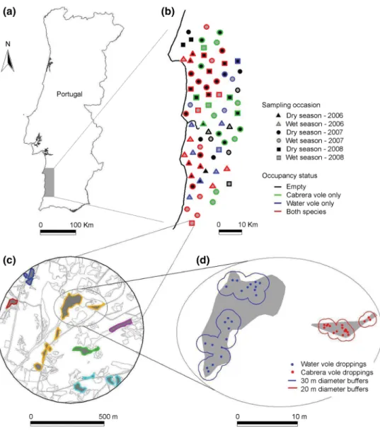
Fig. 1 a Map showing the loca-tion of the study area. b Distri-bution of surveyed landscapes with indication of the sampling occasion and occupancy status. c Example of habitat mapping in a landscape occupied by both species. Habitat polygons assigned to a single breeding patch as perceived by water voles, are identified by the same
color (see text for details). d Location of Cabrera and water vole droppings in suitable habitat (in gray), and respective 20- and 30- m diameter buffers used to estimate the extent of occupancy of each species (see text for details)
et al. 2006). A total of 20, 37, and 18 landscapes were sur-veyed in 2006, 2007, and 2008, respectively, with a total of 38, and 37 surveyed during the wet (October–March) and dry (April–September) seasons, respectively (Fig. 1b). In each landscape, a single snapshot survey was conducted to characterize the patch-network structure and matrix com-position, and to assess the (1) presence/absence of each species in the landscape, (2) and the extent of occupancy of each species within each landscape (see below).
Landscape variables
Suitable vole habitats were visually identified through sys-tematic field surveys and mapped from GPS recordings made along their borders, considering a minimum poly-gon area of 50 m2, and a minimum distance between
poly-gons (ground resolvable distance) of 5 m (Pita et al. 2013). Information was then incorporated in a geographical infor-mation system (GIS, ArcView 3.2, Redlands, CA, 1999). Patch networks were described by estimating the total area (ha) covered by suitable habitat for voles (hereafter referred to as habitat amount), and the number of potential breeding habitat patches (i.e., patches larger than the minimum area required for a breeding pair and respective progeny) per square km (hereafter referred to as patch density) (Fig. 1c).
Information on the minimum areas required by breeding pairs of Cabrera and water voles was unavailable, thus, we set the threshold based on the minimum home-range sizes for resident adults of each species observed in our study area (Pita et al. 2010), though excluding a few very small outliers. We considered that the minimum breeding patch for Cabrera voles corresponded to one or more habitat polygons distanced from each other by less than 50 m and covering a total habitat area of at least 250 m2. Breeding
habitat patches for water voles were estimated likewise, by setting the thresholds at 100 m and 500 m2, respectively.
After computing patch density estimates for the two spe-cies using these thresholds, we found that they were strongly correlated (Pearson’s r = 0.88, 95 %CI = 0.81– 0.92, P < 0.001). Therefore, in subsequent analysis for both Cabrera and water voles, we estimated patch densi-ties based on the threshold for the later species. This was a simplification, because the perceptual range of patchiness is species-specific (Swihart et al. 2003), but we believe it provides a reasonable basis to assess potential spatial seg-regation along patch density gradients (as in Basset 1995; Basset and de Angelis 2007). The rationale is that breed-ing area requirements of the smaller species are nested in those of the larger one (Basset and de Angelis 2007), and that occupied patches we treat as distinct units actu-ally function as independent local breeding populations for both species. This assumption would have been difficult to accept for water voles if we had defined patches based on
the threshold for the Cabrera vole. Some caution is needed when interpreting the results, however, as small patches potentially providing breeding areas for Cabrera voles (i.e., those between 250 and 500 m2) are necessarily overlooked.
These small patches represented only <5 % of the overall patch number, thus excluding them was unlikely to have had major impacts on our results.
The main types of land uses in the matrix expected to affect the species were also mapped in the GIS, based on high resolution (0.5 m/pixel) aerial photographs from 2005, and ground validation. These included the cover (ha) by agricultural fields (AGRO, land used for the production of cereals, vegetables, and other crops), extensive pastures (EPAST, semi-natural pastures, and fallows lightly grazed by cattle), improved pastures (IPAST, sown and irrigated pastures for cattle grazing), and the density (km/km2) of
irrigation structures (IRRIG, irrigation channels and drain-age ditches) (Pita et al. 2007, 2013; see Table 1 for sum-mary statistics).
Vole surveys
Cabrera and water vole surveys were based on systematic searches for their typical presence signs, in particular, fresh latrines or scattered droppings along runways, which are easily recognizable in the field (Fedriani et al. 2002; Pita et al. 2007, 2013). Searches at each landscape lasted in average (±SE, range) 4.1 ± 2.2 days (0.5–8 days), with more effort devoted to landscapes with larger amounts of potential habitat. Within each landscape, longer surveys were made in larger patches, with a minimum of about half an hour per patch. This sampling effort was judged to
Table 1 Summary statistics of landscape variables recorded per land-scape (n = 75) sampled for Cabrera and water voles in SW Portugal (2006–2008)
* Based on the perceptual ranges of the larger species, the water vole (see “Landscape variables” for details)
Set/variables Units Code Mean ± SE Range
Patch network Habitat amount ha HA 1.90 ± 0.26 0‒12.91 Breeding habitat patch density* *Patches/km2 PD 3.15 ± 0.23 0‒8.97 Matrix Cover agricultural land ha AGRIC 10.10 ± 1.68 0‒65.69 Cover extensive pastures ha EPAST 16.28 ± 1.85 0‒59.42 Cover intensive pastures ha IPAST 12.49 ± 2.13 0‒63.77 Density of irrigation structures km/km2 IRRIG 0.34 ± 0.11 0‒4.78
have minimized the likelihood of false negatives, as recent studies on the water vole suggest that occupancy may be detected in 80–100 % of cases during 30-min surveys, even in large patches (Fernández et al. 2016; Peralta et al. 2016). Considerable care was also taken to accurately distinguish the dropping of both species, which was mainly based on their sizes: length × width in mm of 4.8–9.6 × 1.8–3.2 in Cabrera voles versus 7.0–16.0 × 3.0–6.9 in water voles (Garrido-García and Soriguer 2014; Román 2014). Reli-ability in the identification of vole droppings was validated using molecular methods (Barbosa et al. 2013; Mira et al. unpublished data).
Sign surveys were always conducted in periods with no precipitation during at least the previous 2 days, to avoid flattening and wetting of feces. Searches consisted in scan-ning the whole surface of suitable habitats mapped, starting in preferred microhabitats (i.e., relatively taller and denser vegetation sites) and then expanding to other less suitable locations, so as to maximize the likelihood of detecting the target species (MacKenzie and Royle 2005; Peralta et al.
2016), which are often clustered on a particular portion of the patches. Searches often implied lifting the vegetation, though minimizing disturbance as much as possible. When vegetation density in one particular site was too high to walk through (e.g., bramble Rubus thickets), we searched around the edges enclosing that site. The locations of all vole droppings detected were recorded with a GPS with 5 m precision.
Surveys were used to estimate the occupancy of each landscape (hereafter landscape occupancy) consider-ing four possible categories: empty, occupied by either cabrera or water voles, and occupied by both species. We also estimated the extent of the area occupied by each spe-cies within each landscape (hereafter extent of occupancy), based on the spatial distribution of droppings. This was done by creating and merging buffers of 20 and 30 m diam-eters centered on each GPS location of Cabrera and water voles droppings, respectively (as in Pocock et al. 2003; see Fig. 1d). These buffer lengths were defined to provide a cir-cle with an area close to the mean home-range estimated in the study area for each species (Pita et al. 2010).
Data analysis
Multinomial logit (unordered) generalized mixed effect modeling (Multinomial GLMM) with Bayesian Markov chain Monte Carlo (MCMC) simulation was used to model the probability of landscape occupancy by each species alone and by both species together in relation to patch-network and matrix covariates, using empty landscapes as a baseline category. Landscapes without suitable vole habitats (i.e., patches dominated by wet and tall herbaceous vegetation) were dropped to avoid trivial results. We used
the maximal random intercept structure effects justified by our experimental design, so as to better control variation, increase the power of the analyses, and optimize generali-zation of the findings (e.g., Gillies et al. 2006; Barr et al.
2013). Therefore, we included in the random component four categorical variables reflecting potential effects of sampling year (three levels), sampling season (two levels), and spatial contagion in the distribution of Cabrera and water voles (four levels each, based on equal class intervals of the proportion of occupied landscapes in a 5-km buffer of each focal landscape). The buffer radius corresponded to the maximum dispersal distance recorded for the larger species, the water vole (Román 2007). Before analysis, covariates were scaled and log-transformed, to reduce the influence of extreme values and improve model conver-gence. Colinearity among all covariates was tested using variance inflation factors (VIF), and considering VIFs <2 as indicating acceptable levels of colinearity (Zuur et al.
2010).
In multinomial model building, we first assessed the effect of each covariate alone on landscape occupancy, and then selected as candidate those covariates which yielded deviance information criterion (DIC) values lower than that of the null model (including random effects only). This allowed reducing the number of possible covariates, and avoided the examination of candidate models with too many parameters relative to the number of observations (e.g., Kleinbaum et al. 1998). Candidate models includ-ing multiple covariates were then built usinclud-ing all possi-ble subsets of influential variapossi-bles. Due to limited sample size, only main effects were considered in model building. The best candidate model had the lowest DIC, but we also retained as equally supported all models at <5 DIC units from the best (ΔDIC). For each model, we estimated the 95 % credible intervals (CI) and pMCMC-values (signifi-cant pMCMC < 0.05) of each covariate. Model fit was esti-mated using pseudo-R2 (Johnson 2014). A similar
MCMC-GLMM modeling approach based on bivariate Gaussian distribution error was used to relate the extent of occu-pancy of each species to patch-network and matrix covari-ates. Empty landscapes were excluded from this analysis. Model posterior distributions were used to estimate the correlation between the two dependent variables; given as CorrMc,As= CovMc,As √VMc·VAs, where CovMc,As is the
covariance between the extents of occupancy of the Cabrera (Mc) and the water vole (As), and VMc and VAs represent
the respective variances (e.g., Hadfield 2010; Wilson et al.
2010). Significant correlations were determined by the 95 % credible intervals not overlapping with zero. For sim-plicity, we present, here, the results of the model yielding lowest DIC values in each set of analysis. Results regarding alternative models are presented in Supplementary material (Tables SM1–SM6).
GLMMs were run in the package ‘MCMCglmm’ ver-sion 2.19 (Hadfield 2010) using R 3.0.2 (R Develop-ment Core Team 2014), keeping >1000 posterior sam-ples (Hadfield 2012). Models were run until they reached acceptable low levels of first-order autocorrelation (gen-erally <0.08 for successive iterations) for both fixed and variance components (Plummer et al. 2006; Hadfield
2010), and until they reached convergence, as assessed visually using trace plots for both fixed effects and vari-ance components, and computationally using Geweke’s convergence diagnostic (Plummer et al. 2006). For mul-tinomial models, we used 1 × 10⁸ iterations, burn-in
size of 1 × 10⁵, and sampling every 5 × 10⁴ iterations,
whereas for Gaussian models, we used 3 × 10⁴
itera-tions, burn-in size of 3 × 10³, and thinning interval of
10 iterations. Prior specification in multinomial models followed Hadfield (2012), setting variance at one for all diagonal terms (variances) and 0.5 for all off-diagonal terms (covariances) in the residual structure. For ran-dom effects, we specified priors to have a variance equal to one, with a degree of belief (nu) equal to one. We screened multiple alternative priors and selected those producing the best trace plots of the variance compo-nents, though model results were largely insensitive to changes in the prior specification. For Gaussian models, we used default uninformative flat priors for the residual structure, while for the random component, we set the variance at one, and the nu at 0.002 (Gelman 2006; Had-field 2012). Adjusted pseudo-R2 were estimated with
‘MuMIn’ (Barton 2014).
Results
A total of 142.7 ha of suitable habitat for voles was found in 69 of the 75 landscapes surveyed, corresponding to ca. 3 % of the surveyed area. Overall, 184 patches > 500 m2
were identified in 68 landscapes, of which 51 and 42 % were occupied by Cabrera and water voles, respectively, and 18 % were occupied by both. Also, 17 small (<500 m2),
isolated (>100 m from the nearest patch) habitats were identified in 14 landscapes. From these, eight patches in seven landscapes could be considered as potentially pro-viding exclusive breeding patches for Cabrera voles (i.e., those between 250 and 500 m2). Presence signs of Cabrera
and water voles were found in three and one of these habi-tats, respectively, with no evidence for local co-occurrence. Overall, 62 landscapes were occupied by at least one spe-cies, of which 26 % were occupied exclusively by Cabrera voles, 17 % were occupied by water voles alone, and 46 % were occupied by both species (Fig. 1b).
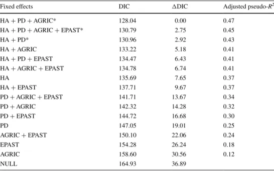
Colinearity among covariates was low (VIFs <2, see Supplementary material, Table SM2), and thus, they were all considered in the analyses. Multinomial MCMC-GLMM regressions with single covariates provided support for the influence of patch density, habitat amount, and proportional cover by agricultural land and extensive pastures on land-scape occupancy status (Supplementary material, Table SM3). These variables were used to build 16 candidates models, three of which were roughly equally supported (ΔDIC < 5; Table 2). Among these, the model including habitat amount, patch density, and cover by agricultural
Table 2 Candidate models to explain landscape occupancy by Cabrera and water voles, and their respective DIC values, ΔDIC, and adjusted pseudo-R2
* Indicates most supported models (ΔAIC ≤ 5). See Table 1 for variable codes
Fixed effects DIC ΔDIC Adjusted pseudo-R2
HA + PD + AGRIC* 128.04 0.00 0.47 HA + PD + AGRIC + EPAST* 130.79 2.75 0.45 HA + PD* 130.96 2.92 0.43 HA + AGRIC 133.22 5.18 0.41 HA + PD + EPAST 134.47 6.43 0.41 HA + AGRIC + EPAST 134.78 6.74 0.41 HA 135.69 7.65 0.37 HA + EPAST 137.71 9.67 0.37 PD + AGRIC + EPAST 141.71 13.67 0.34 PD + AGRIC 142.32 14.28 0.32 PD + EPAST 144.72 16.68 0.30 PD 147.05 19.01 0.25 AGRIC + EPAST 150.10 22.06 0.24 EPAST 154.28 26.24 0.18 AGRIC 158.60 30.56 0.12 NULL 164.93 36.89
land had the lowest DIC and an adjusted pseudo-R2 of 0.47
(Table 2). Results were largely consistent among the three best supported models (Supplementary material, Table SM4), indicating that landscape occupancy by water voles alone or by both vole species together was very significantly favored by higher amounts of habitat (pMCMC <0.001), while exclusive landscape occupancy by the Cabrera vole was significantly (pMCMC <0.05) favored by higher patch density. Also, landscapes with increased cover by agricul-tural land showed significantly higher probability of being occupied exclusively by water voles (Fig. 2a).
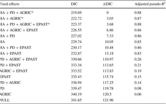
The mean ± SE (range) extent of occupancy per land-scape was 0.72 ± 0.11 ha (0–3.98) for Cabrera voles and 1.80 ± 0.26 ha (0–9.29) for water voles. Models including each single covariate alone provided support for the influ-ence of habitat amount, patch density, cover by agricul-tural land, and matrix cover by extensive pastures (Supple-mentary material, Table SM5). Three of the 16 candidate models built with these variables were equally supported (ΔDIC < 5; Table 3). The model including habitat amount, patch density, and cover by agricultural land yielded the
lowest DIC and an adjusted pseudo-R2 of 0.88 (Table 3).
This model indicated that the extents of occupancy of both Cabrera and water voles increased very significantly with the amount of habitat (Fig. 2b). For the Cabrera vole, there was also a significant positive effect of patch density and a significant negative effect of agriculture cover, while for water voles, there was a very significant positive effect of agricultural land cover (Fig. 2b). These results were con-sistent among the best supported models (Supplementary material, Table SM6). There was a significant negative correlation between the extents of occupancy of Cabrera and water voles after controlling for the effect of envi-ronmental variables (CorrMc,As; posterior mode = −0.39; 95 %CI −0.61 to −0.16).
Discussion
This study, together with previous research on the Cabrera-water vole system (Pita et al. 2010, 2011a, b), is consist-ent with the idea that segregation between the two species
Fig. 2 a Posterior estimates of model coefficients and 95 % CI for the first ranked multinomial MCMC-GLMM logit model relating landscape occupancy to habitat amount, patch density, and cover by agricultural land. Empty landscapes were the baseline category (loca-tion of the effects = 0) (see Supplementary material, Table SM3). b Posterior estimates of model coefficients and 95 % CI for the first
ranked bivariate Gaussian MCMC-GLMM models relating the extent of area occupied by Cabrera and water voles to habitat amount, patch density, and agricultural cover (see Supplementary material, Table SM6). Effective sample size was >1000 for all fixed effects in all models run. Asterisks indicate that coefficients are significantly dif-ferent from zero: *P < 0.05; **P < 0.001
probably occurs at more than one spatial scale, and that segregation at different scales is associated with particular environmental conditions. Specifically, we found that the two species coexisted in some landscapes but not in oth-ers, and that shared and exclusive use by each species were associated with total habitat amount, the density of habitat patches, and matrix composition. Also, we found evidence for a negative correlation between each species extent of occupancy within shared landscapes after controlling for patch-network and matrix variation. Overall, therefore, our study concurs to a growing body of evidence suggesting that segregation between competitors may occur at multi-ple hierarchical spatial scales, from within-patch to among-landscapes (e.g., Inouye 1999; Gilbert et al. 2008; Laporta and Sallum 2014), thus underlining the importance of con-sidering processes operating over a range of spatial scales to understand how competitors coexist in real landscapes (Whittaker et al. 2001; Kneitel and Chase 2004).
Vole segregation among landscapes
Segregation patterns of water and Cabrera voles among landscapes were partly consistent with the idea that the large and putatively dominant competitor tended to occupy all landscapes meeting its requirements in terms of patch-network and matrix characteristics, while the smaller and putative subordinate competitor seemed to be partly forced into landscapes unsuitable for the dominant competitor. This was supported by the observation that water voles tended to be the sole occupants of landscapes with large habitat patches (i.e., landscapes with high habitat amount but relatively low patch density) and high matrix cover by
agricultural land, which were shown previously to ben-efit this species (Pita et al. 2013). Because water voles are relatively large, large patches may provide conditions for a large number of individuals, and thus, reduce the prob-ability of local extinction (Pita et al. 2013; Sutherland et al.
2014). Agricultural land may be beneficial to water voles, because the wet margins that typically appear along irri-gated fields are likely to offer habitat and dispersal oppor-tunities across the dry farmland (Telfer et al. 2003; Cen-teno-Cuadros et al. 2011; Pita et al. 2013). Reasons for the absence of Cabrera voles in landscapes with these charac-teristics are uncertain, but this may result, to at least some extent, from competitive exclusion by water voles. In fact, previous studies have shown that the probability of patch occupancy by Cabrera voles increases with patch size (Pita et al. 2007), and so, they would be expected to occur in landscapes dominated by large patches, such as those used exclusively by water voles. It is noteworthy, therefore, that exclusive occupancy by Cabrera voles was associated with landscapes with many small patches (i.e., landscapes with high patch density), which were probably unsuitable for water voles, because most patches were too small for sus-taining local populations (Pita et al. 2013).
Although these observations provide support for compet-itive exclusion of Cabrera voles in some landscape types, we cannot rule out the possibility of the patterns observed resulting at least partly from independent and species-spe-cific responses to patch-network, matrix or other habitat characteristics. For instance, the negative association of Cabrera vole to landscapes with high amount of agricul-tural land may be related to reduced dispersal ability, and thus, reduced capacity to colonize empty habitat patches
Table 3 Candidate models to explain the extent of occupancy of Cabrera and water voles within landscapes, and their respective DIC values, ΔDIC, and adjusted pseudo-R2
* Indicates most supported models (ΔAIC ≤ 2). See Table 1 for variable codes
Fixed effects DIC ΔDIC Adjusted pseudo-R2
HA + PD + AGRIC* 219.69 0 0.88 HA + AGRIC* 222.72 3.03 0.87 HA + PD + AGRIC + EPAST* 223.37 3.68 0.88 HA + AGRIC + EPAST 226.55 6.86 0.86 HA + PD 227.02 7.33 0.86 HA 229.74 10.05 0.85 HA + PD + EPAST 230.17 10.48 0.86 HA + EPAST 232.87 13.18 0.83 PD + AGRIC + EPAST 330.66 110.97 0.26 PD + EPAST 333.34 113.65 0.21 AGRIC + EPAST 333.52 113.83 0.19 EPAST 335.43 115.74 0.15 PD + AGRIC 336.94 117.25 0.14 PD 339.47 119.78 0.08 AGRIC 340.19 120.5 0.06 NULL 341.65 121.96
(Pita et al. 2007), rather than a negative response to water voles per second. Elucidating this would require experi-mental studies, manipulating, for instance, the presence of water voles or the cues of its presence (e.g., droppings) in landscapes occupied by Cabrera voles, or the density and size of patches at the landscape scale (e.g., Ginger et al.
2003; Brunner et al. 2013). Future studies should also con-sider the role of other competitors and shared predators, as these have not been examined so far but they can strongly affect the interactions between potential competitors (e.g., Oliver et al. 2009).
Vole coexistence within landscapes
Although we found Cabrera and water vole segregation among some landscapes types, the two species actually co-occurred in most of the surveyed landscapes. This was in line with previous observations indicating that both species can coexist within the same patches (Pita et al. 2010, 2011a,
b), and suggest that coexistence may be further facilitated by some patch-network and matrix characteristics. Spe-cifically, we found that coexistence was most likely where the habitat amount was high, but where patch density was also much higher than in landscapes occupied exclusively by water voles, which may reflect landscapes with a diver-sity of large and small patches. In these landscapes, small patches unsuitable for water voles may serve as refuges for Cabrera voles, and they may provide sources of individu-als colonizing larger patches temporarily left vacant or only partly occupied by water voles. High patch density may also be related to small inter-patch distance, which may favor dispersal, and thus increase colonization ability by the Cabrera vole, which seems to have much lower disper-sal ranges than water voles (Pita et al. 2007, 2013). We also found that landscapes occupied by both Cabrera and water voles had an intermediate cover by agricultural land uses, in relation to those occupied solely by either species. This may be due to the contrasting response of the two species to this variable, with the colonization ability of Cabrera voles declining with increasing cover by agricultural land (Pita et al. 2007), and the opposite presumably occur-ring for water voles (Pita et al. 2013). Overall, therefore, it seemed that coexistence was favored in landscapes that were suboptimal for water voles (relatively small patches and intermediate cover by agricultural land), and that at the same time provided refuges (small patches) and dispersal opportunities (non-agricultural land, short inter-patch dis-tance) for Cabrera voles.
As for the segregation among landscapes, it was difficult to assess whether the observed patterns of within-landscape coexistence resulted from independent, species-specific responses to environmental factors, or whether it also involved some kind of competitive interference between
species. However, we found that the extent of occurrence of water and Cabrera voles within shared landscapes was negatively correlated after controlling for potentially con-founding environmental effects, which is compatible with a negative effect of the putative dominant on the putative subordinate competitor. These results suggest that in the absence of water voles and for constant environmental conditions, the area occupied by Cabrera voles would be larger than that observed in our study. This might be a con-sequence, for instance, of water voles displacing Cabrera voles from some suitable patches (i.e., segregation among patches), or by limiting the extent of occupancy of Cabrera voles in patches occupied by both species (i.e., within-patch segregation). Testing these hypotheses should be the subject of future research.
Implications for the coexistence of competitors
The coexistence of competitors occupying habitat patches in fragmented landscapes is generally interpreted as result-ing from the partitionresult-ing of resources at local scales (clas-sical niche-based mechanisms; e.g., Chase and Liebold
2003; Jorgenson 2004; Leibold and McPeek 2006), or from life-history tradeoffs, for instance, in competitive and colonization abilities (e.g., Amarasekare 2003; Hanski
1983, 2008). The observational studies carried out so far on the Cabrera-water vole system are insufficient to fully support or contradict either of these hypotheses, but they suggest that the mechanisms facilitating coexistence may be more complex than previously envisaged, because dif-ferent processes may operate simultaneously, though their relative importance may vary across spatial scales (Knei-tel and Chase 2004). On the one hand, our previous stud-ies suggest that coexistence within local patches may be facilitated by segregation along time and habitat axis (Pita et al. 2010, 2011a, b), which is consistent with niche-based mechanisms (Chase and Liebold 2003). However, the present study suggests that niche-based mechanisms may also operate at the landscape level, as segregation versus coexistence appeared to be influenced by species habitat preferences in terms of patch-network and matrix characteristics (Morris 1987; Yu et al. 2001; Westphal et al. 2006). On the other hand, however, our study also pointed out the possibility of life-history trade-offs facili-tating coexistence within landscapes, with the smaller spe-cies offsetting its lower competitive ability by occupying small habitat patches that are hardly occupied by the larger competitor, thereby enabling a fugitive-like coexistence (Amarasekare 2003; Hanski 1983, 2008). Whatever the mechanism or combination of mechanisms at play here, our results support the need to account for the hierarchi-cal nature of species spatial segregation patterns to gener-ate robust hypotheses about the processes that allow their
coexistence (Kneitel and Chase 2004; Szabó and Meszéna
2006; Kneitel 2012). In particular, because habitat patch-network structure and matrix composition are key land-scape properties in determining scales at which segrega-tion takes place, we suggest that spatial heterogeneity at the landscape scale should be routinely considered in both theoretical and empirical studies aiming to understand spe-cies coexistence in patchy environments (e.g., Gilbert et al.
2008; Biswas and Wagner 2012; László and Tóthmérész
2013) This, in turn, will provide invaluable information to support inferences on possible mechanisms facilitat-ing coexistence across multiple scales, and for improvfacilitat-ing conservation actions targeting multiple interacting species (Poiani et al. 2000; Tscharntke et al. 2012).
Acknowledgments This study was financed by FEDER funds through the Programa Operacional Factores de Competitividade— COMPETE, and National funds through the Portuguese Foundation for Science and Technology—FCT, within the scope of the projects PERSIST (PTDC/BIA-BEC/105110/2008), NETPERSIST (PTDC/ AAG-MAA/3227/2012), and MateFrag (PTDC/BIA-BIC/6582/2014). RP was supported by the FCT grant SFRH/BPD/73478/2010 and SFRH/BPD/109235/2015. PB was supported by EDP Biodiversity Chair. We thank Rita Brito and Marta Duarte for help during field work. We thank Chris Sutherland, Douglas Morris, William Morgan, and Richard Hassall for critical reviews of early versions of the paper. We also thank two anonymous reviewers for helpful comments to improve the paper.
Authors contribution statement RP, AM, PB conceived and designed the experiments. RP performed the experiments. RP, XL, AM, and PB analyzed the data. RP, XL, AM and PB wrote the manuscript.
References
Amarasekare P (2003) Competitive coexistence in spatially structured environments: a synthesis. Ecol Lett 6:1109–1122
Amarasekare P, Nisbet R (2001) Spatial heterogeneity, source-sink dynamics and the local coexistence of competing species. Am Nat 158:572–584
Barbosa S, Pauperio J, Searle JB, Alves PC (2013) Genetic identifi-cation of Iberian rodent species using both mitochondrial and nuclear loci: application to noninvasive sampling. Mol Ecol Resour 13:43–56
Barr DJ, Levy R, Scheepers C, Tily HJ (2013) Random effects struc-ture for confirmatory hypothesis testing: keep it maximal. J Mem Lang 68:255–278
Barton K (2014) Package ‘MuMIn’. Model selection and model aver-aging based on information criteria. R package version 1.10.5 Available at: http://cran.r-project.org/web/packages/MuMIn/ MuMIn.pdf
Basset A (1995) Body size-related coexistence: an approach through allometric constraints on home-range use. Ecology 76:1027–1035
Basset A, De Angelis DL (2007) Body size mediated coexist-ence of consumers competing for resource in space. Oikos 116:1363–1377
Beja P, Schindler S, Santana J, Porto M, Morgado R, Moreira F, Pita R, Mira A, Reino L (2014) Predators and livestock reduce bird
nest survival in intensive Mediterranean farmland. Eur J Wildl Res 60:249–258
Bennett AF, Radford JQ, Haslem A (2006) Properties of land mosa-ics: implications for nature conservation in agricultural environ-ments. Biol Conserv 133:250–264
Biswas SR, Wagner HH (2012) Landscape contrast: a solution to hid-den assumptions in the metacommunity concept? Landscape Ecol 27:621–631
Boeye J, Kubisch A, Bonte D (2014) Habitat structure mediates spatial segregation and therefore coexistence. Landscape Ecol 29:593–604 Brunner JL, Duerr S, Keesing F, Killilea M, Vuong H, Ostfeld RS
(2013) An experimental test of competition among mice, chip-munks, and squirrels in deciduous forest fragments. PLoS One 8:e66798
Centeno-Cuadros A, Román J, Delibes M, Godoy JA (2011) Prison-ers in their habitat? Generalist dispPrison-ersal by habitat specialists: a case study in southern water vole (Arvicola sapidus). PLoS One 6:e24613
Chase JM, Liebold MA (2003) Ecological niches: linking classical and contemporary approaches. University of Chicago Press, Chicago Chesson P (2000) General theory of competitive coexistence in
spa-tially-varying environments. Theor Popul Biol 58:211–237 Durant SM (1998) Competition refuges and coexistence: and example
from Serengeti carnivores. J Anim Ecol 67:370–386
Fedriani JM, Delibes M, Ferreras P, Román J (2002) Local and land-scape habitat determinants of water vole distribution in a patchy Mediterranean environment. Ecoscience 9:12–19
Fernández N, Román J, Delibes M (2016) Variability in primary pro-ductivity determines metapopulation dynamics. P R Soc B Biol Sci 283:20152998
Garrido-García JA, Soriguer RC (2014) Topillo de Cabrera Iberomys
cabrerae (Thomas, 1906) In: Calzada J, Clavero M, Fernández A (eds) Guía virtual de los indicios de los mamíferos de la Penín-sula Ibérica, Islas Baleares y Canarias. Sociedad Española para la Conservación y Estudio de los Mamíferos (SECEM). http:// www.secem.es/guiadeindiciosmamiferos/
Gelman A (2006) Prior distributions for variance parameters in hierar-chical models. Bayesian Anal 1:515–533
Gilbert B, Srivastava DS, Kirby KR (2008) Niche partitioning at mul-tiple scales facilitates coexistence among mosquito larvae. Oikos 117:944–950
Gillies CS, Hebblewhite M, Nielsen SE, Krawchuk MA, Aldridge CL, Frair JL, Saher DJ, Stevens CE, Jerde CL (2006) Application of random effects to the study of resource selection by animals. J Anim Ecol 75:887–898
Ginger SM, Hellgren EC, Kasparian MA, Levesque LP, Engle DM, Leslie DM Jr (2003) Niche shift by Virgina opossum follow-ing reduction of a putative competitor, the raccoon. J Mammal 84:1279–1291
Guillaumet A, Leotard G (2015) Annoying neighbors: multi-scale dis-tribution determinants of two sympatric sibling species of birds. Curr Zool 61:10–22
Hadfield JD (2010) MCMC methods for multi-response generalized linear mixed models: the MCMCglmm R package. J Stat Softw 33:1–22
Hadfield JD (2012) MCMCglmm Course Notes. Available online at:
http://cran.r-project.org/web/packages/MCMCglmm/vignettes/ CourseNotes.pdf
Hanski I (1983) Coexistence of competitors in patchy environments. Ecology 64:493–500
Hanski I (2008) Spatial patterns of coexistence of competing species in patchy habitat. Theor Ecol 1:29–43
Hanski I, Ranta E (1983) Coexistence in a patchy environment: three species of Daphnia in rock pools. J Anim Ecol 52:263–280 Holt RD (2001) Species coexistence. Encycl Biodiv 5:413–426
Inouye BD (1999) Integrating nested spatial scales: implications for the coexistence of competitors on a patchy resource. J Anim Ecol 68:150–162
Johnson PCD (2014) Extension of Nakagawa & Schielzeth’s R2
GLMM to
random slopes models. Method Ecol Evol 5: 44–946
Jorgenson EE (2004) Small mammal use of microhabitat reviewed. J. Mamm 85:531–539
Kleinbaum DG, Kupper LL, Muller KE, Nizam A (1998) Applied regression analysis and other multivariate models. Duxbury Press, California
Kneitel JM (2012) Are trade-offs among species’ ecological interac-tions scale dependent? A test using pitcher-plant inquiline spe-cies. PLoS One 7:e41809
Kneitel JM, Chase JM (2004) Trade-offs in community ecology: link-ing spatial scales and species coexistence. Ecol Lett 7:69–80 Laporta GZ, Sallum AAM (2014) Coexistence mechanisms at
multi-ple scales in mosquito assemblages. BMC Ecol 14:30
László Z, Tóthmérész B (2013) Landscape and local effects on mul-tiparasitoid coexistence. Insect Cons Divers 6:354–364
Leibold MA, McPeek MA (2006) Coexistence of the niche and neutral perspectives in community ecology. Ecology 87:1399–1410
MacKenzie DI, Royle JA (2005) Designing efficient occupancy stud-ies: general advice and allocating survey effort. J Appl Ecol 42:1105–1114
Morris DW (1987) Ecological scale of habitat use. Ecology 68:362–369
Nowakowski AJ, Hyslop NL, Watling JI, Donnelly MA (2013) Matrix type alters structure of aquatic vertebrate assemblages in cypress domes. Biodivers Conserv 22:497–511
Oliver M, Luque-Larena JJ, Lambin X (2009) Do rabbits eat voles? Apparent competition, habitat heterogeneity and large-scale coexistence under mink predation. Ecol Lett 12:1201–1209 Palomo LJ, Gisbert J, Blanco JC (2007) Atlas y Libro Rojo de los
Mamíferos Terrestres de España. Dirección General de Conser-vación de la, Naturaleza-SECEM-SECEMU
Peralta D, Leitão I, Ferreira A, Mira A, Beja P, Pita R (2016) Factors affecting southern water vole (Arvicolas sapidus) detection and occupancy probabilities in Mediterranean farmland. Mamm Biol 81:123–129
Pita R, Beja P, Mira A (2007) Spatial population structure of the Cabrera vole in Mediterranean farmland: the relative role of patch and matrix effects. Biol Conserv 134:383–392
Pita R, Mira A, Moreira F, Morgado R, Beja P (2009) Influence of landscape characteristics on carnivore diversity and abundance in Mediterranean farmland. Agric Ecosyst Environ 132:57–65 Pita R, Mira A, Beja P (2010) Spatial segregation of two vole species
(Arvicola sapidus and Microtus cabrerae) within habitat patches in a highly fragmented farmland landscape. Eur J Wildlife Res 56:651–662
Pita R, Mira A, Beja P (2011a) Assessing habitat differentiation between coexisting species: the role of spatial scale. Acta Oecol 37:124–132
Pita R, Mira A, Beja P (2011b) Circadian activity rhythms in relation to season, sex, and interspecific interactions in two Mediterra-nean voles. Anim Behav 81:1023–1030
Pita R, Mira A, Beja P (2013) Influence of land mosaic composi-tion and structure on patchy populacomposi-tions: the case of the water vole (Arvicola sapidus) in Mediterranean farmland. PLoS One 8(7):e69976
Plummer M, Best N, Cowles K, Vines K (2006) CODA: convergence diagnosis and output analysis for MCMC. R News 6:7–11 Pocock MJO, White PVL, McClean CJ, Searle JB (2003) The use
of accessibility in defining sub-groups of small mammals from point sampled data. Comput Environ Urban syst 27:71–83
Poiani KA, Richter BD, Anderson MG, Richter HE (2000) Biodiver-sity conservation at multiple scales: functional sites, landscapes, and networks. Bioscience 50:133–146
R Development Core Team. (2014) R: a language and environment for statistical computing, 3.0.2. R Foundation for Statistical Computing, Vienna, Austria
Richter-Boix A, Llorente GA, Montori A (2007) Structure and dynamics of an amphibian metacommunity in two regions. J Anim Ecol 76:607–618
Román J (2007) Historia natural de la rata de agua (Arvicola sapidus) en Doñana. PhD dissertation, Facultad de Ciencias, Universidad Autonoma de Madrid
Román J (2014) Rata de agua Arvicola sapidus Miller, 1908. In: Calzada J, Clavero M, Fernández A. (eds). Guía virtual de los indicios de los mamíferos de la Península Ibérica, Islas Baleares y Canarias. Sociedad Española para la Conservación y Estudio de los Mamíferos (SECEM). http://www.secem.es/ guiadeindiciosmamiferos/
Rosário IT, Cardoso PE, Mathias ML (2008) Is habitat selection by the Cabrera vole (Microtus cabrerae) related to food prefer-ences? Mamm Biol 73:423–429
Schippers P, Hemerik L, Baveco JM, Verboom J (2015) Rapid diver-sity loss of competing animal species in well-connected land-scapes. PLoS One 10(7):e0132383
Schmidt MH, Thies C, Nentwig W, Tscharntke T (2008) Contrasting responses of arable spiders to the landscape matrix at different spatial scales. J Biogeogr 35:157–166
Soriguer RC, Amat JA (1988) Feeding of Cabrera vole in west-central Spain. Acta Theriol 33:589–593
Sutherland CS, Elston DA, Lambin X (2014) A demographic, spa-tially explicit patch occupancy model of metapopulation dynam-ics and persistence. Ecology 95:3149–3160
Swihart RK, Atwood TC, Goheen JR, Scheiman DM, Munroe KE, Gehring TM (2003) Patch occupancy of North American mam-mals: is patchiness in the eye of the beholder? J Biogeogr 30:1259–1279
Szabó P, Meszéna G (2006) Spatial ecological hierarchies: coexist-ence on heterogeneous landscapes via scale niche diversification. Ecosystems 9:1009–1016
Telfer S, Piertney SB, Dallas JF, Stewart WA, Marshall F, Gow JL, Lambin X (2003) Parentage assignment detects frequent and large-scale dispersal in water voles. Mol Ecol 12:1939–1949 Tscharntke T, Tylianakis JM, Rand TA, Didham RK, Fahrig L, Batáry
P, Bengtsson J, Clough Y, Crist TO, Dormann CF, Ewers RM, Fründ J, Holt RD, Holzschuh A, Klein AM, Kleijn D, Kremen C, Landis DA, Laurance W, Lindenmayer D, Scherber C, Sodhi N, Steffan-Dewenter I, Thies C, van der Putten WH, Westphal C (2012) Landscape moderation of biodiversity patterns and pro-cesses—eight hypotheses. Biol Rev 87:661–685
Valladares F, Bastias CC, Godoy O, Granda E, Escudero A (2015) Species coexistence in a changing world. Front Plant Sci 6:866 Westphal C, Steffan-Dewenter I, Tscharntke T (2006) Bumblebees
experience landscapes at different spatial scales: possible impli-cations for coexistence. Oecologia 149:289–300
Whittaker RJ, Willis KJ, Field R (2001) Scale and species richness: towards a general, hierarchical theory of species diversity. J Bio-geogr 28:453–470
Wilson AJ, Réale D, Clements MN, Morrissey MM, Postma E, Wall-ing CA, Kruuk LEB, Nussey DH (2010) An ecologist’s guide to the animal model. J Anim Ecol 79:13–26
Yu DW, Wilson HB, Pierce NE (2001) An empirical model of spe-cies coexistence in a spatially structured environment. Ecology 82:1761–1771
Zuur AF, Leno EN, Elphic CS (2010) A protocol for data exploration to avoid common statistical problems. Method Ecol Evol 1:3–14