DOI: ISSN: Abstract — This article was motivated from a practical work
on modeling and control of a time-delayed thermal airflow process using adaptive techniques. The work was divided into two parts: (I) the modeling of the process using system identification methods, with main concerns to the numerical robustness of the identification, and (II) the digital control of the process using adaptive self-tuning control, with main concerns to the adaptation of the controller to changes in the process dynamics. This article presents the first part of the work. The thermal airflow system was represented by an ARMAX model, whose parameters were identified using the Recursive Least Squares method, based on two approaches: the Matrix Inversion Lemma, and the Bierman’s UD Factorization. The results obtained show that the last approach has greater numerical robustness and is more suitable for applications of adaptive control – the second part of the work, described in a separate article.
Index Terms — least squares, parameter estimation, recursive identification, system identification.
I. INTRODUCTION
Many problems on the design of automatic controllers for dynamic systems involve the determination of a suitable mathematical model for the system to be controlled. For digital control applications, a discrete-time model can be obtained either from the discretization of an available continuous-time model or from the direct determination of a discrete model by means of system identification or parameter estimation methods. Identification means the estimation of the parameters of a given discrete-time model, and can be implemented by either off-line (batch) or on-line (recursive) calculations. In the off-line identification, a set of input-output values (observations) from the system is measured along a suitable period of time, and then used as a whole data set in a batch calculation to estimate the parameters of a given model structure. In the on-line
identification, also known as real-time identification, the
S. A. A. Viana is a Senior Member of the IEEE – The Institute of Electrical and Electronics Engineers. He is currently with the Ferrous Automation Engineering Department of VALE, Belo Horizonte, MG, Brazil (e-mail: sidney.viana@vale.com).
model parameters are continuously estimated in a recursive fashion, by which the results computed at the previous sample time are used to compute the results for the current sample time. Recursive identification is particularly advantageous to track eventual changes on the system parameters, allowing an adaptive tuning of digital controllers. Mathematically, parameter identification is set of mathematical computations that intends to determine, under a certain optimality criterion, the values of model parameters that better match the input-output observations from the system. Recursive identification has fundamental importance in adaptive control, by which the controller parameters are automatically adjusted due to changes in the process parameters, provided that these changes are tracked by on-line identification. An interesting review of system identification methods can be found in [3].
This article describes the identification of an ARMAX (Auto-Regressive Moving Average with Exogenous Input) model for a thermal airflow system with time-delay. The identification was performed with the Least Squares method, based on two approaches: the Matrix Inversion Lemma [4][6][12], and the Bierman’s UD Factorization [4], with a comparison of the effectiveness of the two implementations.
The article is organized as follows: Section II describes the mathematical formulation of the Least Squares method in its non-recursive (off-line) and recursive (on-line) forms; Section III cares about the generation of suitable input signals for the system to be identified, in order to meet the requirement of persistent excitation. Section IV presents the model structure chosen for the process, and the results of the model identification using the Least Squares method. Finally, Section V summarizes the conclusions about this first part of the work, and its relationship with the second part.
II. THE LEAST SQUARES METHOD FOR SYSTEM IDENTIFICATION
A. Non-Recursive Form
The mathematical formulation of the Least Squares method was originally developed by Karl Friedrich Gauss for a problem of estimating the orbit of the Ceres asteroid [7]. Later, the method was extended to other kinds of estimation
Control of a Thermal Airflow Process with Time-Delay -
Part I: System Identification
Sidney A. A. Viana
problems.
For purposes of system identification, let us consider a simple ARX (Auto-Regressive with Exogenous Input) model: a a b b a b n n n n k n j j j n j j j k k z a z a z a z b z b z b b z z a z b z z A z B z z U z Y z G
2 2 1 1 2 2 1 1 0 1 0 1 1 1 1 ) ( ) ( ) ( ) ( ) ( (1)Fig. 1. Block diagram of an ARX model.
The discrete-time delay exponent k is a positive integer (k = 1, 2, 3, …), and its value depends on the sampling period T of the model. Without lack of generality, we can set k = 1. Cases in which k >1 can be considered similarly, increasing the order of the polynomial B(z–1) by k –1 and assuming the first k–1 coefficients bj are identically null. From the inverse
Z transform of Y(z) in (1), with k =1, the system output y(k) at the discrete time t = kT is:
) 1 ( ) 2 ( ) 1 ( ) ( ) 2 ( ) 1 ( ) ( 0 1 0 2 1 b a n n k u b k u b k u b n k y a k y a k y a k y a (2a)
Similarly, the system output for past discrete times
T N k T k T k t( 1) ,( 2) ,,( ) are: ) 2 ( ) 3 ( ) 2 ( ) 1 ( ) 3 ( ) 2 ( ) 1 ( 0 1 0 2 1 b a n n k u b k u b k u b n k y a k y a k y a k y a (2b) ) 1 ( ) 2 ( ) 1 ( ) ( ) 2 ( ) 1 ( ) ( 0 1 0 2 1 N n k u b N k u b N k u b N n k y a N k y a N k y a N k y b a na (2c)
The number of observations N must provide a sufficient number of equations to determine all the na+nb+1 unknown
parameters aj and bj, that is:
b a b a n N n n n N 1 1 (3)
Equations (2a) to (2c) can be written in matrix form as: ΦΘ
Y (4)
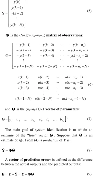
where Y is the (N+1)1 vector of outputs:
) ( ) 2 ( ) 1 ( ) ( N k y k y k y k y Y (5)
Φ
is the (N+1)(na+nb+1) matrix of observations: ) ( ) 2 ( ) 1 ( ) 2 ( ) 4 ( ) 3 ( ) 1 ( ) 3 ( ) 2 ( ) ( ) 2 ( ) 1 ( N n k y N k y N k y n k y k y k y n k y k y k y n k y k y k y a a a a Φ ) 1 ( ) 2 ( ) 1 ( ) 3 ( ) 4 ( ) 3 ( ) 2 ( ) 3 ( ) 2 ( ) 1 ( ) 2 ( ) 1 ( N n k u N k u N k u n k u k u k u n k u k u k u n k u k u k u b b b b (6)
and Θ is the (na+nb+1)1 vector of parameters:
T 1 0 2 1 a ana b b bnb a Θ (7)The main goal of system identification is to obtain an estimate of the “true” vector Θ. Suppose that Θˆ is an estimate of Θ. From (4), a prediction of Y is:
Θ Φ
Yˆ ˆ (8)
A vector of prediction errors is defined as the difference between the actual outputs and the predicted outputs:
Θ Φ Y Y Y E ˆ ˆ (9)
Ideally, if the estimate Θˆ is identically equal to the actual parameters vector Θ, the prediction errors vector E will be null. Therefore, the best estimate Θˆ is the one that minimizes the estimation errors E. Since the elements of E can assume either positive or negative values (and null value as well), we consider to minimize the sum of squares of the elements of E, leading to the following cost function:
Y
Φ
Θ
Y
Φ
Θ
E
E
E
2
T
ˆ
T
ˆ
J
(10)The minimization of the quadratic cost function (10) is the optimality criterion for the Least Squares method. The estimate Θˆ that minimizes J is obtained from:
0 ˆ 2 2 ˆ ΦTY ΦTΦΘ Θ d dJ (11)
Since ΦTΦ is non-negative definite, J is minimized for:
y(k) u(k)
DOI: ISSN:
Φ Φ
Φ YΘˆ T 1 T (12)
Equation (12) is called the Least Squares estimate of Θ. It only exists if ΦTΦ is non-singular, and then invertible. A
necessary condition for this is that the system is persistent excited, so that ΦTΦ does not have common lines. A formal
definition of persistent excitation is given in [11]. The matrix
ΦTΦ
1ΦT is called the pseudo-inverse ofΦ
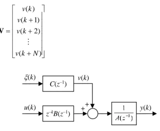
[4][6] [9][10].In practical applications, physical system usually involves a stochastic disturbance v(k), and the more generic ARMAX model shown in Fig. 2 should be used instead of the ARX model. The ARMAX model considers that the output y(k) is a result from the process input u(k) and a disturbance v(k), leading to a more accurate model than an ARX model. By this way, equation (4) is modified to:
V ΦΘ
Y (13)
Where V is the (N+1)1 vector of disturbances:
) ( ) 2 ( ) 1 ( ) ( N k v k v k v k v V (14)
Fig. 2. Block diagram of an ARMAX model.
Multiplying (13) by the pseudo-inverse
ΦTΦ
1ΦTand using (12), we obtain:
Φ Φ
Φ V ΘΘˆ T 1 T (15)
This means that estimate Θˆmay be biased, with standard deviation given by the following expected value:
ΦTΦ1ΦTV
E (16)
When the disturbance v(k) is an uncorrelated stochastic signal with null average, that is, a discrete white noise v(k) = (k), the expected value (16) will be null, and the estimate Θˆ will be unbiased. Otherwise, when the disturbance v(k) is a colored noise: ) ( ) 2 ( ) 1 ( ) ( ) ( 1 ) ( ) ( ) ( ) ( 2 1 2 2 1 1 1 1 c n n n n k c k c k c k k v z c z c z c z C k z C k v c c c
(17) then the estimate Θˆ given by (12) for an ARX model will be biased, unless the disturbance v(k) is included in the model. Therefore, to account for a stochastic disturbance in the system being identified, the ARMAX model must be used. The disturbance v(k) is assumed a white noise (k) filtered by polynomial C(z–1), whose coefficients are included in the extended parameters vector:
T 2 1 1 0 2 1 a ana b b bnb c c cnc a Θ (18) and the identification is referred as Extended Least Squares(ELS) [3].
B. Recursive Form
For purposes of adaptive control, the process parameters must be identified at each sampling interval, so that any change in those parameters can be tracked and used do adjust the controller parameters. This allows the controller to adapt to changes in the process dynamics. In this sense, the batch solution given by equation (12) is completely unpractical, since as the number of equations N increases, the dimensions of Y and
Φ
will also increase, causing computing overload in the digital computer that implements the identification and the control. It’s necessary that the previous parameters estimateΘ
ˆ
(
N
1
)
Θ
ˆ
N1 can be used to compute theestimate
Θ
ˆ
(
N
)
Θ
ˆ
N for the current time k = N. This is the key idea behind the recursive form of the Least Squares method.C. Recursive Least Squares with the Matrix Inversion Lemma
Recall the non-recursive formulation of the Least Squares given by equations (4) to (6). At the current time k = N, a new observation N is added to the observations matrix
Φ
, and anew element yN is added to the vector of outputs Y, that is:
N N N N N N y 1 1 ; Y Y Φ Φ (19) where:
1 2 1 3 2 1 b a N N N n n N N N N N u u u y y y y (20)Defining the covariance matrix P as:
T
1 Φ Φ
P (21)
from (12), the parameters estimate
Θˆ
Nfor all N observations at the sample time k = N is given by:N N N N P Φ Y Θˆ T (22) v(k) (k) u(k) + + C(z–1) y(k) z–kB(z–1)
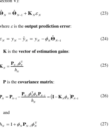
Using the Matrix Inversion Lemma [4][6][12], equation (22) can be modified to the following recursive form (see Section V): N N N N
Θ
K
Θ
ˆ
ˆ
1
(23)where is the output prediction error:
1
ˆ
ˆ
N N N N N Ny
y
y
Θ
(24)K is the vector of estimation gains:
N N N N h T 1
P K (25)P is the covariance matrix:
1 1 T 1 1 N N N N N N N N N N h I K P P P P P
(26) and T 1 1 N N N N h
P
(27)Equation (23) means that the parameters estimate is updated at each sampling time as:
Error Prediction Gain Estimate Previous Estimate Current (28)
Therefore, as the estimation proceeds and converges to the “true” parameters in Θ, the prediction error tends to zero, being an indicator of the convergence of the identification. The covariance matrix P is also indicative of the convergence. Since the magnitude of the elements in the main diagonal of P are related to the variances of the corresponding elements in the parameters estimate Θˆ , a small element pjj (low variance) in P means that the
corresponding parameter j is a good estimate. For practical
implementation, when there is no good guess about the actual values of the parameters in Θ, the diagonal elements in P can be set to high values (high initial variances). As the estimation proceeds, the updates in P by equation (24) will reduce the magnitudes of its diagonal elements, and the elements of the gain vector K tend to zero as the number of observations increases and the estimates converge. Therefore, by avoiding the diagonal elements in P to become overmuch low, the prediction error will provide a continuous correction of the parameters estimate Θˆ to its “true” value Θ , allowing to track eventual changes in Θ. This can be done by periodically resetting the covariance matrix P with high diagonal values.
A more efficient way to avoid the diagonal elements in P to decrease to zero is the use of a forgetting factor . It’s a factor between 0 and 1, set lightly small to 1, with the aim to progressively eliminate the influence of past observations on the updates of P, which is modified to:
T
1 1 T 1 1 T N N N N N N N Φ Φ
Φ Φ
P (29)The factor hN in (27) and the covariance matrix P in (26)
are now updated as: T 1 N N N N h
P
(30)
1 1 N N N N I K P P
(31)The forgetting factor is usually set as 0.97 1. By using a forgetting factor, the elements of P should not decrease to zero, due to the repetitive division of P by . However, if no new information enters the observations matrix
Φ
for a long period of time, that is, if the system is not persistently excited, the repetitive divisions by may increase overmuch the values of P and cause computing overflow. Therefore, should be set close to 1. Fig. 3 shows the cumulative effect of the forgetting factor on the computations done at past sample times.Fig. 3. Effect of the forgetting factor on past estimations.
D. Recursive Least Squares with UD Factorization The Least Squares method based on the Matrix Inversion Lemma is a powerful parameter estimator. However, it is sensitive to the propagation of numerical errors, which may turn the covariance matrix P negative semidefinite, causing divergence of the parameters estimate Θˆ. A solution for this problem is the factorization of P as a product of matrices. Factorization methods were developed in past decades to improve the robustness of computations performed with early computers with low arithmetic precision. However, those methods remain useful for use in today’s modern computers. Several methods for matrix factorization are available for computing the RLS recursions. The most widely used is the is the UD Factorization due to Bierman [4]. In this method, the covariance matrix P is factorized as a product of two matrices, U and D, in the following form:
T
U D U
P (32)
where U is an upper triangular matrix with unity diagonal elements, and D is a diagonal matrix. The Least Squares
DOI: ISSN: recursions based on UD Factorization are summarized in
Section VI.
The algorithm for parameter estimation using the Recursive Least Squares method is summarized below:
1. At the current time k = N, acquire the process input u(k) and output y(k).
2. Compute the vector of observations k (equation (19)).
3. Compute the prediction error k (equation (24)).
4. Compute the gain vector K (equation (25), or (48) if using UD Factorization).
5. Update the vector of parameter estimates Θˆ (equation (23)).
6. Update the covariance matrix P (equations (26) or (31) if using the Matrix Inversion Lemma; or (45) to (47) if using UD Factorization).
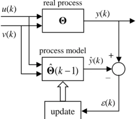
7. Wait for the next sampling time and return to step 1. Fig. 4 illustrates the idea of the Recursive Least Squares method for system identification.
Fig. 4. Illustration of the recursive estimation procedure.
III. PERSISTENT EXCITATION
For reliable parameter estimation, the output signal of the system under identification must carry representative information about the system dynamics. In other words, the input signal must excite properly the system so that its output carries rich information about the system dynamics. The ideal signal for this purpose must have an uniform power spectrum. A discrete white noise meets this requirement, however, it is an ideal model of signal. Nevertheless, it’s possible to synthetize physical signals with approximate uniform spectrum on a suitable frequency range. One of such signals is the PRBS.
A Pseudo-Random Binary Signal (PRBS) [13], is an uncorrelated binary sequence. It can be generated by a shift-register, which is binary register whose bits are moved in a FIFO (first-in first-out) manner, with a trigger frequency f0. Since a shift-register is a deterministic device, its PRBS
signal is actually predictable and cyclic (periodic). However, by choosing a suitable length (number of bits) for the shift-register, it’s possible to generate PRBS signals that persist without repetition for an arbitrary long time, even by thousands of years.
For analog applications, including a low-pass filter at the output of a PRBS generator will produce a band-limited gaussian white noise, that is, a noise with flat (uniform)
power spectrum up to the cut-off frequency of the filter. Alternatively, one may compute a weighted sum of the bits of the shift-register, using a set of resistors, with similar result. Those are some ways to generate analog signals with uniform spectrum up to several MHz. Such digitally synthetized analog noises are easy to generate using the same computer that implements the digital controller.
The simpler and more commonly used PRBS generator is the feedback shift-register, shown in Fig. 5. A shift-register with length of n bits triggered by a clock frequency f0. An
exclusive-or gate is used to generate a serial input bit to the shift-register, from its latest (nth) bit and an specific
intermediate (mth) bit. The maximum number of states for a
shift-register of length n is 2n, but the state {0
1020304…0n}
gets stuck, since the exclusive-or gate regenerates a bit 0 in the serial input of the shift-register. Therefore, the maximum number of states for this feedback shift-register is 2n–1.
Starting from a given non-zero initial state, the shift-register gets several states, eventually repeating its states history after 2n–1 clock pulses. The PRBS signal is the
binary sequence generated by the nth bit. It is cyclic with
period T0 = (2n–1)/f0. This period can be made arbitrary long
by choosing suitable values for the trigger frequency f0, the
length n of the shift-register, and the feedback bit m, so that the PSBS signal becomes an uncorrelated noise. It’s not necessary to build a physical circuit to generate a PRBS. It is easily generated by a software simulated shift-register, with the same language used to perform the identification, or with native functions of the software, like “idinput” from MATLAB®. In this work, the A/D conversion to acquire y(k)
and the D/A conversion to synthetize u(k) were implemented with a data acquisition board based on the C++ programming language. Therefore, the shift-register was also implemented in C++, within the system identification program.
Fig. 5. Feedback shift-register with length n and feedback bit m.
For system identification purposes, the system can be excited by a single PRBS signal, or by a combination of an specific input signal (e.g.: step, square wave, etc) plus a small PRBS, which will act as a persistent excitation to the process, mainly when the process is at a steady state condition, to avoid the matrix ΦTΦ in (12) becoming non-singular.
IV. SYSTEM IDENTIFICATION IN PRACTICE
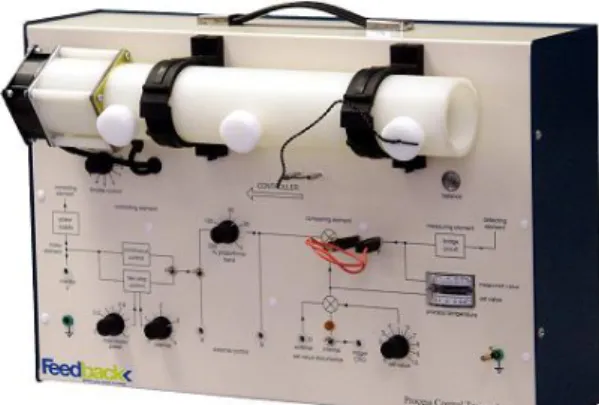
The system identification was applied to the thermal airflow system “Process Trainer PT-326” [14], by Feedback Instruments Limited, shown in Fig. 6. In this system, a rotating impeller generates an airflow through a open-end
Θ
)
1
(
ˆ
k
Θ
real process process model u(k) v(k) y(k) ) ( ˆ k y – + (k) m n–1 n 1 2 3 4 trigger PRBS 1 0 0 1…
1…
0 1 0 updateduct. The impeller rotation is manually adjusted to generate a fixed air flowrate. At the inlet of the duct, immediately after the impeller, there is a heating wire grid of Ni-Cr alloy, powered by a variable current source excited by the process input signal (or control signal), to heat the airflow generated by the impeller. The duct has three (left, central, and right) ports for insertion of a sensor (thermistor) probe into the duct, to measure the airflow temperature, which is the process variable to be controlled. A particular aspect of this thermal process is the existence of a small time-delay in the temperature response due to the displacement between the heating grid (actuator) at the inlet of the duct and the port where the thermistor probe (sensor) is inserted into the duct. Those time-delays were [15]: τ1 = 0.214 sec (left port, at 28
mm), τ2 = 0.257 sec (central port, at 140 mm), and τ3 = 0.341 sec (right port, at 274 mm). Another particular aspect is that
the process dynamics may change with variations in the external ambient air impelled into the duct. Even though those changes are small, they do exist.
A schematic of the thermal airflow system PT-326 is shown in Fig. 7. The red lines indicate the output temperature signal, which can be taken from socket “Y”. The blue lines correspond to the process input, which is delivered to the system through socket “A”. When socket “Y” is not connected to socket “X”, the system is in open loop.
The speed of the rotating impeller can be adjusted at specific fixed values by the “throttle control” dial. After fixing the impeller speed, the time delay of the airflow temperature process will depend on the location of the temperature sensor probe within the duct. In Fig. 7, the sensor probe is placed at the right port of the duct, so that the time delay of the process will be longer.
For open loop system identification, the output temperature signal is acquired by an A/D converter from socket “Y”, and the excitation signal for the process input is delivered by a D/A converter through socket “A”. Signal conditioning circuits are necessary to connect the A/D and D/A converters to the proper sockets of the system.
The Recursive Extended Least Squares (RELS) method based on the Matrix Inversion Lemma and on the UD Factorization was used to estimate the model parameters of the PT-326 system. It was observed that the step response of this system follows approximately the response of a first
order plus time-delay (FOPTD) model. For purposes of identification and control of the PT-326 system, the sampling time was chosen to be T = 0.2 sec.
For the sampling time T = 0.2 sec, the discrete model of the system was chosen as [15]:
1 1 1 1 0 2 1 ) ( ) ( ) ( z a z b b z z U z Y z GP (33)
The exact value of the time-delay exponent k depends on the sampling period T. However, since k is at least 1 (k 1), the discrete transfer function (33) can be written in a more generic form: 1 1 2 2 1 1 0 1 1 ) ( ) ( ) ( z a z b z b b z z U z Y z GP (34)
The system identification was implemented in a PC computer using the C++ programming language. A data acquisition board [1] installed in the computer provided the necessary A/D and D/A interfaces with the process to acquire the process output signal y(k) and to produce the process input signal u(k).
The identification using the RELS method was performed over 60 seconds, which corresponds to 300 sampling intervals (60/T = 60/0.2 = 300). The input signal to the system was a pure PRBS generated by software and synthetized by a D/A converter [1][2], with amplitude 0–4 volts and trigger
Fig. 7. Schematic of the thermal airflow system Process Trainer PT-326.
DOI: ISSN: period equal to the sampling period T. The first 20 seconds of
this input signal are shown in Fig. 8, and the corresponding process output is shown in Fig. 9. Recall that the output signal is the temperature of the air stream at the point where the temperature sensor is located.
Fig. 8. PRBS signal used as process input.
Fig. 9. Output temperature signal resulting from the input PRBS signal.
Fig. 10 and 11 show the results of the identification for the RELS method with UD factorization, when the system has its temperature sensor located at the right port. The initial values of all the parameters were set to 0.1. The forgetting factor for the recursive identification was set as = 0.985. The matrix U was initialized as an unity triangular superior matrix, and
the matrix D was initialized as a diagonal matrix D = 5000I. The parameters estimate resulted as:
T T 1 2 1 0 871 . 0 130 . 0 167 . 0 012 . 0 ˆ b b b a Θ (35)Fig. 10. Estimates for parameters bj.
Fig. 11. Estimate for parameter a1.
The RELS method based on the Matrix Inversion Lemma was also implemented. The same initial values for the parameter estimates and for the forgetting factor were used. The covariance matrix P was initialized as P = 5000I, and the initial values for elements of gain vector K were set to 5000. The results for the identification are shown in Fig. 12 and 13. Notice that estimates values obtained using the Matrix Inversion Lemma are statistically consistent with the values obtained with UD factorization. Compare Fig. 12 and 13 to Fig. 10 and 11. Clearly, the approach based on the Matrix Inversion Lemma is more sensitive to numerical calculations, although it was not ill-conditioned.
Fig. 12. Estimates for parameters bj (matrix inversion lemma)
Fig. 13. Estimate for parameter a1 (matrix inversion lemma)
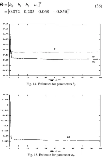
Since the identification method based on the Matrix Inversion Lemma gives imprecise results, the RELS method based on UD Factorization, due to its greater numerical robustness, was used in model identification for the two remaining positions of the temperature sensor. For the central position, the parameter estimates are shown in Fig. 14 and 15, with the following result:
T T 1 2 1 0 856 . 0 068 . 0 205 . 0 072 . 0 ˆ b b b a Θ (36)Fig. 14. Estimates for parameters bj.
Fig. 15. Estimate for parameter a1.
Finally, for the temperature sensor located at the left position, the parameter estimates are show in Fig. 16 and 17, with the following result:
T T 1 2 1 0 845 . 0 020 . 0 128 . 0 123 . 0 ˆ b b b a Θ (37)By comparing (35), (36), and (37), the absolute value of the time-constant parameter a1 decreases as the temperature
sensor is positioned more and more to the left, that is, closer and closer to the heating wire grid after the air impeller. This is consistent with the fact that the system response must become faster as the sensor gets closer to the actuator.
Fig. 16. Estimates for parameters bj.
Fig. 17. Estimate for parameter a1.
V. RECURSIVE LEAST SQUARES BASED ON THE MATRIX INVERSION LEMMA
The equations for the recursive form of the Least Squares method based on the Matrix Inversion Lemma are derived here. The covariance matrix P is defined as:
T
1 Φ Φ
P (38)
From (18), the covariance matrix at the discrete time k = N is:
T
1 1 T 1 1 1 T T 1 1 T N N N N N N N N N N N
Φ Φ Φ Φ Φ Φ P
1 T
1 1 N N N N P
P (39)Equation (39) can be expanded using the Matrix Inversion Lemma [6]:
1 1 1
1 1
1 1 DA C B DA B A A BCD A (40) By choosing: 1 1 PN A , T N
B , C1, and D
N, equation (39) can be written as:
1 1 T 1 T 1 1 1 N N N N N N N N N P P P P P T 1 1 T 1 1 1 N N N N N N N N N
P P P P P (41) Defining: T 1 1 N N N N h
P
(42) N N N N h T 1
P K (43)Notice that the Matrix Inversion Lemma allows the calculation of the covariance matrix in (41) without the need to perform matrix inversions, which is often an ill-conditioned computation.
DOI: ISSN: From (12), (18), (41), and (40), the parameters estimate
N
Θ
ˆ
at the discrete time k = N is:N N N N P Φ Y Θˆ T
N N N N N y 1 T T 1 P Φ Y
N N N N
N y T 1 T 1 P Φ Y
N N N N
N N N N N N y h T 1 T 1 1 T 1 1 Φ Y P P P N N N N N N N N N N N N N N N N N N N N h y y h T 1 T 1 T 1 1 T 1 1 T 1 1 T 1 1 P P P Y Φ P P Y Φ P N N N N N N N N N N N N N N y h h T 1 T 1 1 1 T 1 1 ˆ ˆ P P P Θ P Θ N N N N N N N N y h y T T 1 1 ˆ ˆ Θ P
P
N N N N N N N N N y h y h T 1 T 1 1 ˆ ˆ Θ P
P
N N
N N y yˆ ˆ Θ 1K N N N N Θ K
Θˆ ˆ 1 (44)where K is the vector of estimation gains, and is the
prediction error.
Equation (44) is the recursive form of the Least Squares estimation of Θ based on the Matrix Inversion Lemma.
VI. RECURSIVE LEAST SQUARES BASED ON UDFACTORIZATION
When the Bierman’s UD Factorization method is used instead of the Matrix Inversion Lemma, the Least Squares recursions follow the steps bellow:
1) Initialize matrices U and D. Let n be the number of parameters to estimate.
2) Compute the n vectors F and G as:
N N N N N N F D G U F 1 T 1 (45)
3) Set
0
, where is the forgetting factor. 4) For j = 1 to n, repeat: 1 ) 1 ( 1 ) ( 1 j j j j j j N j j N jj j j j j f g v d d g f
(46)where djj are the diagonal elements of D.
If j<1: For i = 1 to j–1 compute: j N ij N i N i j N i N ij N ij v u v v v u u ) 1 ( ) 1 ( ) ( ) 1 ( ) 1 ( ) (
(47)where uij are the upper triangular elements of U.
5) Compute the vector of estimation gains:
T 2 1 1 n n N
v v v K (48)6) Update the parameters estimate:
N N N
N Θ K
Θˆ ˆ 1 (49)
7) Wait for the next sampling time and return to step 2. Notice that when using the UD Factorization method to implement the Least Squares recursions, the covariance matrix P is not explicitly calculated. Instead, matrices D and
U are updated from their elements dj and uij in (46) and (47),
and then the gain vector K is explicitly calculated, and used to update the parameters estimate Θˆ in (49).
VII. CONCLUSION
This article presented how system identification can be used to estimate model parameters of a physical system.
The results obtained from the identification of the thermal airflow process PT-326 indicate the suitability of the Recursive Least Squares method, which can be easily applied to the identification of industrial process, provided that the process signals required by the identification can be acquired from the industrial instrumentation system. By using off-line system identification to estimate suitable models for industrial processes, those models can be used in the design of controllers, including ordinary PID controllers, for further implementation in the Plant Control System (SCADA or DCS).
Among the two mathematical approaches investigated in this work to solve the least squares identification problem, the approach based on UD Factorization showed greater numerical robustness when compared to the approach based on the Matrix Inversion Lemma. Therefore, UD Factorization should be preferable for implementing system identification applications.
The software routine developed for identification was combined with a routine for adaptive self-tuning control of the system – the second part of the work, described in a separate article.
ACKNOWLEDGMENT
The author thankfully acknowledges Dr. J.A.L. Barreiros, and Dr. Orlando “Nick” F. Silva for the helpful discussions about theoretical and practical aspects of this work.
REFERENCES
[1] ACL-812PG Enhanced Multi-Function Data Acquisition Card, ADClone Inc., 1994.
[2] ACL-812PG Software Utility and C Language Library, ADClone Inc., 1994.
[3] F. M. Hughes, “Self-Tuning and Adaptive Control: A Review of Some Basic Techniques”, Trans. Inst. MC, 1986, vol. 8, no 2, pp. 100-110. [4] G. J. Bierman, Factorization Methods for Discrete Sequential
Estimation, 1st ed. New York, USA: Academic Press, 1977.
[5] J. A. L. Barreiros, “Aplicação de Técnicas de Controle Adaptativo Auto-Ajustável à Síntese de Estabilizadores de Sistemas de Potência”, Tese de Doutorado, Departamento de Engenharia Elétrica, Universidade Federal de Santa Catarina - UFSC, Florianópolis, SC, Brasil, 1994.
[6] K. J. Åström, and B. Wittenmark, Adaptive Control, 2nd ed. Mineola, NY, USA: Dover, 2008, ch. 2, pp. 41-89.
[7] K. J. Åström, and B. Wittenmark, Computer Controlled Systems:
Theory and Design, 1st ed. Englewood Cliffs, New Jersey, USA:
Prentice-Hall International, 1996, ch. 13, pp. 505-527.
[8] K. J. Åström, U. Borisson, L. Ljung, and B. Wittenmark, “Theory and Applications of Self-Tuning Regulators”, Automatica, 1977, vol. 13, pp. 457-476. Pergamon Press.
[9] K. Ogata, Discrete-Time Control Systems, 2nd ed. Upper Saddle River, NJ, USA: Prentice-Hall International, 1995.
[10] L. Ljung, System Identification: Theory for the User, 1st ed. Englewood Cliffs, NJ, USA: Prentice-Hall, 1987, ch. 7 and 11. [11] L. Ljung, and T. Söderström, Theory and Practice of Recursive
Identification, 1st ed. Cambridge, MA, USA: The MIT Press, 1983.
[12] P. E. Wellstead, “Introduction to Self-Tuning Systems”, Lecture Notes, Control System Centre, University of Manchester Institute of Science and Technology - UMIST, Manchester, UK, 1986.
[13] P. Horowitz, and W. Hill, The Art of Electronics, 2nd ed. Cambridge, MA, USA: Cambridge University Press, 1989, pp. 655-659. [14] Process Trainer PT-326 User Manual, Feedback Instruments Limited,
Crowborough, East Sussex, England, 1996.
[15] S. A. A. Viana, “Modelamento e Controle Contínuo, Digital e Adaptativo de um Sistema de Injeção de Ar Aquecido”, Trabalho de Conclusão de Curso, Departamento de Engenharia Elétrica, Universidade Federal do Pará - UFPA, Belém, PA, Brasil, 1997. [16] T. Söderström, L. Ljung, and I. Gustavssson, “A Theoretical Analysis
of Recursive Identification Methods”, Automatica, 1978, vol. 14, pp. 231-244. Pergamon Press.
[17] T. Söderström, and P. Stoica, System Identification, 1st ed. Hertfordshire, UK: Prentice-Hall International, 1989, ch. 9, pp. 320-380.
Received: 07 November 2016 Accepted: 28 July 2017 Published: 15 August 2017
Sidney A.A. Viana was born in Belém,
PA, Brazil, in 1974. He received a Graduate degree in Electronics Engineering, in the field of Control Systems, from Universidade Federal do Pará (UFPA), Belém, PA, Brazil, in 1997; a Master of Science degree, in the fields of Control Systems and Artificial Intelligence, from Instituto Tecnológico de Aeronáutica (ITA), São José dos Campos, SP, Brazil, in 1999; and a MBA degree in Project Management, from Fundação Getúlio Vargas (FGV), Rio de Janeiro, RJ, Brazil, in 2013.
In 2000 he joined former Companhia Vale do Rio Doce (now VALE), a global mining company, where he started working in the Carajás Iron Ore Processing Plant as Instrumentation & Automation Engineer, and later as Automation Projects Engineer. In 2007 he moved to VALE’s Onça Puma Nickel Project as Lead Automation Engineer and member of the Operational Readiness Team, being responsible for the assessment of the plantwide automation system design, and keeping up with the manufacturing of the automation systems at vendors’ factories. In 2009 he joined VALE’s Paragominas Bauxite Processing Plant as Process Automation Specialist, being responsible for plant performance assessment and improvement projects, and plantwide data reconciliation. Finally, in 2013 he moved to his current position at VALE’s Ferrous Automation Engineering Department, in Belo Horizonte, MG, Brazil, where he works as Specialist Automation Engineer and Project Coordinator.
Mr. Viana was associated to the Institute of Electrical and Electronics Engineers, USA, from 1998 to 2006, when he received the grade of IEEE Senior Member, in recognition for outstanding achievements in the fields of Industrial Instrumentation, Control & Automation. He is author of several papers and technical works on Applied Control Systems, Industrial Automation, and Data Analytics. Two of his works were awarded with the first place of the Brazilian Industry Prize of the National Industry Confederation (CNI), in 2001 and 2004. His main professional interests are Industrial Engineering, industrial applications of Classical, Adaptive and Optimal Control Systems, Applied Computing, Numerical Optimization Methods, Plant Performance Management, Project Management; and Industrial Data Analytics, and Machine Learning.
© 2017 by the author. Submitted for possible open access publication under the terms and conditions of the Creative
Commons Attribution (CC-BY) license