Factores determinantes na mortalidade de vertebrados em rodovias

(1)

MESTRADO EM BIOLOGIA DA CONSERVAÇÃO

FACTORES DETERMINANTES NA

MORTALIDADE DE VERTEBRADOS EM

RODOVIAS

F

ACTORS

D

ETERMINING

V

ERTEBRATE

R

OADKILLS

Dissertação realizada por:

Filipe Granja de Carvalho

Orientador:

Prof. António Paulo Pereira Mira

Évora, 2009

(2)

UNIVERSIDADE DE ÉVORA

MESTRADO EM BIOLOGIA DA CONSERVAÇÃO

FACTORES DETERMINANTES NA

MORTALIDADE DE VERTEBRADOS EM

RODOVIAS

F

ACTORS

D

ETERMINING

V

ERTEBRATE

R

OADKILLS

Dissertação realizada por:

Filipe Granja de Carvalho

Orientador:

Prof. António Paulo Pereira Mira

Évora, 2009

(3)

ÍNDICE

Índice de Figuras ... 2 Índice de Tabelas ... 3 Resumo ... 4 Abstract ... 5 Introdução ... 6

Uma problemática globalizada ... 6

Efeitos na Biodiversidade... 6

Impacte nos vertebrados ... 8

Atenuar o problema ... 9

Objectivos ... 10

Artigo científico ... 11

Factors influencing vertebrate roadkills in Mediterranean environment: a comparison nine years later... 11 Abstract ... 11 Introduction ... 12 Study area... 13 Methods ... 16 Results ... 20 Discussion ... 29 Ackowlegements ... 34 References ... 34 Apendix I ... 39 Considerações Finais ... 41 Agradecimentos ... 44 Referências Bibliográficas ... 45

(4)

Factores determinantes da mortalidade de vertebrados em rodovias

Filipe Carvalho

₂

Índice de Figuras

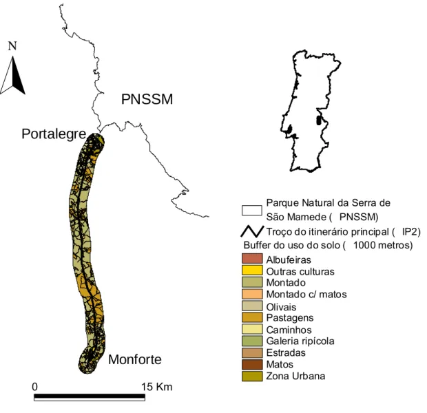
Introdução

Figura 1 – Localização do troço de estrada estudado (IP2) próximo do Parque Natural da Serra de São Mamede (PNSSM), Portugal. ... 10 Artigo científico

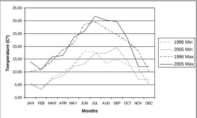
Figure 1 – Location of the studied stretch of IP2 road near the Natural Park of Serra de São Mamede (NPSSM), Portugal... 14 Figure 2 – Monthly average of minimum and maximum temperature for 1996 and 2005 in the study area (IM 2005). (The values presented correspond to the average of the 5 days before a road sampling on each month). ... 15 Figure 3 – Monthly average precipitation for 1996 and 2005 in the study area (IM, 2005). (The values presented correspond to the average of the 5 days before a road sampling on each

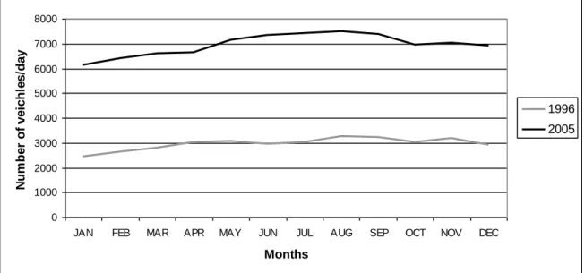
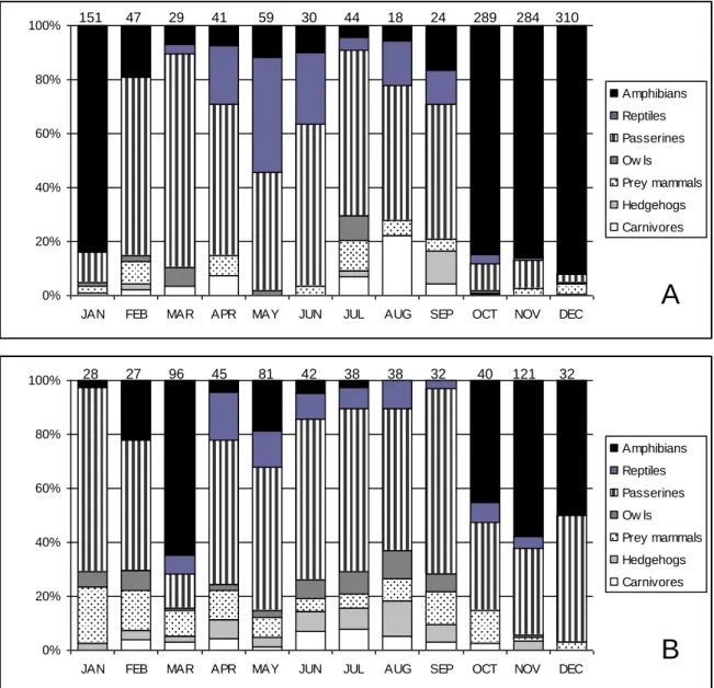
month). ... 15 Figure 4 – Monthly average on the number of cars per day in 1996 and 2005 in the studied road stretch (IEP 2000; EPE 2005). ... 16 Figure 5 – Roadkills registered along the national road section (km) in each of the two studied years. Black and grey dashed lines correspond to the average roadkills per kilometre in 1996 and 2005, respectivley. ... 23 Figure 6 – Comparisons of the monthly roadkills for ecological groups, between years: A - 1996 and B - 2005. The total number of roadkills per month is on the top of each column. ... 24 Figure 7 – Results of variation decomposition for the total vertebrate groups, showed as

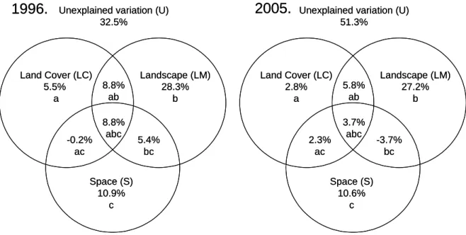
fractions of variation explained. Variation of the Ecological Vertebrate Groups (EVG) matrix is explained by three groups of explanatory variables: LC (Land cover), LM (Landscape metrics) and S (Spatial variables), and U is the unexplained variation; a, b and c are unique effects of habitat and landscape factors and spatial variables, respectively; while ab, ac, bc and abc are the components indicating their joint effects.. ... 25 Figure 8 – Ordination triplot depicting the first two axes of the environmental (total) variables partial Redundancy Analysis of the species assemblages in 1996. Environmental variables (Land cover, Landscape metrics and Spatial) (grey colour) are represented by solid lines and their acronyms (see table 3). Ecological groups’ (black colour) locations are represented by dashed arrows and their code (table 5). Samples are symbolized by black triangles. Prey_ma – prey mammals and Erinacid – hedgehogs. ... 26 Figure 9 – Ordination triplot depicting the first two axes of the environmental (total) variables partial Redundancy Analysis of the species assemblages in 2005. See details in figure 8. ... 28

(5)

Índice de Tabelas

Artigo científico

Table 1 – List of the 38 variables (two sets LC and LM) used to describe vertebrate survey roadkills locations on the road section. * Variables selected by exploratory evalutation to further analysis. ... 17 Table 2 – Number of roadkills in each of the seven ecological groups considered, by year. ... 21 Table 3 – Roadkills indexes (RKI – number of roadkills 1000 km surveyed) for each ecological groups in 1996, 2005 and total for vertebrate classes. ... 22 Table 4 – Variables selected by the manual forward procedure for each set (LC – land cover, LM – landscape metrics and S – space) for 1996 data, for inclusion in the partial Redundancy Analysis of the vertebrate groups assemblages. The conditional effects (ʎ - A), the marginal effect of each variable (ʎ - 1), the statistics of the Monte Carlo significance test for the forward procedure (F) and the associated probability (P) are reported for each variable. ... 27 Table 5 – Variables selected by the manual forward procedure for 2005 data, for inclusion in the partial Redundancy Analysis of the vertebrate groups assemblages. See details in table 4. . 28

(6)

Filipe Carvalho

₄

Factores determinantes na mortalidade de vertebrados em rodovias

Resumo

Nas últimas décadas, o incremento do número e extensão das rodovias tem contribuído para o declínio da biodiversidade em todo o mundo, principalmente devido à fragmentação dos habitats, perda de

conectividade, e mortalidade da fauna selvagem por atropelamento.

No nosso estudo, foram registados 1922 atropelamentos de vertebrados em dois anos diferentes (1326 em 1996 e 596 em 2005) num troço de 26 km entre Portalegre e Monforte de um itinerário principal (IP2). Os dados foram agrupados em sete grupos faunísticos: anfíbios, répteis, carnívoros, “mamíferos presa” (pequenos mamíferos e lagomorfos), ouriços-cacheiros, corujas e passeriformes. A identificação dos factores que mais influenciam a mortalidade de vertebrados foi efectuada através de uma análise de redundância e partição da variância, agrupando-se as variáveis em três grupos: uso dos solos, métrica da paisagem e as coordenadas espaciais dos sectores onde foram registados os atropelamentos (localização). Entre os dois anos, avaliaram-se também possíveis diferenças nos padrões de mortalidade, considerando as mudanças ao nível climático e de intensidade de tráfego.

A variância explicada em 1996 (67.5%) foi maior do que em 2005 (48.7%). Os padrões de mortalidade foram diferentes entre os anos para o total dos vertebrados, anfíbios e ouriços. A variável mais

importante, em ambos os anos, foi a distância ao Parque Natural da Serra de São Mamede (DPark). O número de atropelamentos foi gradualmente menor de norte para sul, coincidindo com um afastamento em relação aos limites do Parque Natural. A mortalidade rodoviária foi maior em áreas de montado e olivais, que estão concentradas na parte norte do troço. Em 2005, um dos anos mais secos em Portugal nas últimas décadas, outras variáveis como a distância a albufeiras (Ddam) foram significativas na explicação da mortalidade, o que sugere uma maior influência da disponibilidade hídrica nesse ano. A intensidade de tráfego foi cerca de 2.5 vezes maior em 2005, o que também pode explicar os aumentos de mortalidade de alguns dos grupos, como o ouriço-cacheiro, que foi quatro vezes superior em 2005. Por outro lado, o número de atropelamentos de anfíbios foi seis vezes menor.

Este estudo foi o primeiro que usou a partição da variância, para avaliar o contributo dos diversos grupos de variáveis nos padrões de atropelamento de vertebrados. Esta informação permitirá, no futuro aumentar a eficácia da implementação de medidas mitigadoras.

Palavras-chave: Mortalidade por atropelamento, análise de redundância, partição da variância, paisagem

(7)

Factors determining vertebrate roadkills

Abstract

In the last decades, the sudden growth of road construction has threatened biodiversity all over the world, through habitat fragmentation, reduction in connectivity and wildlife roadkills.

In our study we detected 1922 vertebrate roadkills during two different years (1326 in 1996 and 596 in 2005) in a 26 km main road stretch (IP2) between Portalegre and Monforte. We grouped the data into seven ecological groups: amphibians, reptiles, carnivores, “prey mammals” (small mammals and lagomorphs), hedgehogs, owls and passerines. The factors determining vertebrate roadkills were evaluated through redundancy analysis and variance partitioning techniques. For the analysis, variables were grouped into three sets: land cover, landscape metrics and spatial coordinates (location). We also evaluated possible differences in roadkill patterns among years, considering climatic conditions and traffic intensity changes.

The variance explained in 1996 (67.5%) was greater than in 2005 (48.7%). The roadkills patterns were different between years for total vertebrates, amphibians and hedgehogs. The most important variable, on both years, was the distance to the Natural Park of Serra de São Mamede (DPark). The roadkills decrease as we move from north to south, departing from the Natural Park. Roadkills were higher on forested areas as “montado” and olive groves, concentrated in the north part of the road stretch. In 2005, one of the driest years in Portugal in the last decades, other variables such as distance to water reservoirs (Ddam) were significant in determining roadkills, suggesting a greater water dependence on this year. Traffic intensity was 2.5 times higher in 2005, which could explain the increase of roadkills for some vertebrate groups, as hedgehogs, for which number roadkilled were four times higher in 2005. On the other hand, amphibian’s roadkills were six times lower.

To our knowledge, this study was the first one that used variance partitioning to evaluate the contribution of single variable sets on vertebrate roadkills patterns. That information, in the future, may be helpful to enhance the effectiveness of mitigation measures.

(8)

Filipe Carvalho

₆

Introdução

Uma problemática globalizada

A fragmentação de habitats e a mortalidade por atropelamento, devida à construção de infra-estruturas lineares de transporte é um dos maiores problemas ambientais à escala do planeta (Forman et al. 2003). O incessante crescimento económico e a necessidade de troca de bens entre as sociedades têm despoletado o aumento da rede rodoviária e o tráfego que nela circula a nível mundial. Em 2002, estimava-se que na Terra existiam cerca de 800.000.000 de veículos em circulação (Dargay et al. 2006). Estudos no EUA apontam para que os efeitos nefastos das estradas se estendam desde alguns metros até mais de um quilómetro em ambos os lados e que serão necessárias décadas para os avaliar (Forman & Deblinger 2000). As estradas constituem uma das maiores ameaças à biodiversidade, pondo em risco a conservação dos seres vivos em áreas por elas atravessadas e territórios adjacentes (Forman & Alexander, 1998; Trombulak & Frissel 2000; Sherwood et al. 2002; Coffin 2007). Estima-se que cerca de 5-7% de habitat das superfícies da Holanda, Bélgica e Alemanha se tenham perdido directamente devido à

construção de estradas (Jaarsma et al. 2006). Na Suécia esse valor atinge os 1.5 % (Seiler 2003) e nos EUA o valor está cifrado em 0.45 % da superfície. Se contarmos com o “road effect zone” o valor chegará aos 20% da superfície dos EUA (Forman et al. 2003).

Consequentemente a conectividade tem vindo a desaparecer das paisagens, com especial destaque para os países desenvolvidos. A manutenção da conectividade, isto é, dos corredores ecológicos entre as diferentes parcelas numa paisagem, constituirá cada vez mais um importante desafio (Crooks & Sanjayan 2006).

Efeitos na Biodiversidade

As estradas podem afectar todas as formas de vida na Terra, desde pequenos animais como as lesmas até aos mamíferos de grande porte como o alce (Alces alces) e o urso pardo (Ursus arctos) (Mumme et al. 2000; Trombular & Frissell 2000, Iuell et al. 2003; Smith-Patten & Patten 2008).

Vários são os autores que têm estudado a natureza dos efeitos das estradas na biodiversidade, enumerando diversos tipos e origens. Destes destacam-se os trabalhos de revisão elaborados por Spellerberg (1998), Forman & Alexander (1998), Trombulak & Frissel (2000), Seiler (2003) e, mais recentemente, o trabalho de Coffin (2007). Apesar de nem todos os efeitos serem

consensuais, neste trabalho destacam-se sete principais efeitos nefastos das estradas nos ecossistemas:

1. Mortalidade derivada da colisão com veículos; 2. Mortalidade derivada da construção das estradas;

(9)

4. Alteração do ambiente físico; 5. Alteração do ambiente químico; 6. Dispersão de espécies exóticas;

7. Aumento da utilização humana das áreas em que se inserem.

Dos efeitos enunciados, o efeito barreira e a colisão directa com veículos, serão os que terão maior impacte na fauna selvagem. Porém, a colisão com veículos é o mais visível para a população humana. Este afecta o efectivo populacional, quer de vertebrados quer de invertebrados. Várias medidas têm sido implementadas para reduzir os atropelamentos, no entanto, a sua eficácia está ainda longe de ser a melhor (para mais detalhes ver secção “Impacte nos vertebrados”).

A construção das estradas provoca a morte directa de organismos sésseis e de pequena

vagilidade. Prejudica também os organismos que habitam as zonas envolventes à estrada e altera o seu ambiente físico (Spellerberg 1998; Trombulak & Frissel 2000).

O efeito de barreira diminui a capacidade de movimentação dos seres vivos na paisagem entre as parcelas, podendo levar à perda da persistência e viabilidade das populações e

consequentemente à perda da biodiversidade (Forman & Alexander 1998). A presença de rodovias promove alterações de comportamento nos animais na medida em que destrói parte dos seus domínios vitais, altera as rotas de migração, diminuiu o sucesso reprodutor, compromete o estado fisiológico saudável dos animais e põe em causa a sua capacidade de fuga. Essas

alterações de comportamento contribuem para o efeito de barreira, na medida em que os animais mostram alguma relutância em atravessar as estradas (Oxley et al. 1974; Mader 1984; Mcgregor et al. 2008). Esta situação é ainda mais evidente em estradas com um fluxo de tráfego muito elevado como as auto-estradas (Reijnen et al. 1995; Clevenger et al. 2003). Assim, a restrição nas movimentações dos animais, em busca de alimento ou em dispersão, conduzirá à

diminuição da conectividade entre as populações de vertebrados. Como consequência, ocorre uma perda na diversidade genética, um aumento da consanguinidade e uma diminuição da resiliência das populações perante fenómenos estocásticos podendo levar a extinções locais (Van der Zande et al. 1980).

As estradas modificam a temperatura, a densidade e a capacidade de contenção do solo, os níveis de luminosidade, poeiras e gases, as águas superficiais e os padrões de escoamento e de sedimentação (Trombulak & Frissel 2000; Iuell et al. 2003). Por outro lado, contribuem para a contaminação das áreas adjacentes por metais pesados, sais, moléculas orgânicas, ozono e nutrientes (Trombulak & Frissel 2000; Iuell et al. 2003).

A construção destas infraestruturas promove também a dispersão de espécies exóticas porque alteram os habitats e causam stress às espécies nativas. Em contrapartida, as rodovias criam

(10)

Filipe Carvalho

₈

corredores ecológicos para as espécies exóticas e nativas aumentando o risco de atropelamento (para as espécies animais) (Spellerberg 1998; Trombulak & Frissel 2000).

Por fim, as estradas aumentam a pressão antrópica ao promoverem acessos a locais anteriormente recônditos, aumentando a perturbação passiva dos animais e promovendo mudanças ao nível da paisagem (Gratson & Whitman 2000).

Impacte nos vertebrados

O maior e mais visível impacte das estradas nos vertebrados, resulta da colisão de animais selvagens com os automóveis, principalmente quando daí resultam vítimas mortais em humanos e prejuízos avultados.

Quando a mortalidade incide em populações pequenas de espécies raras, esta pode ter consequências catastróficas na sua viabilidade (Forman & Alexander 1998). Actualmente, a mortalidade rodoviária da pantera da Florida (Puma concolor cory), atinge cerca de 49 % da população que se cifra em apenas 30-50 indivíduos (Taylor et al. 2002). A mortalidade

rodoviária é também uma importante causa de morte para os ocelotes (Leopardus pardalis) nos EUA (Cain et al. 2003), o lince-Ibérico (Lynx pardinus) em Espanha (Ferreras et al. 1992), e o lobo (Canis lupus) em Itália (Lovari et al. 2007). Na Suécia, a colisão com veículos é também a principal causa de morte dos alces (Alces alces), provocando muitas mortes em humanos e elevados prejuízos materiais (Seiler 2003). No Reino Unido, os atropelamentos são a principal causa de morte de coruja-das-torres (Tyto alba) (Rasmden 2003). Os anfíbios são talvez o grupo mais sensível ao impacte das estradas devido à elevada mortalidade a que são sujeitos durante as migrações sazonais, aquando da reprodução (Fahrig et al. 1995). Hels & Buchwald (2001), estimaram que a mortalidade por atropelamento de anfíbios se situaria entre os 34 e 63% em estradas secundárias com um fluxo baixo de tráfego e que estes valores subiriam até aos 98% em estradas muito movimentadas como as auto-estradas. Assim, algumas estradas, consoante a largura e volume de tráfego, poderão ser praticamente impermeáveis aos anfíbios (Mazerolle et al. 2005). As cobras morrem atropeladas ao serem atraídas pelo asfalto quente, funcionando a estrada como uma armadilha e levando à morte a maioria dos juvenis de um determinado ano (Rudolph et al. 1999; Andrews & Gibbons 2005). Por fim, saliente-se que a mortalidade rodoviária constitui assim um problema, que vai para além das questões conservacionistas, englobando também uma forte necessidade de gestão das espécies selvagens, segurança rodoviária e saúde pública (Groot Bruinderink & Hazebroek 1996). Com efeito, a segurança rodoviária tem sido o principal motor no sentido de reunir esforços e pressionar para a elaboração e implementação de medidas mitigadoras para a fauna selvagem (Seiler 2003).

(11)

Atenuar o problema

Um dos maiores problemas, apontado anteriormente, é a mortalidade de vertebrados em

rodovias, que tem também sido uma consequência e/ou causa do aumento do efeito barreira e da consequente perda da conectividade, potenciando a fragmentação da paisagem e das populações animais (Forman et al. 2003). Os efeitos nefastos das estradas e o despoletar gritante de

rodovias à escala global tem alertado a comunidade científica para a necessidade de investir em estudos que visem a procura de soluções e que restabeleçam a conectividade na paisagem e nas populações. Desta forma, o risco de colisão no asfalto será também atenuado.

Na resolução desta problemática, o próximo passo poderá passar por identificar os principais factores determinantes na mortalidade de vertebrados e qual a sua importância relativa. Nos últimos anos têm-se realizado alguns estudos que abordaram esta questão, quer a uma escala da paisagem, quer a uma escala local em pequenos troços, procurando a identificação de pontos negros de mortalidade (Seiler 2003; Clevenger et al. 2003; Van Langvelde & Jaarsma 2004; Malo et al. 2004). Estes pontos negros correspondem a agregações de colisões (Clevenger et al. 2003; Malo et al. 2004; Ramp et al. 2006) que reflectem os habitats específicos, o uso dos solos e a topografia nas áreas adjacentes às rodovias (Forman & Alexander 1998; Caro et al. 2000; Gomes et al. 2008). Perceber também as variações sazonais na mortalidade, que poderão ocorrer entre os diversos grupos de vertebrados, poderá oferecer o conhecimento necessário para

biólogos, engenheiros e gestores reduzirem as taxas de atropelamentos (Conrad & Gipson 2006).

Os fenómenos ecológicos resultam de numerosos factores que interagem a múltiplos níveis organizacionais em diversas escalas espaciais e temporais (Cushman & McGarigal 2002). A partição da variância é um método estatístico quantitativo, pelo qual a variabilidade nas variáveis resposta pode ser decomposta em componentes independentes. Estes reflectem a importância relativa dos diferentes grupos de descritores e os seus efeitos conjuntos (Borcard et al. 1992; Heikkinen et al. 2004). Esta técnica estatística é uma das que nos permitem modelar e encontrar os factores que mais contribuem para a mortalidade rodoviária de um ou mais grupos de vertebrados, consoante a hipótese a testar.

No futuro, com o apoio destas ferramentas, deveremos apurar de uma forma mais pragmática e fiável, quais as variáveis mais responsáveis pela morte de animais nas rodovias e assim

(12)

Filipe Carvalho

₁₀

Objectivos

Com a realização desta tese de mestrado pretende-se determinar quais os principais factores que causam a mortalidade de vertebrados em rodovias. Em concreto os principais objectivos deste trabalho são: i) Descrever os padrões de mortalidade, durante os dois anos de estudo, num troço de um itinerário principal (IP2) entre Portalegre e Monforte na Região do Alto Alentejo, Portugal (Fig. 1); ii) Quantificar a importância relativa do uso dos solos, características da paisagem e localização espacial na determinação da mortalidade rodoviária e avaliar os factores individuais que a influenciam; e por fim, iii) Comparar os padrões de mortalidade nove anos depois, entre um ano normal em termos meteriológicos (1996) e um ano de seca extrema (2005), considerando variáveis climáticas e o aumento do fluxo de tráfego entre os dois anos estudados. Estes objectivos foram desenvolvidos num artigo “Factors influencing Vertebrate Roadkills in Mediterranean environment: a comparison nine years later” a ser submetido à revista “Biodiversity and Conservation”.

Figura 1 – Localização do troço de estrada estudado (IP2) próximo do Parque Natural da Serra de São

Mamede (PNSSM), Portugal.

N

0 15 Km

PNSSM

Portalegre

Monforte

#

Buffer do uso do solo ( 1000 metros) Albufeiras Outras culturas Montado Montado c/ matos Olivais Pastagens Caminhos Galeria ripícola Estradas Matos Zona Urbana

Troço do itinerário principal ( IP2) Parque Natural da Serra de São Mamede ( PNSSM)

#

(13)

Artigo científico

FACTORS INFLUENCING VERTEBRATE ROADKILLS IN A

MEDITERRANEAN ENVIRONMENT: A COMPARISON NINE YEARS

LATER.

Filipe Carvalho *ab and António Mira ab

a

Unidade de Biologia da Conservação. Departamento de Biologia. Universidade de Évora. Núcleo da Mitra.

Apartado 94, 7002-554 Évora, Portugal. b Unidade de Ecossistemas e Paisagens Mediterrânicas. Instituto de

Ciências Agrárias Mediterrânicas. Universidade de Évora, Pólo da Mitra, 7002-554 Évora, Portugal

*_{Corresponding Author: Present address: Departamento de Biologia, Universidade de Évora, Pólo da}

Mitra, 7002-554 Évora, Portugal. Tel.:+351 919224766. E-mail address: filipescpcarvalho@yahoo.com

Abstract

Roads, due to their direct relationship with habitat loss, fragmentation and degradation, and road fatalities are one of the major threats to wildlife persistence and survivorship. We surveyed roadkills, every two weeks, on a 26 km stretch of a main national road, in two different years (1996 and 2005). For analysis proposes we grouped the data in seven vertebrates groups: amphibians, reptiles, carnivores, prey mammals (small mammals and lagomorphs), hedgehogs, owls and passerines. The main factors determining vertebrate roadkills were evaluated through Redundancy Analyses (RDA) and variance partitioning techniques, using three sets of variables: land cover (LC), landscape metrics (LM) and spatial location (S) (coordinates). We compared the patterns of vertebrate roadkills between both years surveyed, taking into account

meteorological conditions and changes in traffic intensity.

Roadkills patterns along the studied road were significantly different between years for

hedgehogs, amphibians and all vertebrates when considered together. The variance explained by the explanatory variables in 1996 was (67.5 %) greater than in 2005 (48.7 %). Many variables determining roadkills were common on both years. The most significant descriptor was the distance to the Natural Park of Serra de São Mamede (NPSSM) (DPark). The roadkills decreased gradually as we move south, away from the NPSSM border. Moreover, the results show a prevalence of the roadkills in forested areas such as “montado” and traditional olive groves, which concentrated in the north part of the road stretch. In 2005, one of the driest years in the last decades in Portugal, other important variables were selected such as distance to water reservoirs (Ddam) suggesting a greater water availability influence in these conditions. Traffic flow was 2.5 times higher in 2005 when compared with 1996 values, which might explain the increase on roadkills in almost all the groups (e.g. four times more for hedgehogs) except for amphibians that decrease approximately six times.

As far as we know our study is the first one using variance partitioning techniques to quantify the relative contribution of different sets of variables to observed roadkills patterns. That

information, in the future, may be helpful to enhance the effectiveness of mitigation measures. Key words: Roadkills, vertebrates, Mediterranean landscape, redundancy analyses, variance

(14)

Factors determining vertebrates roadkills

Filipe Carvalho and António Mira

₁₂

Introduction

One of the most visible effects of roads on wildlife is road mortality, which is a major threat to biodiversity conservation (Forman 1998; Forman and Alexander 1998; Trombulak and Frissel 2000; Sherwood et al. 2002; Forman et al. 2003; Coffin 2007). Roads can affect all kinds of life forms on Earth, from small animals such as slugs to moose and brown bears (Smith-Patten and Patten 2008). Indeed, several authors point out that roads are one of the main cause of vertebrate population decline and decrease in viability across generations (Crooks and Sanjayan 2006; Ament et al. 2008). This may be especially true for small mammals where barrier effects lead to local extinctions because of their reluctance to cross roads (Rico et al. 2007; McGregor et al. 2008). In larger and rarer species such the Iberian lynx (Lynx pardinus), the roadkills are the principal cause of death in most of the cubs in Doñana populations (Ferreras et al. 1992). In Britain, carnivores such badgers may loose 66 % of all cubs pos-emergence and adults near urban zones (Clarke et al. 1998). The principal non-natural cause of death on otters in Britain is road fatalities, which contributed to the general decline of this species (Philcox et al. 1999). In Spain barn owls have decrease 70 % in ten years, being the roadkills the principal source of deaths (Fajardo 2001). Fahrig et al. (1995) indicates that roads and traffic intensity have contributed to the global amphibian decline. Several researches have revealed negative

associations between anuran relative abundance and traffic density (Fahrig et al. 1995; Carr and Fahrig 2001; Hels and Buchwald 2001); anuran pond occupancy and road density (Vos and Chardon 1998); and amphibian species richness in breeding sites and paved road density (Findlay et al. 2001; Eigenbrod et al. 2008). Vertebrates are the most studied group in Road mortality not only for their size, but also because they comprise flagship species (Forman et al. 2003).

Understanding the explanatory factors of vertebrate roadkills, and the seasonal variations that might occur among vertebrate groups, will offer managers the knowledge to reduce collision rates and road impacts on wildlife (Saeki and Macdonald 2004; Ramp et al. 2005; Seiler 2005; Conrad and Gipson 2006). This will be accomplished, by determining and describing the location of roadkill aggregations (Clevenger et al. 2003; Ramp et al. 2006), which tend to be linked to specific habitats and landscape types in road vicinity (Forman and Alexander 1998; Caro et al. 2000; Gomes et al. 2008).

Like other ecological phenomena, roadkills are driven by numerous factors acting at multiple organizational levels, across multiple spatial and temporal scales (Cushman and McGarigal 2002). Variation partitioning is a quantitative statistical method by which the variation in the response variable(s) can be decomposed into independent components reflecting the relative importance of different groups of explanatory variables and their joint effects (Borcard et al. 1992; Heikkinen et al. 2004). We used this approach to understand the influence of land cover,

(15)

landscape metrics and spatial location on vertebrate roadkills patterns in a Mediterranean context. The partitioning method is versatile, as it can be used in a variety of univariate and multivariate contexts, with linear or unimodal response methods (Cushman and McGarigal 2002).

The main goals of our study are: i) to describe vertebrate roadkill patterns, during the two year study, in a national main road section in central Portugal; ii) to quantify the relative importance of land cover, landscape characteristics and spatial location on determining roadkills and evaluate main single factors influencing it; iii) to compare roadkills patterns in a normal and dry year, taking into account climatic changes and the increase in traffic intensity between the two studied years.

Study area

This study took place in 26 km stretch of a main road (IP2) located at Portalegre district, central Portugal. The road has two paved lanes along its entire length and runs from the central-west border of Natural Park of Serra de São Mamede (NPSSM), in Portalegre, to a small village located south (Monforte), (Fig. 1). Recently, when our field work has already been concluded, the area surrounding Monforte was classified as Special Protection Zone (DR, 1ªsérie, nº40 de 26/02/2008).

This region located near the Spanish border is generally dominated by smooth areas, except for the mountain topography of the natural Park that reaches 1024 meters above the sea level. Road vicinity is composed by a characteristic Mediterranean agro-silvo-pastoral system of cork and holm oak trees stands (Quercus suber and Quercus rotundifolia), hereafter denominated as “montado”, open land used as pasturelands, meadows, extensive agriculture, and olives groves. Road topography varies slightly along the 26 km being 30.8% levelled. 48.8% buried and 20.4 % raised, when comparing with the immediate adjacent area.

(16)

₁₄

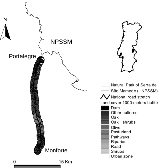
Figure 1 – Location of the studied stretch of IP2 road near the Natural Park of Serra de São Mamede

(NPSSM), Portugal.

The climate is Mediterranean with warm and dry summers and cold and rainy winters. However, 2005 was an extremely dry year, with very low precipitation levels during all year around (Fig. 2 and 3). The NPSSM is considered an Atlantic biogeographic island embedded in a Mediterranean type matrix. This biogeographic cross-road enables the coexistence of several species from both regions which contribute to a great level of biodiversity inside the Park and surrounding areas.

N

0 15 Km

NPSSM

Portalegre

Monforte

#

Land cover 1000 meters buffer Dam Other cultures Oak Oak_ shrubs Olive Pasturland Pathways Riparian Road Shrubs Urban zone

National road stretch Natural Park of Serra de São Mamede ( NPSSM)

(17)

0,00 2,00 4,00 6,00 8,00 10,00 12,00 14,00 16,00 18,00 20,00

JAN FEB MAR APR MAY JUN JUL AUG SEP OCT NOV DEC

Months P re c ip it a ti o n ( m m ) 1996 2005

Figure 2 – Monthly average of minimum and maximum temperature for 1996 and 2005 in the study area

(IM 2005). (The values presented correspond to the average of the 5 days before a road sampling on each month).

Figure 3 – Monthly average precipitation for 1996 and 2005 in the study area (IM 2005). (The values

presented correspond to the average of the 5 days before a road sampling on each month).

The studied road stretch had in 1996, less than two years after the road has been enlarged, a moderate annual daily traffic volume of 2965 vehicles day-1. In 2005 it reached high traffic intensity with an annual daily traffic volume of 6950 vehicles day-1. At both years, traffic peaks are higher in August, when compared with the rest of the year (Fig. 4).

0,00 5,00 10,00 15,00 20,00 25,00 30,00 35,00

Months Te m pe ra ture ( C º) 1996 Min 2005 Min 1996 Max 2005 Max

(18)

₁₆

Figure 4 – Monthly average on the number of cars per day in 1996 and 2005 in the studied road stretch

(IEP 2000; EPE 2005).

Methods

Roadkills survey

Roadkills were surveyed by car travelling at an average speed of 20 km/h every two weeks, from January through December, in 1996 and 2005 (26 road samplings per year). All

vertebrates found were collected and identified to the species level in loco, whenever possible, or by analysis in the laboratory of skin, scales, feathers or hairs depending on the taxonomic group. We also obtained the geographic coordinate location of all roadkills using a global positioning system (GPS) unit combined with land cover maps and detailed maps (1:2000) of road profiles. Cadavers were removed from road to avoid double counting.

Sampling units

We created a buffer of 500 meters (m) around the surveyed road and divided this polygon in 52 segments with 500 m long each, obtaining 52 rectangular sampling units (50 hectares), hereafter referred as road sectors. We choose a 500 m buffer based on the average roads effects mentioned by Forman and Deblinger (2000) and Forman et al. (2002) concerning birds, Eigenbrod et al. (2008) for amphibians and Boarman and Sazaki (2006) for reptiles. We also believe that 500m segments along the road are a good length, for the implementation of roadkills mitigation measures.

0 1000 2000 3000 4000 5000 6000 7000 8000

Months N um be r of v e ic hl e s /da y 1996 2005

(19)

Explanatory variables

Each of the 52 road segments was characterized for the 48 explanatory variables used in the present study. Variables were clustered into three groups: land cover (LC), landscape metrics (LM) and spatial coordinates (S) (table 1). Detailed Land cover maps where obtained through the interpretation of 2003 aerial photographs, complemented with fieldwork surveys. The comparison of 1995 aerial photographs with the 2003 ones revealed that only minor changes had occurred. Based on this evidence, we decided to use the same land cover map on both years. Land cover types include pasturelands, forests (comprising “montado”, old olive yards, pines and eucalyptus plantations), urban zones, aquatic areas (rivers and water reservoirs), shrublands and roads.

We used Arcview 3.2 GIS program (ESRI 1999) and the Patch analyst 2.2 (Eikie et al. 1999) extension to obtained the landscape metrics descriptors, for each segment (please see table 1 for details). Distances and all spatial descriptors were derived considering the midpoint of each 500 m road segment.

A very important landscape metric was the distance to the Natural Park of Serra de São Mamede (DPark). This variable should be interpreted as the distance to the central west limit of NPSSM which is an important natural area dominated by a mountain range NE-SW oriented. The Park is known for its high levels of humidity and rainfall and landscapes particularly well preserved. These landscapes are good examples of harmonious interactions between man and nature, maintaining high levels of biodiversity. Road topographic predictors, included in the landscape metrics set, were obtained through interpretation of detailed (1:2000) road profile maps

furnished by Estradas de Portugal, SA.

The spatial set of explanatory variables (S) consisted of 10 spatial variables including a full third-order polynomial of x and y coordinates (9 spatial variables) and an autocovariate term (Borcard et al. 1992, Heikkinen et al. 2004) in order to account for nonlinear responses:

Ẑ = b1x + b2y + b3x 2 + b4xy + b5y 2 + b6x 3 + b7x 2 y + b8xy 2 + b9y 3

Before calculating each polynomial term, the x and y coordinates were centred to zero mean to reduce collinearity between the polynomial terms (Legendre and Legendre 1998). The existence of autocorrelation in all vertebrate groups’ roadkills was evaluated using Moran’s I. When autocorrelation was detected, further analysis took this into account, using an autocovariate term (Segurado et al. 2006).

(20)

₁₈

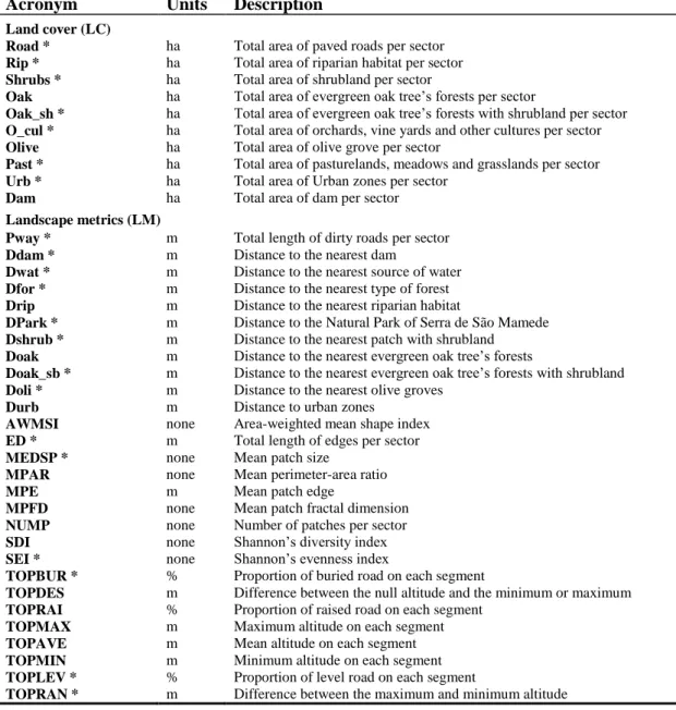
Table 1 – List of the 38 variables (two sets LC and LM) used to describe vertebrate survey roadkills locations on the road section. * Variables selected by exploratory evaluation to further analysis.

Acronym Units Description

Land cover (LC)

Road * ha Total area of paved roads per sector

Rip * ha Total area of riparian habitat per sector

Shrubs * ha Total area of shrubland per sector

Oak ha Total area of evergreen oak tree’s forests per sector

Oak_sh * ha Total area of evergreen oak tree’s forests with shrubland per sector

O_cul * ha Total area of orchards, vine yards and other cultures per sector

Olive ha Total area of olive grove per sector

Past * ha Total area of pasturelands, meadows and grasslands per sector

Urb * ha Total area of Urban zones per sector

Dam ha Total area of dam per sector

Landscape metrics (LM)

Pway * m Total length of dirty roads per sector

Ddam * m Distance to the nearest dam

Dwat * m Distance to the nearest source of water

Dfor * m Distance to the nearest type of forest

Drip m Distance to the nearest riparian habitat

DPark * m Distance to the Natural Park of Serra de São Mamede

Dshrub * m Distance to the nearest patch with shrubland

Doak m Distance to the nearest evergreen oak tree’s forests

Doak_sb * m Distance to the nearest evergreen oak tree’s forests with shrubland

Doli * m Distance to the nearest olive groves

Durb m Distance to urban zones

AWMSI none Area-weighted mean shape index

ED * m Total length of edges per sector

MEDSP * none Mean patch size

MPAR none Mean perimeter-area ratio

MPE m Mean patch edge

MPFD none Mean patch fractal dimension

NUMP none Number of patches per sector

SDI none Shannon’s diversity index

SEI * none Shannon’s evenness index

TOPBUR * % Proportion of buried road on each segment

TOPDES m Difference between the null altitude and the minimum or maximum

TOPRAI % Proportion of raised road on each segment

TOPMAX m Maximum altitude on each segment

TOPAVE m Mean altitude on each segment

TOPMIN m Minimum altitude on each segment

TOPLEV * % Proportion of level road on each segment

TOPRAN * m Difference between the maximum and minimum altitude

The autocovariate term (AUTOCOV), considers the response at one road sector as a function of the responses at neighbouring sites. It was considered for each vertebrate roadkill data group and for all vertebrates taken together (Augustin et al. 1998; Knapp et al. 2003). This term was computed using the following equations:

a) and b)

Ʃ

w

_ij

- y

_i j ≠ i

Ʃ

w

_ij

- y

_i j ≠ i

Ʃ

j ≠ i

d

_ij

-½

d

_ij

-½

Ʃ

j ≠ i

Ʃ

j ≠ i

d

_ij

-½

d

_ij

-½

(21)

Where wij is the weighted distance (meters) between the 500 meter road sector i centre and the

centre of the neighbour segment j, and yj is equal to the number of roadkills in the i segment. The weight distance was calculated by equation b), where dij is the distance (meters) between

the 500m road segment i centre and the centre of the neighbour segment j. All the distances used were calculated over the road network (Knapp et al. 2003).

Statistical analysis

For analytical purposes and to avoid a great number of zeros in the final matrix, road fatalities were aggregated into seven ecological groups (Zuur et al. 2007): amphibians, reptiles,

passerines, owls, carnivores, prey mammal and hedgehogs (table 2). The group “prey mammal” includes all small mammals and lagomorphs, due to small sample size, and their ecological affinities concerning habitat selection (both tend to concentrate on road verges) and importance in the trophic net. Hedgehogs were considered separately due to their spiny body cover, they remain on roads for a longer time than other small mammals and also because they are probably one of the most affected mammals, by road causalities all over the world (Huijser and Bergers 2000). We computed a roadkill index for each group and for all roadkills taken together, which shows the frequency of roadkills per 1000 km of road surveyed by year (Clevenger et al. 2003). For global roadkills results and for each ecological group, we tested: 1) the homogeneity (or heterogeneity) on the number of road causalities through space (road) and time (samples) on each year, using the chi-square test; 2) the significant differences between 1996 and 2005 in the road mortality pattern (peaks) along the road stretch and along the year (monthly samples), using the paired Wilcoxon test; 3) the significant differences between years, on the number of road causalities into the road stretch and samplings, using the Man-Whitney test (Sokal and Rohlf 1997). All comparisons were performed with SPSS 16.0 TM (SPSS Inc. 2008). To reduced multicollinearity we removed from further analysis the variable with the lowest biological meaning from any pair of variables having a spearman correlation coefficient higher than ± 0.70 (Tabachnik and Fidell 2001). Original variables were transformed to approach normality. We used logarithmic transformation on continuous variables (including response variables) and angular transformation for proportion land cover data (Zar 1999).

Variance partitioning

To evaluate the effects of each explanatory variable set, on the seven ecological roadkills groups, we used the variation partitioning procedure proposed by Borcard et al. (1992) extended to the three sets of variables and adapted for Redundancy Analysis (RDA) (Liu 1997; Heikkinen

(22)

₂₀

decided after running a DCA (Detrended Correspondence Analysis) on the response matrix variables for the 52 road sectors for each year data. The length of the gradient for each year (1.497 and 2.261, for 1996 and 2005, respectively), suggests that a linear method (RDA) is more appropriate to deal with our data (Jongman et al. 1995; ter Braak and Smilauer 2002; Leps and Smilauer 2003).

In first step we ran a RDA on each set of explanatory variables using a manual selection option and Monte Carlo permutation tests (499 permutations) (ter Braak and Smilauer 2002). Only the predictor variables that contribute significantly (P < 0.1), and improve the fit of RDA models were retained in the following analysis (Borcard et al. 1992, Liu 1997; Heikinnen et al. 2004). At each RDA we also test the statistical significance of all axes and the sum of all canonical eigenvalues with a Monte Carlo permutation test (499 unrestricted permutations) (ter Braak and Smilauer 2002; Leps and Smilauer 2003).

For each year data, after developing single set models and identifying explanatory variables selected, we computed three joint models, one for each of the possible combinations of every two sets; and a global model including all the variables selected on each single set model. This procedure allowed us to decompose the variance of the data into eight components: a) pure effect of land cover; b) pure effect of landscape metrics; c) pure effect of spatial component; ab) shared effect of habitat cover and landscape metrics; ac) shared effect of habitat cover and spatial component; bc) shared effect of landscape metrics and spatial components; abc) shared effect of the three groups of explanatory variables; and finally U) unexplained variation. The variance partitioning procedures were done according the methodology explained in Heikkinen et al. (2004). All multivariate analysis was performed using the program CANOCO version 4.5 (ter Braak and Smilauer 2002).

Results

Roadkills data

During the 52 road samplings (26 per year), a total of 1352 km of road were covered. We registered 2073 vertebrate roadkills belonging to 87 species (see appendix I). However, in data analysis, we only used 1922 vertebrate roadkilled belonging to 75 species, which we aggregated in previously explained seven ecological groups (table 2), after removing domestic animals and rare species that could not be include on any of the seven ecological groups considered.

In 1996 we found 63 mammals (12 species), 266 birds (29 species), 934 amphibians (10 species) and 63 reptiles (5 species) roadkilled. In 2005 we registered 95 mammals (15 species), 296 birds (32 species), 159 amphibians (8 species) and 43 reptiles (8 species).

(23)

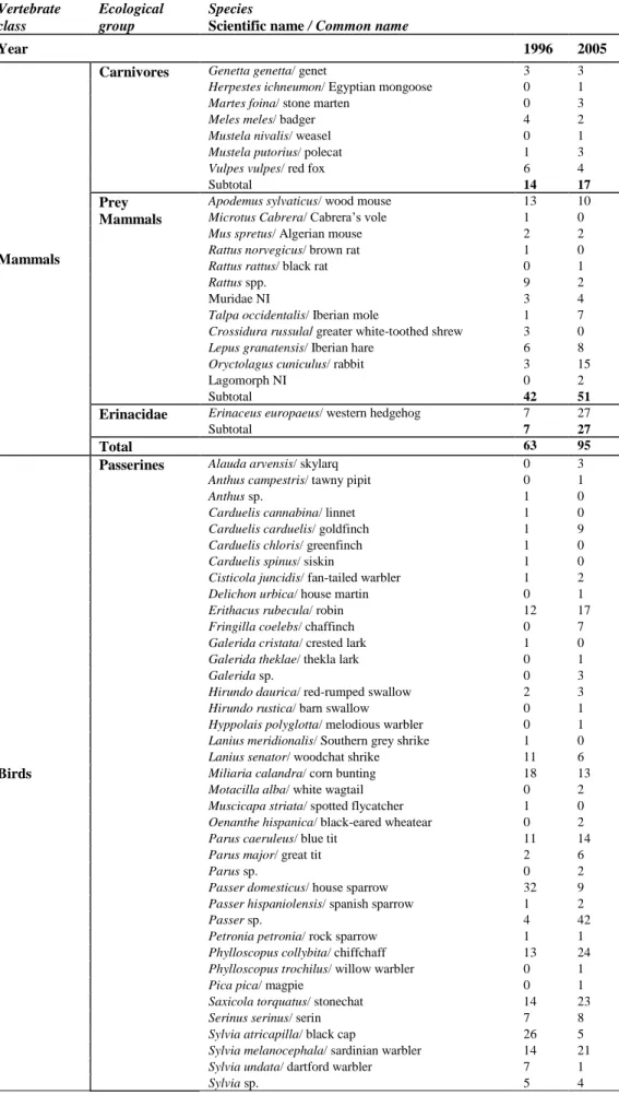
Table 2 – Number of roadkills in each of the seven ecological groups considered, by year. Vertebrate class Ecological group Species

Scientific name / Common name

Year 1996 2005

Mammals

Carnivores Genetta genetta/ genet 3 3

Herpestes ichneumon/ Egyptian mongoose 0 1

Martes foina/ stone marten 0 3

Meles meles/ badger 4 2

Mustela nivalis/ weasel 0 1

Mustela putorius/ polecat 1 3

Vulpes vulpes/ red fox 6 4

Subtotal 14 17

Prey Mammals

Apodemus sylvaticus/ wood mouse 13 10

Microtus Cabrera/ Cabrera’s vole 1 0

Mus spretus/ Algerian mouse 2 2

Rattus norvegicus/ brown rat 1 0

Rattus rattus/ black rat 0 1

Rattus spp. 9 2

Muridae NI 3 4

Talpa occidentalis/ Iberian mole 1 7

Crossidura russula/ greater white-toothed shrew 3 0

Lepus granatensis/ Iberian hare 6 8

Oryctolagus cuniculus/ rabbit 3 15

Lagomorph NI 0 2

Subtotal 42 51

Erinacidae Erinaceus europaeus/ western hedgehog 7 27

Subtotal 7 27

Total 63 95

Birds

Passerines Alauda arvensis/ skylarq 0 3

Anthus campestris/ tawny pipit 0 1

Anthus sp. 1 0

Carduelis cannabina/ linnet 1 0

Carduelis carduelis/ goldfinch 1 9

Carduelis chloris/ greenfinch 1 0

Carduelis spinus/ siskin 1 0

Cisticola juncidis/ fan-tailed warbler 1 2

Delichon urbica/ house martin 0 1

Erithacus rubecula/ robin 12 17

Fringilla coelebs/ chaffinch 0 7

Galerida cristata/ crested lark 1 0

Galerida theklae/ thekla lark 0 1

Galerida sp. 0 3

Hirundo daurica/ red-rumped swallow 2 3

Hirundo rustica/ barn swallow 0 1

Hyppolais polyglotta/ melodious warbler 0 1

Lanius meridionalis/ Southern grey shrike 1 0

Lanius senator/ woodchat shrike 11 6

Miliaria calandra/ corn bunting 18 13

Motacilla alba/ white wagtail 0 2

Muscicapa striata/ spotted flycatcher 1 0

Oenanthe hispanica/ black-eared wheatear 0 2

Parus caeruleus/ blue tit 11 14

Parus major/ great tit 2 6

Parus sp. 0 2

Passer domesticus/ house sparrow 32 9

Passer hispaniolensis/ spanish sparrow 1 2

Passer sp. 4 42

Petronia petronia/ rock sparrow 1 1

Phylloscopus collybita/ chiffchaff 13 24

Phylloscopus trochilus/ willow warbler 0 1

Pica pica/ magpie 0 1

Saxicola torquatus/ stonechat 14 23

Serinus serinus/ serin 7 8

Sylvia atricapilla/ black cap 26 5

Sylvia melanocephala/ sardinian warbler 14 21

(24)

₂₂

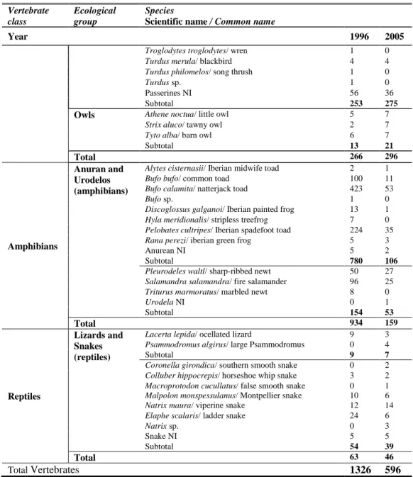
Vertebrate class

Ecological group

Species

Scientific name / Common name

Year 1996 2005

Troglodytes troglodytes/ wren 1 0

Turdus merula/ blackbird 4 4

Turdus philomelos/ song thrush 1 0

Turdus sp. 1 0

Passerines NI 56 36

Subtotal 253 275

Owls Athene noctua/ little owl 5 7

Strix aluco/ tawny owl 2 7

Tyto alba/ barn owl 6 7

Subtotal 13 21 Total 266 296 Amphibians Anuran and Urodelos (amphibians)

Alytes cisternasii/ Iberian midwife toad 2 1

Bufo bufo/ common toad 100 11

Bufo calamita/ natterjack toad 423 53

Bufo sp. 1 0

Discoglossus galganoi/ Iberian painted frog 13 1

Hyla meridionalis/ stripless treefrog 7 0

Pelobates cultripes/ Iberian spadefoot toad 224 35

Rana perezi/ iberian green frog 5 3

Anurean NI 5 2

Subtotal 780 106

Pleurodeles waltl/ sharp-ribbed newt 50 27

Salamandra salamandra/ fire salamander 96 25

Triturus marmoratus/ marbled newt 8 0

Urodela NI 0 1 Subtotal 154 53 Total 934 159 Reptiles Lizards and Snakes (reptiles)

Lacerta lepida/ ocellated lizard 9 3

Psammodromus algirus/ large Psammodromus 0 4

Subtotal 9 7

Coronella girondica/ southern smooth snake 0 2

Colluber hippocrepis/ horseshoe whip snake 3 2

Macroprotodon cucullatus/ false smooth snake 0 1

Malpolon monspessulanus/ Montpellier snake 10 6

Natrix maura/ viperine snake 12 14

Elaphe scalaris/ ladder snake 24 6

Natrix sp. 0 3

Snake NI 5 5

Subtotal 54 39

Total 63 46

Total Vertebrates 1326 596

The roadkills index (RKI) for amphibians in 1996 was the highest recorded during all the study (RKI = 690.828) (table 3). This result corresponding to 934 amphibians represents 70 % of all roadkills data in 1996 (table 3). On the other hand, in this year hedgehog had the lowest RKI (5.178), which reflects the small number of hedgehogs (only seven) found dead at this occasion (table 2). In 2005 the passerines had the highest roadkill index (RKI =203.402). In fact, 275

passerines were found dead (table 2), representing almost 46 % of the roadkills data in 2005. Table 3 – Roadkills indexes (RKI – number of roadkills per 1000 km surveyed) for each

ecological group in 1996, 2005 and total for vertebrate classes.

Year RKI by Ecological group

Total Amphibians Reptiles Passerines Owls Prey_mammals Hedgehog Carnivores

1996 990.384 690.828 46.598 187.130 9.615 31.065 5.178 10.355

2005 449.704 117.603 34.023 203.402 15.532 37.722 19.970 12.574

(25)

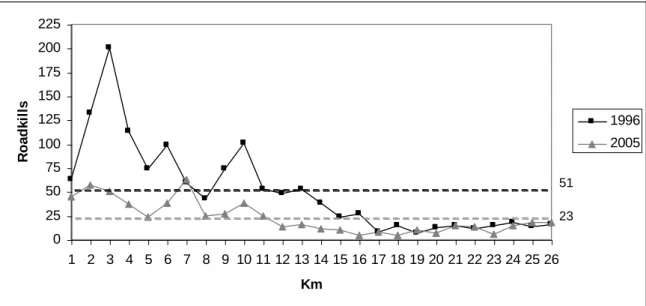
Figure 5 shows the pattern of the distribution in roadkills per road kilometre, on each year. The majority of roadkills occurred in the northern part of the road section, nearest to the Natural Park, so the heterogeneity of roadkills along the stretch was significant in 1996 and 2005 (χ²= 1077 and χ²= 3071; df. = 25; p < 0.0001, respectively).In fact, the first ten kilometres of the road captured almost 61 % and 52 % of all road casualties and include the main peaks of mortality registered on each year.

Figure 5 – Roadkills registered along the national road section (km) in each of the two studied years.

Black and grey dashed lines correspond to the average roadkills per kilometre in 1996 and 2005, respectively.

The roadkills aggregation peaks were quite similar in both years along the road (Z= -1.067; N= 26 km; p= 0.286, Wilcoxon test; Fig. 5), and through time (Z= -0.229; N= 26 samples; p= 0.819, Wilcoxon test; Fig. 6).

Comparing now the number of casualties in the road stretch between years, we verified significant differences in all vertebrates roadkills (Z=-2.426; p=0.015, Mann-Whitney test), amphibians (Z=-4.244; p<0.0001, Whitney test) and hedgehogs (Z=-2.850; p=0.004, Mann-Whitney test) (Fig. 5). Hedgehogs were also the only ecological group which showed significant differences between samplings (Z=-2.956; p=0.003, Mann-Whitney test) (Fig. 6).

Concerning temporal variation, roadkills peaks on rainy months (usually in autumn) revealing the high number of fatalities of amphibians at these occasions. This pattern was particularly marked in 1996 (Fig. 6), the year with higher rainfall (Fig. 3). On both years, summer months were usually the ones with lower mortality. In drier months, when amphibians are scarcely roadkilled, roadkills were in general higher in 2005 when compared with 1996 values (Fig. 6).

0 25 50 75 100 125 150 175 200 225 1 2 3 4 5 6 7 8 9 10 11 12 13 14 15 16 17 18 19 20 21 22 23 24 25 26 Km R o a d k il ls 1996 2005 51 23 0 25 50 75 100 125 150 175 200 225 1 2 3 4 5 6 7 8 9 10 11 12 13 14 15 16 17 18 19 20 21 22 23 24 25 26 Km R o a d k il ls 1996 2005 51 23

(26)

₂₄

Figure 6 – Comparisons of the monthly roadkills for ecological groups, between years: A - 1996 and B -

2005. The total number of roadkills per month is on the top of each column.

Variation partitioning

From the 48 initial variables, 23 were used for further analysis, after removing collinear descriptors (see table 1). Initially we used the autocovariate term to account for the

autocorrelation observed inside groups and in the overall mortality. However, this term was excluded in exploratory analysis due to the high correlation with DPark, which was easier to explain from the biological point of view.

Concerning 1996 RDA results, in the land cover set, the variables selected were: other cultures (O_cul), pasturelands (Past) and shrublands (Shrub) (table 4), altogether capturing 22.9 % of the explained variation on vertebrate roadkills (Fig. 7). From the Landscape metrics set, DPark, distance to shrublands (Dshrub), distance to forests (Dfor), length of pathways (Pway) and

0% 20% 40% 60% 80% 100%

Amphibians Reptiles Passerines Ow ls Prey mammals Hedgehogs Carnivores 0% 20% 40% 60% 80% 100%

Amphibians Reptiles Passerines Ow ls Prey mammals Hedgehogs Carnivores 151 47 29 41 59 30 44 18 24 289 284 310 28 27 96 45 81 42 38 38 32 40 121 32

A

B

0% 20% 40% 60% 80% 100%

Amphibians Reptiles Passerines Ow ls Prey mammals Hedgehogs Carnivores 151 47 29 41 59 30 44 18 24 289 284 310 28 27 96 45 81 42 38 38 32 40 121 32 0% 20% 40% 60% 80% 100%

Amphibians Reptiles Passerines Ow ls Prey mammals Hedgehogs Carnivores 151 47 29 41 59 30 44 18 24 289 284 310 28 27 96 45 81 42 38 38 32 40 121 32

A

B

(27)

distance to “montado” with shrublands (Doak_sb) (table 4) were considered significant, explaining 51.3% of the variation (Fig. 7). In the spatial set, the variables selected were: longitude coordinates (X) and longitude and latitude coordinates interaction (XY), capturing 24.9 % of the variation in the data.

In 2005 O_cul, Past, and urban zones (Urb) were the variables selected on the habitat cover set RDA (table 5), capturing 14.6% of the explained variation on road killings. In landscape metrics set, four variables were considered significant, DPark, Dfor, Doak_sb and distance to water reservoirs (Ddam) (table 5), capturing 33.0 % of the variation. In this year, three variables of spatial group were included in the RDA: X, XY and squared longitude coordinate (X2) (12.9 % of variation). When considered altogether the variables selected captured 67.5 % of the variance in 1996 and 48.7 % in 2005.

Figure 7 – Results of variation decomposition for the total vertebrate groups, showed as fractions of

variation explained. Variation of the Ecological Vertebrate Groups (EVG) matrix is explained by three groups of explanatory variables: LC (Land cover), LM (Landscape metrics) and S (Spatial variables), and U is the unexplained variation; a, b and c are unique effects of habitat and landscape factors and spatial variables, respectively; while ab, ac, bc and abc are the components indicating their joint effects.

The land cover pure effect is meaningfully higher in 1996 (5.5%) than in 2005 (2.8%). Another interesting result is the small negative value of two fractions of variance, suggesting synergism between land cover and spatial coordinates in 1996 and landscape metrics and space in 2005 (Liu 1997; Legendre and Legendre 1998). The joints effects of the three groups of variables were higher in 1996 (8.8 %) compared with the one in 2005 (3.7 %).

Land Cover (LC) 5.5% a Landscape (LM) 28.3% b Space (S) 10.9% c

Unexplained variation (U) 32.5% 8.8% ab -0.2% ac 8.8% abc 5.4% bc Land Cover (LC) 2.8% a Landscape (LM) 27.2% b Space (S) 10.6% c

Unexplained variation (U) 51.3% 5.8% ab 2.3% ac 3.7% abc -3.7% bc

1996.

2005.

Land Cover (LC) 5.5% a Landscape (LM) 28.3% b Space (S) 10.9% c

Unexplained variation (U) 32.5% 8.8% ab -0.2% ac 8.8% abc 5.4% bc Land Cover (LC) 2.8% a Landscape (LM) 27.2% b Space (S) 10.6% c

Unexplained variation (U) 51.3% 5.8% ab 2.3% ac 3.7% abc -3.7% bc

1996.

2005.

(28)

₂₆

-1.0 1.0 -1. 0 1. 0 Amphibia Reptilia Carnivor Prey_ma Erinacid Passerin Owls Past O_Cul Scrub Dscrub Pway Doak_Sb Dfor Dpark X X*Y 1 2 3 4 5 6 7 8 9 10 11 12 13 14 15 16 17 18 19 20 21 22 23 24 25 26 27 28 29 30 31 32 33 34 35 36 37 38 39 40 41 42 43 44 45 46 47 48 49 50 51 52 Axis 1 Ax is 2 -1.0 1.0 -1. 0 1. 0 Amphibia Reptilia Carnivor Prey_ma Erinacid Passerin Owls Past O_Cul Scrub Dscrub Pway Doak_Sb Dfor Dpark X X*Y 1 2 3 4 5 6 7 8 9 10 11 12 13 14 15 16 17 18 19 20 21 22 23 24 25 26 27 28 29 30 31 32 33 34 35 36 37 38 39 40 41 42 43 44 45 46 47 48 49 50 51 52 Axis 1 Ax is 2 RDA for 1996

The Monte Carlo test for the RDA of the vertebrate groups showed that the first canonical partial axis (F = 61.073, P = 0.002) and all canonical axes (F = 8.517, P = 0.002) were highly significant. Considering the vertebrate groups–environment relationship in 1996, the first two partial RDA axes captured 95.7 % of all the extracted variance (88.6% and 7.1%, respectively). The triplot graph (Fig. 8) shows that, in all groups, road mortality is negatively related to DPark, being this relationship particularly defined for prey mammals (Prey_ma), passerines (Passerin) and reptiles (Reptilia). Moreover, the higher mortality of Prey_ma, Reptilia and amphibians (Amphibia) is associated with the increasing of O_cul. Proximity to forests (decreasing on Dfor) and lower Past promotes mortality on Prey_ma, Passerin, Reptilia and Amphibia. Shrubs are highly related with owl and hedgehog fatalities.

Figure 8 – Ordination triplot depicting the first two axes of the environmental (total) variables partial

Redundancy Analysis of the species assemblages in 1996. Environmental variables (Land cover, Landscape metrics and Spatial) (grey colour) are represented by solid lines and their acronyms (see table 1). Ecological groups’ (black colour) locations are represented by dashed arrows and their code (table 4). Samples are symbolized by black triangles. Prey_ma – prey mammals and Erinacid – hedgehogs.

Mortality of Carnivores (Carnivor) also seems to increase near forest patches (decreasing Dfor), and at lower Past. Wild carnivore mortality tends to increase in areas near “montado” with shrubs, with lower length of pathway and at lower longitude (X).

(29)

The table 4 shows every variable selected during RDA analysis and their conditional effects. DPark is the most important variable related to vertebrate mortality. This importance is also stressed in the triplot where it is the variable with the longest arrow.

Table 4 – Variables selected by the manual forward procedure for each set (LC – land cover, LM – landscape metrics and S – space) for 1996 data, for inclusion in the partial Redundancy Analysis of the vertebrate groups assemblages. The conditional effects (ʎ - A), the marginal effect of each variable (ʎ - 1), the statistics of the Monte Carlo significance test for the forward procedure (F) and the associated probability (P) are reported for each variable.

RDA for 2005

The Monte Carlo test for the global RDA performed with all the descriptors included in the three single set models showed that the first canonical partial RDA axis and all canonical axes were highly significant (F = 21.002, P = 0.002 and F = 3.883; P = 0.002, respectively). The first two partial axes accounted for 88.4 % of all extracted variance (69.6 % and 18.7 %,

respectively).

The triplot (Fig. 9) for the 2005 data also shows the strong negative association between DPark and mortality of Prey_ma, Passerin, Erinacid and Owls, as in 1996. On the other hand, wild carnivore causalities present a slightly positive relation with this variable. Reptilia mortality seems to be less related with DPark, that in 1996. For the Amphibia and Reptilia, the graph suggests an increase in causalities near water reservoirs and forest patches, lower pastureland land cover and lower longitudes (X). O_Cul land cover influences the mortality patterns in the same way described for 1996 data. In 2005, Owls present an increasing number of fatalities near “montado” with shrubs areas (lower Doak_sb). However, for this vertebrate group, and to a lesser extent for Erinacid, Urban areas and XY present now a strong positive association with roadkills.

In 2005, the variable more important was also DPark, with the greatest value for conditional effects (table 5).

Set Variable ʎ - A ʎ - 1 F P-value

LC O_cul 0.04 0.10 5.790 0.012 Past 0.01 0.04 4.801 0.014 Shrub 0.01 0.06 2.836 0.052 LM DPark 0.34 0.34 26.036 0.002 Dshrub 0.01 0.10 4.804 0.016 Dfor 0.01 0.15 3.339 0.038 Pway 0.03 0.03 3.486 0.028 Doak_sb 0.04 0.03 3.242 0.038 S X 0.13 0.19 12.094 0.020 XY 0.06 0.10 3.554 0.028

(30)

₂₈

-1.0 1.0 -1. 0 1. 0 Amphibia Reptilia Carnivor Prey_ma Erinacid Passerin Owls Past O_Cul Urb Doak_Sb Dfor _Ddam Dpark X X.2 X*Y 1 2 3 4 5 6 7 8 9 10 11 12 13 14 15 16 17 18 19 20 21 22 23 24 25 26 27 28 29 30 31 32 33 34 35 36 37 38 39 40 41 42 43 44 45 46 47 48 49 50 51 52 Axis 1 Ax is 2 -1.0 1.0 -1. 0 1. 0 Amphibia Reptilia Carnivor Prey_ma Erinacid Passerin Owls Past O_Cul Urb Doak_Sb Dfor _Ddam Dpark X X.2 X*Y 1 2 3 4 5 6 7 8 9 10 11 12 13 14 15 16 17 18 19 20 21 22 23 24 25 26 27 28 29 30 31 32 33 34 35 36 37 38 39 40 41 42 43 44 45 46 47 48 49 50 51 52 Axis 1 Ax is 2

Figure 9 – Ordination triplot depicting the first two axes of the environmental (total) variables partial

Redundancy Analysis of the species assemblages in 2005. See details in figure 8.

Table 5 – Variables selected by the manual forward procedure for 2005 data, for inclusion in the partial Redundancy Analysis of the vertebrate groups assemblages. See details in table 4.

When comparing the results of both years we notice that in the global models, ten variables were selected in each case suggesting a good balance on the statistical analysis. Overall, from all the variables selected, six present strong differences in their relative importance on the results between the two years. Shrub, Dshrub and Pway were selected in 1996, but were non significant in 2005. On the other hand, Urb, Ddam, and X2 only became significant in the later year. The other seven descriptors remain common to each year model.

Set Variable ʎ - A ʎ - 1 F P-value

LC Urb 0.05 0.02 2.897 0.044 Past 0.04 0.01 2.610 0.032 O_cul 0.04 0.01 2.410 0.050 LM DPark 0.22 0.22 14.292 0.002 Dfor 0.09 0.01 2.624 0.024 Doak_sb 0.03 0.03 2.574 0.024 Ddam 0.04 0.03 2.113 0.052 S X 0.05 0.06 2.805 0.036 XY 0.03 0.10 2.060 0.098 X2 0.01 0.01 2.055 0.082