UNIVERSIDADE DE TRÁS-OS-MONTES E ALTO DOURO
SCHOOL OF SCIENCES AND TECHNOLOGY
DEPARTMENT OF ENGINEERING
Predicting Oenological Attributes Using Machine Learning
Models
Master’s Thesis in Computer Engineering
Rui Manuel Machado Silva
Advisor:
Pedro José de Melo Teixeira Pinto, Ph.D.
Universidade de Trás-os-Montes e Alto Douro
Predicting Oenological Attributes Using Machine Learning
Models
Master’s Thesis in Computer Engineering
Rui Manuel Machado Silva
Advisor:
Pedro José de Melo Teixeira Pinto, Ph.D.
Composition of the Jury:
Luís Filipe Leite Barbosa, Ph.D.
José Luís Guimarães Oliveira, Ph.D.
Pedro José de Melo Teixeira Pinto, Ph.D.
Thesis presented to the Universidade de Trás-os-Montes e Alto Douro, as a requirement to obtain a Master’s Degree in Computer Engineering under the guidance of Professor Pedro José de Melo Teixeira Pinto.
i Author’s statement: I declare that this written work has been carried out in accordance with the regulations of the
Universidade de Trás-os-Montes e Alto Douro. The work is original, except where indicated by special reference in the text. Any views expressed are those of the author and do not represent in any way the views of the Universidade de Trás-os-Montes e Alto Douro. This work, in whole or in part, was not submitted for evaluation in other Portuguese or foreign higher education institutions.
i ACKNOWLEDGEMENTS
To the magnificent dean of the University of Trás-os-Montes e Alto Douro for providing the opportunity to attend the Master’s Degree in Computer Engineering.
To the European Investment Funds by FEDER/COMPETE/POCI – Operational Competitiveness and Internacionalization Programme, under Project POCI-01-0145-FEDER-006958 and National Funds by FCT – Portuguese Foundation for Science and Technology, under the project UID/AGR/04033/2013, and through Project I&D Interact – Integrative Research in Environment, Agro-Chains and Technology, under NORTE-01-0145-FEDER-000017, in their research entitled “Fostering viticulture sustainability for Douro Valley: multidisciplinary efforts from field to wine (VitalyWINE)”, co-financed by “Fundo Europeu de Desenvolvimento Regional (FEDER)” under NORTE 2020, for their support in this investigation.
To my advisor, Professor Pedro José de Melo Teixeira Pinto, for the extreme dedication, total availability and support he provided me in the preparation of this thesis.
To my family for the support and advice that allowed me to keep the focus in ending this extensive work.
iii ABSTRACT
The potential of hyperspectral images combined with machine learning algorithms to predict anthocyanin concentration, pH index and sugar content in grapes is presented as a starting point do develop flexible models with large generalization capacity to estimate oenological parameters.
In this context, in order to evaluate the generalization capacity of the machine learning procedures, a comparison with current state of the art approaches and between three different methods, Neural Networks (NNs), Decision Trees (DTs) and Support Vector Regression (SVR), when combined with hyperspectral images, was performed to predict the anthocyanin concentration, pH index and sugar content and support the adequate monitoring of wine quality. The models were trained with six whole grape berries for each sample, using different approaches of cross-validation and data pre-processing. The oenological parameters were estimated using models trained with the spectra of 2012, 2013 and 2014 samples from the Touriga Franca variety, and the generalization capacity was tested using 2013 samples of the Tinta Barroca and Touriga Nacional varieties.
The results suggest that combining hyperspectral images with appropriate data analysis tools achieve accurate predictions. The machine learning methods were able to predict the values of oenological parameters without significant differences, improving the state of the art results.
Good indicators were obtained in the generalization capacity of the models, suggesting that a robust model capable of predicting oenological parameters on different varieties and harvest years of wine grapes can be obtained without additional training. An environmentally-friendly, fast and low-cost approach is therefore achievable and should be the subject of future testing.
Keywords: Hyperspectral Imaging, Neural Networks, Decision Trees, Support Vector Regression, Pre-Processing, Generalization.
v RESUMO
O potencial das imagens hiperespectrais combinado com algoritmos de aprendizagem máquina para prever a concentração de antocianinas, o índice pH e o teor de açúcar em uvas é apresentado, como um ponto de partida para desenvolver modelos de estimação flexíveis e com grande capacidade de generalização para estimar parâmetros enológicos.
Neste contexto, para avaliar a capacidade de generalização dos procedimentos de aprendizagem máquina, uma comparação com a literatura atual e entre três diferentes métodos,
Neural Networks (NNs), Decision Trees (DTs) e Support Vector Regression (SVR), quando
combinados com imagens hiperespectrais, foi feita para prever a concentração de antocianinas, o índice pH e o teor de açúcar e suportar a monitorização adequada da qualidade do vinho.
Os modelos foram treinados com seis bagos de uva para cada amostra, utilizando diferentes abordagens de validação cruzada e de pré-processamento dos dados. Os parâmetros enológicos foram estimados utilizando modelos treinados com espectros de amostras de 2012, 2013 e 2014, da variedade de Touriga Franca, e a capacidade de generalização foi testada com recurso a amostras de 2013 das variedades de Tinta Barroca e Touriga Nacional.
Os resultados obtidos sugerem que combinar imagens hiperespectrais com ferramentas de análise de dados apropriadas permite atingir predições precisas, sendo os métodos de aprendizagem máquina capazes de prever os valores dos parâmetros enológicos sem diferenças significativas, melhorando os resultados da literatura atual.
Foram obtidos bons indicadores sobre a capacidade de generalização dos modelos, sugerindo que um modelo robusto capaz de prever parâmetros enológicos sobre diferentes variedades e anos de colheita das uvas pode ser obtido sem treino adicional. Uma abordagem amiga do ambiente, rápida e de baixos custos é assim passível de atingir e deverá ser objeto de testes futuros.
Palavras-Chave: Imagens Hiperespectrais, Neural Networks, Decision Trees, Support Vector Regression, Pré-Processamento, Generalização.
vii GENERAL INDEX
ACKNOWLEDGEMENTS ... i
ABSTRACT ... iii
RESUMO ... v
GENERAL INDEX ... vii
TABLES INDEX ... ix
FIGURES INDEX ... xi
GRAPHS INDEX ... xiii
EQUATIONS INDEX ... xv
APPENDICES INDEX ... xix
ABBREVIATIONS AND ACRONYMS INDEX ... xxi
CHAPTER I – INTRODUCTION ... 1
1.1. Research Problem ... 1
1.2. Motivation ... 2
1.3. Objectives ... 3
CHAPTER II – STATE OF THE ART REVIEW ... 5
2.1. Prediction Methodologies in Wine Grape Berries ... 5
2.2. Other Relevant Methodologies ... 8
CHAPTER III – METHODOLOGY ... 11
3.1. Samples ... 11
3.2. Experimental Setup for Hyperspectral Images ... 14
3.3. Data Pre-Processing ... 17
3.4. Dimensionality Reduction ... 21
3.5. Model Validation ... 24
3.6. Machine Learning Algorithms ... 29
3.6.1. Neural Networks ... 30
3.6.2. Decision Trees ... 40
3.6.3. Support Vector Regression ... 45
viii
CHAPTER IV – CRITICAL ANALYSIS AND DISCUSSION ... 59
4.1. Experimental Outline ... 59
4.2. Neural Networks ... 61
4.2.1. Test Sets ... 61
4.2.2. Model Generalization ... 66
4.2.2.1. Different Vintages ... 66
4.2.2.2. Different Vintages and Varieties ... 71
4.3. Decision Trees ... 77
4.3.1. Test Sets ... 77
4.3.2. Model Generalization ... 82
4.3.2.1. Different Vintages ... 82
4.3.2.2. Different Vintages and Varieties ... 87
4.4. Support Vector Regression ... 92
4.4.1. Test Sets ... 92
4.4.2. Model Generalization ... 97
4.4.2.1. Different Vintages ... 97
4.4.2.2. Different Vintages and Varieties ... 101
4.5. Results’ Overview ... 107
CHAPTER V – CONCLUSIONS AND FUTURE WORK ... 109
BIBLIOGRAPHIC REFERENCES ... 111
ix TABLES INDEX
Table 1 – Literature results for the prediction of oenological parameters on whole grape berries, with hyperspectral imaging performed in reflectance mode ... 8 Table 2 – Descriptive statistics for the anthocyanin concentration of the laboratory results ... 12 Table 3 – Descriptive statistics for the pH index of the laboratory results ... 13 Table 4 – Descriptive statistics for the sugar content of the laboratory results ... 13 Table 5 – Results obtained for the prediction of sugar content on TF 2012 samples with different pre-processing methods ... 20 Table 6 – Results obtained for the prediction of sugar content on TF 2012 samples with and without the application of a PCA ... 23 Table 7 – Results obtained for the prediction of sugar content on TF 2012 samples with different model validation methods ... 28 Table 8 - Results obtained for the prediction of sugar content, pH index and anthocyanin concentration on TF 2012 with different NNs initialization approaches ... 39 Table 9 – Results obtained for the prediction of anthocyanin concentration, pH index and sugar content on TF 2012 with different SVR loss functions ... 50 Table 10 – Results obtained for the prediction of anthocyanin concentration, pH index and sugar content on TF 2012 samples with different kernel functions on the SVR model ... 51 Table 11 – Results obtained for the prediction of anthocyanin concentration, pH index and sugar content on TF 2012 samples with different optimization methods for the parameters on the SVR model ... 52 Table 12 – Outline of the different experiments performed in the sections below ... 60 Table 13 – Results for the determination of anthocyanin concentration on the test sets using NNs ... 62 Table 14 – Results for the determination of pH index on the test sets using NNs ... 63 Table 15 – Results for the determination of sugar content on the test sets using NNs ... 64 Table 16 – Results for the prediction of anthocyanin concentration on different vintages with NNs ... 66 Table 17 – Results for the prediction of pH index on different vintages with NNs ... 68 Table 18 – Results for the prediction of sugar content on different vintages with NNs ... 70 Table 19 – Results for the determination of anthocyanin concentration on the test sets using DTs ... 78
x Table 20 – Results for the determination of pH index on the test sets using DTs ... 79 Table 21 – Results for the determination of sugar content on the test sets using DTs ... 81 Table 22 – Results for the prediction of anthocyanin concentration on different vintages with DTs ... 83 Table 23 – Results for the prediction of pH index on different vintages with DTs ... 84 Table 24 – Results for the prediction of sugar content on different vintages with DTs ... 86 Table 25 – Results for the determination of anthocyanin concentration on the test sets using SVR ... 93 Table 26 – Results for the determination of pH index on the test sets using SVR ... 94 Table 27 – Results for the determination of sugar content on the test sets using SVR ... 95 Table 28 – Results for the prediction of anthocyanin concentration on different vintages with SVR ... 97 Table 29 – Results for the prediction of pH index on different vintages with SVR ... 99 Table 30 – Results for the prediction of sugar content on different vintages with SVR ... 100 Table 31 – Summary of the best results obtained by each of the models presented for the prediction of the oenological parameters in wine grape berries ... 107
xi FIGURES INDEX
Figure 1 – Experimental setup for hyperspectral image acquisition ... 15
Figure 2 – Data splitting in the random sub-sampling (Monte-Carlo) approach ... 24
Figure 3 – Data splitting in k-Fold Cross-Validation ... 25
Figure 4 – Example of a NN having a feed-forward topology ... 34
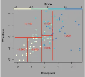
Figure 5 – Regression tree for predicting the price of 1993-model cars ... 42
Figure 6 – The partition of the data implied by the regression tree from Figure 5 ... 42
Figure 7 – The soft margin loss setting corresponds for a linear SV machine ... 47
xiii GRAPHS INDEX
Graph 1 – Reflectance measurements for the TF 2012 samples ... 17 Graph 2 – Reflectance measurements for the Touriga Franca 2012 samples; a) Original; b) After applying the Savitzky-Golay Filter ... 18 Graph 3 – Reflectance measurements for the TF 2012 samples; a) Original; b) After applying the Savitzky-Golay Filter; c) After applying the SNV transformation ... 19 Graph 4 – Scree plot of the PCA implementation for the TF 2012 reflectance measurements 22 Graph 5 – Residuals vs fit values plot for the prediction of anthocyanin concentration on the TF 2013 samples by the NNs model. ... 67 Graph 6 – Results for the estimation of anthocyanin concentration on different vintages and varieties with NNs; a) TB 2013 generalization set; b) TN 2013 generalization set ... 72 Graph 7 – Results for the estimation of pH index on different vintages and varieties with NNs; a) TB 2013 generalization set; b) TN 2013 generalization set ... 74 Graph 8 – Results for the estimation of sugar content on different vintages and varieties with NNs; a) TB 2013 generalization set; b) TN 2013 generalization set ... 76 Graph 9 – Results for the estimation of anthocyanin concentration on different vintages and varieties with DTs; a) TB 2013 generalization set; b) TN 2013 generalization set ... 87 Graph 10 – Results for the estimation of pH index on different vintages and varieties with DTs; a) TB 2013 generalization set; b) TN 2013 generalization set ... 89 Graph 11 – Results for the estimation of sugar content on different vintages and varieties with DTs; a) TB 2013 generalization set; b) TN 2013 generalization set ... 91 Graph 12 – Results for the estimation of anthocyanin concentration on different vintages and varieties with SVR; a) TB 2013 generalization set; b) TN 2013 generalization set ... 102 Graph 13 – Results for the estimation of pH index on different vintages and varieties with SVR; a) TB 2013 generalization set; b) TN 2013 generalization set ... 104 Graph 14 – Results for the estimation of sugar content on different vintages and varieties with SVR; a) TB 2013 generalization set; b) TN 2013 generalization set ... 105
xv EQUATIONS INDEX
Equation 1 – Expressing reflectance as a function of some position and wavelength ... 16 Equation 2 – Description of the convolution process in a general case ... 18 Equation 3 – Calculation of the standard normal variation at each wavelength W ... 19 Equation 4 – Mean-centering operation on a dataset 𝒚 ... 21 Equation 5 – Auto-scaling operation on a dataset 𝑿 ... 21 Equation 6 – PCA in matrix form ... 22 Equation 7 – Error of the Monte Carlo Cross-Validation method per repetition ... 25 Equation 8 – Average generalization error of the Monte-Carlo Cross-Validation ... 25 Equation 9 – Error of the k-Fold Cross-Validation method per set ... 26 Equation 10 – Error of the Bootstrap method for the learning set per experiment ... 26 Equation 11 – Error of the Bootstrap method for the validation set per experiment ... 26 Equation 12 – Average optimism computation in the Bootstrap method ... 27 Equation 13 – Learning error in the Bootstrap method ... 27 Equation 14 – Estimate of the generalization error for the Bootstrap method ... 28 Equation 15 – Linear models for regression and classification ... 30 Equation 16 – Expression of the quantities known as activations in the first layer of the network ... 31 Equation 17 – Expression of the hidden units ... 31 Equation 18 – Expression of the quantities known as activations in the second layer of the network ... 31 Equation 19 – Overall network function for sigmoidal output unit activation functions ... 32 Equation 20 – Expression of the quantities known as activations after absorbing the bias parameters into the set of weight parameters in the first layer of the network ... 32 Equation 21 – Overall network function for sigmoidal output unit activation functions after absorbing the bias parameters into the set of weight parameters ... 33 Equation 22 – Hidden or output unit function in a network... 33 Equation 23 – Condition to find the smallest value of the error function 𝑬(𝒘) ... 34 Equation 24 – Technique to optimize continuous nonlinear functions ... 35 Equation 25 – Approach to using gradient information comprising a small step in the direction of the negative gradient ... 35
xvi Equation 26 – Error function based on maximum likelihood for a set of independent observations ... 35 Equation 27 – Approach to use gradient information comprising a small step in the direction of the negative gradient for an on-line approach ... 36 Equation 28 – Weighted sum of the inputs in a general feed-forward NN ... 36 Equation 29 – Transformation of the weighted sum of the inputs by a nonlinear activation function 𝒉(∙) ... 36 Equation 30 – Evaluation of the derivatives for all the output units according to the errors 𝜹 37 Equation 31 – Backpropagation formula ... 37 Equation 32 – Evaluation of the derivatives for all the hidden units according to the errors 𝜹 ... 37 Equation 33 – Evaluation of the derivatives for each pattern in the training set ... 37 Equation 34 – Activation function chosen for the hidden units (bipolar sigmoidal function) . 38 Equation 35 – Linear regression modelling of the dependent variable 𝒀 ... 40 Equation 36 – Multiple regression modelling of the dependent variable 𝒀 ... 41 Equation 37 – Modelling of a leaf-node ... 41 Equation 38 – Sum of squared errors of a tree 𝑻 ... 43 Equation 39 – Prediction for leaf 𝒄 ... 43 Equation 39 – Sum of squared errors of a tree 𝑻 re-written to include the within-leave variance of a leaf 𝒄 ... 43 Equation 40 - Example of a linear function 𝒇. ... 45 Equation 41 - Convex optimization problem of minimizing the Euclidean norm ... 46 Equation 42 – Convex optimization problem of minimizing the Euclidean norm with slack variables to cope with otherwise infeasible constraints ... 46 Equation 43 – Description of the 𝜺-insensitive loss function ... 46 Equation 44 – Dual formulation via a Lagrange function of the objective function and the corresponding constraints ... 47 Equation 45 – Dual optimization problem ... 48 Equation 46 – Support Vector expansion ... 48 Equation 47 - Mapping the input vectors into a high-dimensional feature space. ... 49 Equation 48 – Expressing nonlinear regression functions ... 49 Equation 49 – Linear kernel function ... 49
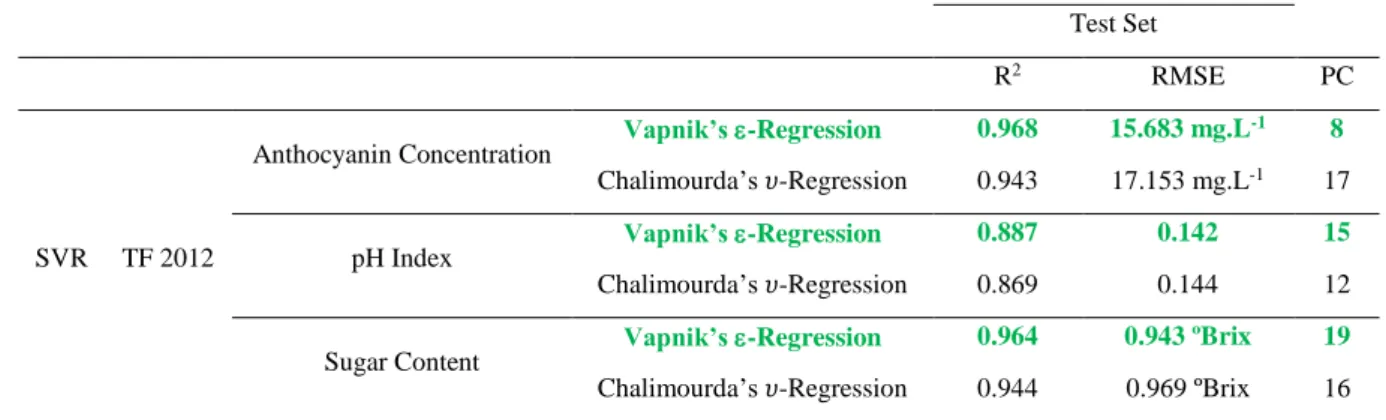
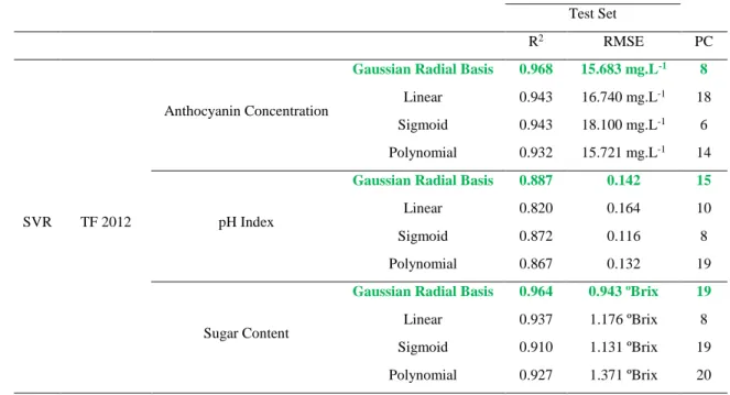
xvii Equation 50 – Sigmoid kernel function ... 49 Equation 51 – Polynomial kernel function ... 50 Equation 52 – Gaussian radial basis kernel function ... 50 Equation 53 – Calculation of R2 ... 61 Equation 54 – Calculation of RMSE ... 61
xix APPENDICES INDEX
APPENDIX A – Data distribution for the anthocyanin concentration values of the laboratory results ... 117 APPENDIX B – Boxplots for the anthocyanin concentration values of the laboratory results ... 118 APPENDIX C – Summary report of the One-Way ANOVA tests for anthocyanin values in laboratory results ... 119 APPENDIX D – Data distribution for the pH index values of the laboratory results ... 120 APPENDIX E – Boxplots for the pH index values of the laboratory results... 121 APPENDIX F – Summary report of the One-Way ANOVA tests for pH index values in laboratory results ... 122 APPENDIX G – Data distribution for the sugar content values of the laboratory results ... 123 APPENDIX H – Boxplots for the sugar content values of the laboratory results ... 124 APPENDIX I – Summary report of the One-Way ANOVA tests for sugar content values in laboratory results ... 125 APPENDIX J – Reflectance measurements for the TF 2013, TF 2014, TB 2013 and TN 2013 samples, respectively. ... 127 APPENDIX K – Descriptive statistics of the laboratory results of the samples used on the generalization sets for the NN model ... 129 APPENDIX L – Descriptive statistics of the laboratory results of the samples used on the generalization sets for the DT model ... 130 APPENDIX M – Descriptive statistics of the laboratory results of the samples used on the generalization sets for the SVR model ... 131 APPENDIX N – Residuals vs fit values plots for the prediction of pH index and sugar content, respectively, on the TF 2013 generalization set by the NN model ... 133 APPENDIX O – Residuals vs fit values plot for the prediction of pH index and sugar content, respectively, on the TF 2014 generalization set by the NN model ... 134 APPENDIX P – Residuals vs fit values plot for the prediction of anthocyanin concentration, pH index and sugar content, respectively, on the TB 2013 generalization set by the NN model ... 135
xx APPENDIX Q – Residuals vs fit values plot for the prediction of anthocyanin concentration, pH index and sugar content, respectively, on the TN 2013 generalization set by the NN model ... 137 APPENDIX R – Residuals vs fit values plot for the prediction of anthocyanin concentration, pH index and sugar content, respectively, on the TF 2013 generalization set by the DT model ... 139 APPENDIX S – Residuals vs fit values plot for the prediction of pH index and sugar content, respectively, on the TF 2014 generalization set by the DT model ... 141 APPENDIX T – Residuals vs fit values plot for the prediction of anthocyanin concentration, pH index and sugar content, respectively, on the TB 2013 generalization set by the DT model ... 143 APPENDIX U – Residuals vs fit values plot for the prediction of anthocyanin concentration, pH index and sugar content, respectively, on the TN 2013 generalization set by the DT model ... 145 APPENDIX V – Residuals vs fit values plot for the prediction of anthocyanin concentration, pH index and sugar content, respectively, on the TF 2013 generalization set by the SVR model ... 147 APPENDIX W – Residuals vs fit values plot for the prediction of pH index and sugar content, respectively, on the TF 2014 generalization set by the SVR model ... 149 APPENDIX X – Residuals vs fit values plot for the prediction of anthocyanin concentration, pH index and sugar content, respectively, on the TB 2013 generalization set by the SVR model ... 151 APPENDIX Y – Residuals vs fit values plot for the prediction of anthocyanin concentration, pH index and sugar content, respectively, on the TN 2013 generalization set by the SVR model ... 153
xxi ABBREVIATIONS AND ACRONYMS INDEX
ANOVA – One-Way Analysis of Variance. DT – Decision Tree.
MSC – Multiplicative Scatter Correction. MSE – Mean Squared Error.
NIR – Near-infrared. NN – Neural Network.
PCA – Principal Component Analysis. PLS – Partial Least Squares.
RMSE – Root Mean Squared Error. R2 – Determination Coefficient. SNV – Standard Normal Variate. SV – Support Vector.
SVR – Support Vector Regression. TB – Tinta Barroca.
TF – Touriga Franca. TN – Touriga Nacional.
1 CHAPTER I – INTRODUCTION
In an increasingly data-driven agriculture, the systematic evaluation of the quality of grapes is of major importance to the competitive market of wine production, representing an important surplus value. The Oporto wine sector (and Douro in general) has been following this evolution with the introduction of several technologies in different aspects of production, one of which is to assess non-intrusively the quality of the grapes, in particular the anthocyanin concentration, pH index and sugar content, allowing winemakers to obtain insights about their wine grapes more frequently, harvesting them at the optimal point of maturity and selecting them according to some quality features.
In this work, three machine learning models for oenological parameter estimation were implemented, namely Neural Networks (NNs), Decision Trees (DTs) and Support Vector Regression (SVR), with their efficiency and generalization capacity compared to state of the art results obtained with other machine learning algorithms and, more importantly, with purely chemometric methods like Partial Least Squares (PLS) regression. Additionally, methods to pre-process the data, smooth the spectra, reduce its dimensionality and validate the models’ results were also implemented and their effects will be discussed.
Thus, this work was split into five chapters: the first, which addresses the research problem and produces an outline of the main objectives to be completed; the second, that provides a complete state of the art review of the methods and results published in the same area of research; the third, that gives a theoretical basis on the concept of hyperspectral images and the experimental setup used, the data pre-processing step, dimensionality reduction of the data, the validation methods used and the machine learning algorithms employed for the oenological parameter estimation; the fourth, where a critical analysis and discussion of the results obtained with each model is presented; and finally, the fifth, that gives general conclusions about the work and discusses possibilities for further research.
1.1. Research Problem
Viticulture, and the entire wine industry, has undergone recent changes. As this market becomes global, competitiveness becomes one of the main challenges faced by producers. In recent years, Portugal has been one of the countries to become very competitive in the production of wines, with special focus on Port wine, whose quality is undeniable and
2 recognized throughout the world. To maintain prominence in today’s markets, it’s extremely important to ensure the high quality of the wines produced and to continue to improve the winemaking process.
The number of wine producers has increased and investment in this market has been encouraged, including the use of new technologies and methodologies to access the optimal point of maturity for grapes’ harvesting, and it’s essential to measure a number of oenological quality parameters in the grapes. In this context the anthocyanin concentration, pH index and sugar content parameters are of most importance since they have a direct influence on the quality of the wine, being related with the degree of ripening, acidity, percentage of alcohol in the wine produced, among others.
The traditional laboratory chemical analysis of grapes to assess ripening is time-consuming, costly, prone to errors and invasive (ultimately destroying grapes). With the sustained growth of computational power, new methodologies arise to deal with this problem.
“As a fast and easy-to-operate technique, infrared spectroscopy has gained wide industrial acceptance for routine wine analysis […] it is anticipated that in the near future infrared spectroscopy will progressively become a routine method for process monitoring and process control in different stages of grape and wine production” (Dambergs, Gishen, & Cozzolino, 2015, p. 261).
So, hyperspectral image-based systems, coupled with powerful data analysis tools, can be used as a viable alternative that serves, in a more consistent and objective way, the purposes of inspection, evaluation and measurement, as they are defined as fast, cost-effective and non-invasive methods.
Hence, the main problem for this work is: how to evaluate oenological parameters of grapes using environmentally-friendly, fast and cheap methods? To find ways to answer this question, there are other more specific questions that delimit this research, such as: can the machine learning models implemented reliably determine the sugar content, anthocyanin concentration and pH index with a precision similar to traditional chemical analysis?
1.2. Motivation
The present work derived from the opportunity to learn about machine learning, artificial intelligence and data processing and apply this knowledge to a real-world problem, with real applications. The interest in these emerging research fields arose early in my second year of the
3 licentiate degree when I was enrolled in a class about algorithms taught by my advisor, Professor Pedro José de Melo Teixeira Pinto, in which NNs models were one of the final topics, and it grew even more when I investigated these topics for my final licentiate project and was registered for the Machine Learning Course by Stanford University in the online education platform Coursera, taught by Professor Andrew Ng.
1.3. Objectives
The main objectives of this research were to develop three models to predict anthocyanin concentration, pH index and sugar content in grapes, with the pre-processing of the data based on available hyperspectral images, and analyse and compare the performance with the current state of the art approaches. More specifically, other requirements arose during the elaboration of the present work:
- Explain the different requirements for the proper functioning of the models.
- Ensure the validation of the predictive models based on performance estimation techniques.
- Compare the performance between machine learning algorithms and chemometric methods.
- Infer the importance of data processing (dimensionality reduction, scaling, normalization, among others) from the hyperspectral images to allow the correct analysis of the samples by the models implemented.
- Specify how to collect data from the environment setup in order to capture the hyperspectral images.
5 CHAPTER II – STATE OF THE ART REVIEW
“Hyperspectral imaging (Gowen, O’Donnell, Cullen, Downey, & Frias, 2007; Hall, Lamb, Holzapfel, & Louis, 2002) is a technique that collects information concerning how objects reflect and absorb light as a function of their wavelength” (as cited in Fernandes et al., 2011, p. 216), providing both spatial and spectral information – however, it involves complex data that requires powerful analysis tools to extract the necessary information from the underlying patterns in the spectra. In this chapter, it’ll be provided a full review of the state-of-the-art methodologies that combine hyperspectral images and data analysis tools to predict anthocyanin concentration, pH index and sugar content on grapes, and a brief review of similar methodologies that intend to perform predictions on other chemical compounds on grapes and other fruits and vegetables.
Part of this work has been submitted by the author to a scientific journal.
2.1. Prediction Methodologies in Wine Grape Berries
“In the process of analysis and evaluation of wine grapes, anthocyanin concentration, pH index and sugar content are highly researched parameters because they are correlated with the flavour, colour and are good indicators of the grapes’ ripeness” (Silva, Gomes, Faia & Melo-Pinto, 2016, para. 3). In the last years, the use of such parameters has been proposed, using different near-infrared (NIR) spectroscopy techniques: transmittance mode, “where the fruit surface viewed by the detector is diametrically opposite to the illuminated surface” (Schaare & Fraser, 2000, p. 175); interactance mode, “where the field of view of the detector is separated from the illuminated surface by a light seal in contact with the fruit surface” (idem, ibidem); and reflectance mode, “where the field of view of the light detector includes parts of the fruit surface directly illuminated by the source” (idem, ibidem).
To ease the comparison between authors, the works reviewed are separated by the spectroscopy technique used:
a) transmittance mode spectroscopy: Fernández-Novales, López, Sánchez, García-Mesa, and González-Caballero (2009) used a miniature fibre-optic NIR spectrometer system on the spectral region of 700-1060nm with a chemometric method, PLS regression, to measure sugar content and pH index; Geraudie and Ojeda (2010)measured the anthocyanin concentration on wine grape berries using
6 a combination of multiple linear regression for prediction and a Principal Component Analysis (PCA) for dimensionality reduction.
b) interactance mode spectroscopy: Herrera, Guesalaga, and Agosin (2003)developed an approach to predict sugar content on wine grape berries, using 146 samples on the 800-1050nm NIR region, alongside models with multiple linear regression and PLS regression; Larraín, Guesalaga, and Agosin (2008) measured sugar content, pH index and anthocyanin concentration, on the NIR region of up to 1100nm, using PLS regression; Geraudie et al. (2009) as mentioned previously, built models with multiple linear regression and a PCA for dimensionality reduction, in this study to measure sugar (and water) content.
c) reflectance mode spectroscopy: in the present work, it’s more relevant to analyse previous results in reflectance mode spectroscopy, since it follows the same methodology used in this study. The works in reflectance mode can be further divided into:
a. reflectance mode for a small number of berries in each sample: Arana, Jarén, and Arazuri (2005) implemented a model with PLS regression to measure the sugar content on the NIR region of 500-800nm; Wu, Huang, and He (2008) built a model combining PLS for dimensionality reduction (extracting the three best principal factors) and NNs for the prediction of sugar content; Cao, Wu, and He (2010) used a genetic algorithm to analyse the sugar content and pH index on wine grapes, processing both the whole spectra and selected wavelengths; Fernandes et al. (2015, 2011) used adaptive boosting NNs to measure anthocyanin concentration on a first approach and a classic NNs model to predict anthocyanin concentration, pH index and sugar content on the latest, on the NIR region of 380-1028nm; Gomes, Fernandes, and Melo-Pinto (2017b); Gomes, Fernandes, Faia, and Melo-Pinto (2014a, 2014b) compared the effectiveness of both, NNs and PLS regression, for the prediction of sugar content on the NIR region of 380-1028nm;
b. reflectance mode for a large number of berries in each sample: Cozzolino et
7 NIR region of 400-2500nm; Janik, Cozzolino, Dambergs, Cynkar, and Gishen (2007) compared the performance of NNs using both a PCA and PLS for dimensionality reduction on the prediction of anthocyanin concentration; Le Moigne et al. (2008) measured the anthocyanin concentration (among other parameters) on the NIR region of 250-310nm using PLS regression; Ferrer-Gallego, Hernández-Hierro, Rivas-Gonzalo, and Escribano-Bailón (2011) developed a modified PLS regression model to estimate the anthocyanin concentration on wine grapes; González-Caballero, Pérez-Marín, López, and Sánchez (2011) built a model with modified PLS regression operating on the 380-1700nm NIR region to predict sugar content and pH index; Hernández-Hierro, Nogales-Bueno, Rodríguez-Pulido, and Heredia (2013) used a modified PLS regression algorithm to measure the anthocyanin concentration on the 900-1700nm NIR region; Nogales-Bueno, Hernández-Hierro, Rodríguez-Pulido, and Heredia (2014) measured the sugar content and the pH index using a modified PLS regression model on the 900-1700nm NIR region; Chen et al. (2015)built two different models, using PLS regression and SVR, to predict the pH index and anthocyanin concentration on the 900-1700nm NIR region; Fadock, Brown, and Reynolds (2016) used PLS regression on the 350-850nm NIR region to predict sugar content, pH index and anthocyanin concentration.
It’s important to mention that the use of a larger number of berries represents a simpler problem than for a small number of berries, since the variability in berries spectra and reference oenological values evaluated attenuate along with the number of berries.
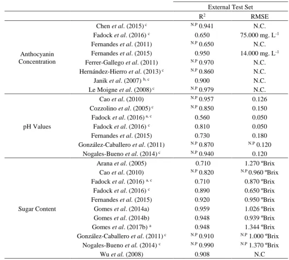
Table 1 summarizes the most relevant results obtained by each of the aforementioned authors using hyperspectral imaging in reflectance mode.
8
Table 1 – Literature results for the prediction of oenological parameters on whole grape berries, with hyperspectral imaging performed in reflectance mode
External Test Set
R2 RMSE Anthocyanin Concentration Chen et al. (2015) c N.P 0.941 N.C. Fadock et al. (2016) c 0.650 75.000 mg. L-1 Fernandes et al. (2011) N.P 0.650 N.C. Fernandes et al. (2015) 0.950 14.000 mg. L-1 Ferrer-Gallego et al. (2011) N.P 0.970 N.C. Hernández-Hierro et al. (2013) c N.P 0.860 N.C. Janik et al. (2007) b, c 0.900 N.C. Le Moigne et al. (2008) c N.P 0.979 N.C. pH Values Cao et al. (2010) N.P 0.957 0.126 Cozzolino et al. (2005) c N.P 0.850 0.150 Fadock et al. (2016) a, c 0.560 0.050 Fadock et al. (2016) c 0.810 0.050 Fernandes et al. (2015) 0.730 0.180 González-Caballero et al. (2011) N.P 0.870 N.P 0.120 Nogales-Bueno et al. (2014) c N.P 0.940 0.120 Sugar Content
Arana et al. (2005) 0.710 1.270 ºBrix
Cao et al. (2010) N.P 0.820 N.P 0.960 ºBrix
Fadock et al. (2016) a, c 0.710 0.870 ºBrix
Fadock et al. (2016) c 0.890 0.650 ºBrix
Fernandes et al. (2015) 0.920 0.950 ºBrix
Gomes et al. (2014a) 0.959 1.026 ºBrix
Gomes et al. (2014b) 0.948 0.939 ºBrix
Gomes et al. (2017b) a 0.948 1.344 ºBrix
González-Caballero et al. (2011) c N.P 0.910 N.P 1.000 ºBrix
Nogales-Bueno et al. (2014) c N.P 0.990 N.P 1.370 ºBrix
Wu et al. (2008) 0.908 N.C
a: Different vintage used in the external test set (generalization set). b: Different vintage and variety used in the external test set (generalization set). c: Large number of berries. N.P: Not provided for external test set. N.C: Not comparable.
2.2. Other Relevant Methodologies
Some other works can be found, but to measure different chemical compounds on wine grape berries and other fruits (i.e. phenolic compounds, solid sugar compounds or aroma compounds). Noguerol-Pato, González-Barreiro, Cancho-Grande, Martínez, et al. (2012); Noguerol-Pato, González-Barreiro, Cancho-Grande, Santiago, et al. (2012); Noguerol-Pato, González-Barreiro, Simal-Gándara, et al. (2012) built various approaches to study aroma compounds on different varieties of wine grape berries, using gas chromatography and mass spectrometry to determine the aromatic composition; Tarter and Keuter (2005)research focused on the differences in solid sugar compounds between the berries in different positions (top, middle and bottom) of a cluster.
9 Additionally, the use and effectiveness of support vector machines combined with hyperspectral imaging has already been tested and widely employed on classification problems; i.e., Melgani and Bruzzone (2004) addressed the problem of classification of hyperspectral remote sensing images comparing the effectiveness of support vector machines in hyperdimensional feature spaces with conventional feature-reduction-based approaches (radial basis function NNs and k-nearest neighbour classifiers); Mercier and Lennon (2003)presented modified kernels that take into consideration the spectral similarity between support vectors, applying them to images of an intensive agricultural region in France, selecting 17 bands from 450-950nm spectral data; Rumpf et al. (2010) used support vector machines for the early detection of plant diseases based on hyperspectral images obtained in reflectance mode; but approaches for regression are still slightly uncommon.
11 CHAPTER III – METHODOLOGY
In this chapter, a clear description of the samples is given alongside a theoretical basis about the experimental setup for hyperspectral images, the data pre-processing, dimensionality reduction and model validation methods used and the machine learning algorithms employed, as a form of exposing and justifying the entire process that leads to the build-up of the prediction models that provide the final results regarding the anthocyanin concentration, pH index and sugar content on wine grape berries.
A One-Way Analysis of Variance (ANOVA) was performed to study whether there are any statistically significant differences between the means of the different sets of samples. For a complete description and mathematical formulation about the ANOVA method, consult Christensen (2011). The prediction models were developed using Matlab software (The Mathworks, 2016) and the descriptive statistics, boxplots and one-way ANOVA tests used to study samples were obtained with Minitab Software (State College PA, 2010).
Part of this work has been submitted by the author to a scientific journal.
3.1. Samples
The main subjects of this study were grape bunches of the Touriga Franca (TF) variety, widely recognized as one of the most important varieties for the production of Port wine in the Douro region due to its resiliency to plant diseases, fruity flavour and intense colour, harvested from the vineyards of Quinta do Bonfim in Pinhão, Portugal, in the years of 2012, 2013 and 2014, which is property of Symington Family Estates. In order to test the generalization capacity of the models (that is, the models’ ability to predict values outside the known grape bunches used on the training process), samples from the Tinta Barroca (TB) and Touriga Nacional (TN) varieties were also collected on the year of 2013. To obtain the best possible training and testing setups, with an adequate range of values that represent grapes in different ripening stages, “it’s important to test grapes between the beginning of veraison (transition from berry growth to berry ripening) and maturity, and from areas within the same vineyard under different conditions (sun exposition, water availability, soil quality, among others)” (Silva et
al., 2016, para. 5): consequently, 240 samples were collected in the year of 2012 (24 per day),
84 in the year of 2013 (12 per day) and 120 in the year of 2014 (12 per day) from the TF variety; 84 samples (12 per day) and 60 samples (12 per day) were collected in the year of 2013 from
12 the TB and TN varieties; all of which from three different regions on the vineyard considering vine trees with small, medium and large vigour.
The hyperspectral image acquisition was performed on fresh grape berries: “each sample measured by hyperspectral imaging was composed of six grape berries randomly collected in a single bunch. The berries were removed from bunches with their pedicel still attached […] all the samples were kept frozen, at -18ºC” (Gomes et al., 2014b, p. 2).
The chemical analysis was carried out with the six grape berries being defrosted at room temperature and then
“crushed in a buffer solution of tartaric acid (pH 3.2) and ethanol (95%), by macerating, and the resulting mixture was kept overnight at 25ºC (Carbonneau & Champagnol, 1993); a centrifugation (SIGMA centrifuge 3K18, 20 min, 4ºC, spin at 7155g) was applied and a clear extract was collected and mixed with acidified ethanol (0.1% HCL)” (as cited in Gomes et al., 2014b, p. 2).
Riberéau-Gayon and Stonestreet (1965) and Office International de la Vigne et du Vin (1990) indicates that:
“The total anthocyanin concentration was determined photometrically by SO2 bleaching method (Riberéau-Gayon & Stonestreet, 1965). UV/VIS spectrophotometer (Shimadzu) and 1 cm path length, disposable cells were used for spectral measurements at 520 nm and the pigment content, expressed in mg.L-1, was calculated from a calibration curve of malvidin-glucoside. All
determinations were performed in duplicate and the juice released was analysed for the pH contents according to validated standard methods (Office International de la Vigne et du Vin, 1990, as cited in Gomes et al., 2017a, p. 42)”.
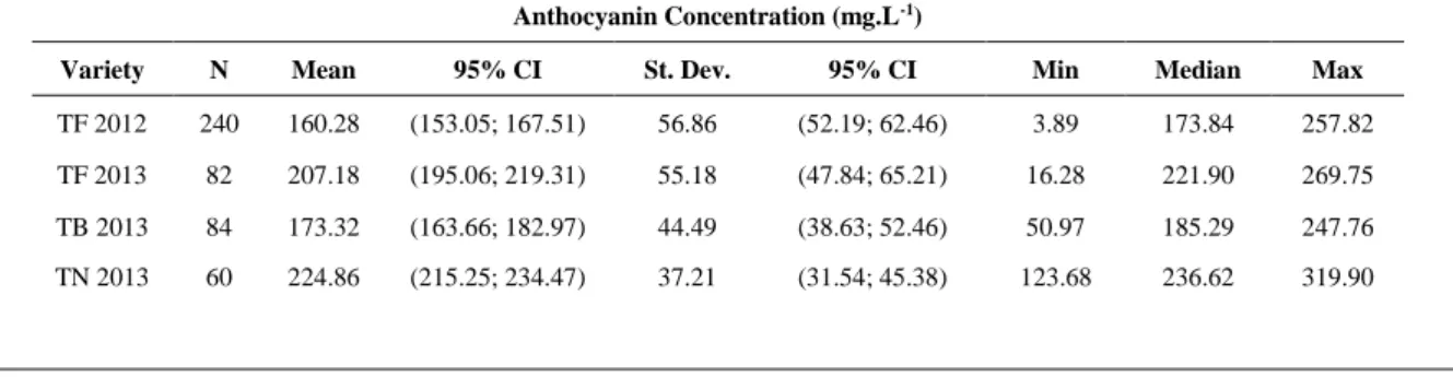
Tables 2, 3 and 4 provide descriptive statistics regarding the laboratory results of all the samples collected, on anthocyanin concentration, pH index and sugar content, respectively. Appendices A through I contain additional statistics, boxplots and one-way ANOVA tests of these values for a more detailed view of the data behaviour. For the TF variety in the 2014 vintage, there aren’t any laboratory results available regarding anthocyanin concentration.
Table 2 – Descriptive statistics for the anthocyanin concentration of the laboratory results Anthocyanin Concentration (mg.L-1)
Variety N Mean 95% CI St. Dev. 95% CI Min Median Max
TF 2012 240 160.28 (153.05; 167.51) 56.86 (52.19; 62.46) 3.89 173.84 257.82 TF 2013 82 207.18 (195.06; 219.31) 55.18 (47.84; 65.21) 16.28 221.90 269.75 TB 2013 84 173.32 (163.66; 182.97) 44.49 (38.63; 52.46) 50.97 185.29 247.76 TN 2013 60 224.86 (215.25; 234.47) 37.21 (31.54; 45.38) 123.68 236.62 319.90
13 Regarding the anthocyanin concentration values, Table 2 shows that the range of values in the different datasets are distinct, with very different means and standard deviation interval values in all populations. Appendix A clearly shows that there are outliers (observations that lie an abnormal distance from other values in a random sample from a population) in all datasets, while Appendix B allows to find differences in the centre, shape and variability among all boxplots – conducting an ANOVA test between datasets (Appendix C), it was found that there are significant differences among the means between the TF 2012 and TB 2013 samples and TF 2013 and TN 2013 samples.
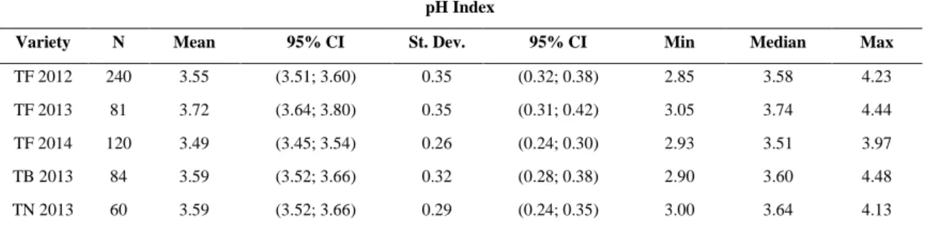
Table 3 – Descriptive statistics for the pH index of the laboratory results pH Index
Variety N Mean 95% CI St. Dev. 95% CI Min Median Max
TF 2012 240 3.55 (3.51; 3.60) 0.35 (0.32; 0.38) 2.85 3.58 4.23 TF 2013 81 3.72 (3.64; 3.80) 0.35 (0.31; 0.42) 3.05 3.74 4.44 TF 2014 120 3.49 (3.45; 3.54) 0.26 (0.24; 0.30) 2.93 3.51 3.97 TB 2013 84 3.59 (3.52; 3.66) 0.32 (0.28; 0.38) 2.90 3.60 4.48 TN 2013 60 3.59 (3.52; 3.66) 0.29 (0.24; 0.35) 3.00 3.64 4.13
As for the pH index values, Table 3 evidences a small range of values in the different datasets, with similar means and standard deviation interval values for all sets. Appendix D shows that outliers couldn’t be found in these samples, while observing Appendix E shows that the centre, shape and variability among all boxplots is very uniform – conducting an ANOVA test between datasets (Appendix F), it was still found that there are significant differences in the means between the TF 2013 samples and the TF 2012 and TF 2014 samples.
Table 4 – Descriptive statistics for the sugar content of the laboratory results Sugar Content (ºBrix)
Variety N Mean 95% CI St. Dev. 95% CI Min Median Max
TF 2012 240 16.93 (16.50; 17.35) 3.34 (3.07; 3.67) 9.06 17.06 24.72 TF 2013 82 19.45 (18.66; 20.23) 3.59 (3.11; 4.24) 8.10 20.03 25.00 TF 2014 120 13.55 (12.89; 14.21) 3.66 (3.25; 4.20) 7.87 13.00 25.66 TB 2013 84 22.49 (21.51; 23.47) 4.52 (3.92; 5.32) 11.40 23.44 30.85 TN 2013 60 23.26 (22.63; 23.89) 2.44 (2.07; 2.97) 17.20 23.84 27.20
14 Finally, studying the sugar content values, it’s possible to conclude from Table 4 that all datasets have very unique descriptive statistics, with creased differences in the range of values, means and standard deviation interval values. Appendix G shows that outliers can be found for the datasets composed of TF 2013 and TF 2014 samples, while Appendix H shows very distinct centres, shape and variability among all boxplots – the ANOVA test between datasets (Appendix I) found significant differences in the means between TF 2012, TF 2013 and TF 2014 and all the other datasets, while the TB 2013 and TN 2013 varieties have significant differences in the means when compared to all harvest years of the TF variety.
The ANOVA tests allow an important detail to come into consideration, as the models will operate predictions on datasets with statistically different means and it should influence the result analysis made in Chapter IV. The outliers found in the different datasets were kept as part of future analysis, since it’s very likely that outliers will always be found in further testing with new datasets from different varieties and vintages, and the model must be ready to reduce the importance of these values when composing a set of predictions.
3.2. Experimental Setup for Hyperspectral Images
As mentioned in Chapter II, hyperspectral imaging can be performed using different NIR spectroscopy techniques: transmittance mode, “where the fruit surface viewed by the detector is diametrically opposite to the illuminated surface” (Schaare & Fraser, 2000, p. 175); interactance mode, “where the field of view of the detector is separated from the illuminated surface by a light seal in contact with the fruit surface” (idem, ibidem); and reflectance mode, “where the field of view of the light detector includes parts of the fruit surface directly illuminated by the source” (idem, ibidem). In the present work, reflectance mode was chosen over transmittance and interactance mode since, for the same illumination scenario, the intensity of light coming from the grape is stronger, which facilitates measurements.
The experimental setup assembled for the images collected was:
“a hyperspectral camera, composed of a JAI Pulnix (JAI, Yokohama, Japan) black and white camera and a Specim Imspector V10E spectrograph (Specim, Oulu, Finland); lighting, by means of a lamp holder with 300x300x175 mms (length x width x height) that held four 20W, 12V halogen lamps and two 40W, 220V blue reflector lamps (Spotline, Philips, Eindhoven, Netherlands). Both types of lamps were powered by continuous current power supplies to avoid light flickering and the reflector lamps were powered at only 110V to reduce lighting and prevent camera saturation” (Gomes et al., 2014b, p.3).
15 The resulting hyperspectral images correspond to a single line over the sample and had 1040 wavelengths (ranging between 380 to 1028 nm, with approximately 0.6 nm of width in each channel) x 1392 pixels.
“The 1392 pixels stand for the spatial dimension over the samples with approximately 110 mm of width. The distance between the camera and the sample base was 420 mm. The camera was controlled with Coyote software from JAI inside a dark room. All the hyperspectral measurements were done at room temperature” (Gomes et al., 2014b, p.3).
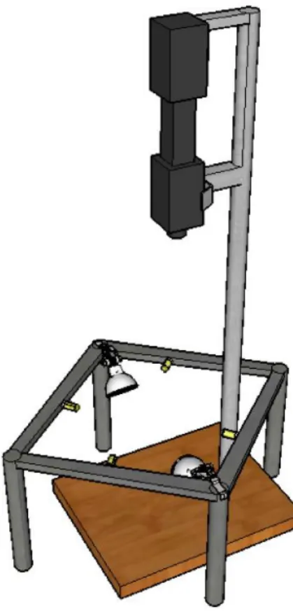
Figure 1 illustrates the experimental setup assembled for the hyperspectral image acquisition.
Source: Silva et al., 2016: para. 7.
Figure 1 – Experimental setup for hyperspectral image acquisition
Reflectance is the quotient between the intensity of the light reflected by an object and the light that illuminates that object, being a function of the light wavelength – these reflectance and absorption patterns across wavelengths can uniquely identify chemical compounds and,
16 unlike transmittance and interactance mode, it’s possible to perform the imaging without requiring contact between the spectrometer/camera and the sample.
For some position 𝑥, and at wavelength , the reflectance 𝑅 can be expressed as:
𝑅(𝑥, 𝜆) = 𝐺𝐼(𝑥, 𝜆) − 𝐷𝐼(𝑥, 𝜆) 𝑆𝐼(𝑥, 𝜆 ) − 𝐷𝐼(𝑥, 𝜆)
Equation 1 – Expressing reflectance as a function of some position and wavelength
Where 𝐺𝐼 is the intensity of light coming from the grape, 𝑆𝐼 is the intensity of light coming from the Spectralon and 𝐷𝐼 is the dark current signal, which is electronic noise – this value is measured with the hyperspectral camera lens covered and it must be subtracted from the grape and the Spectralon signal because it’s independent of the object being imaged and would distort the calculated reflectance values.
In order to achieve a reduction in measurement noise, 32 hyperspectral images were captured in each grape berry, from six grape berries and for three berry rotations – to create a single reflectance spectrum, all berries’ points were averaged over the spatial dimension and rotation. The reflectance measurement was done along the berry “equator” with the pedicel as the pole and the final spectrum was normalized to reduce the noise in the measured light intensities cause by the grape berry size and curvature: the normalization was performed subtracting from each spectrum its minimum values and dividing by the difference between the minimum and maximum values (Gomes et al., 2014b).
Graph 1 shows the final result for the reflectance measurements on the TF 2012 samples. Appendix J contains the results of the reflectance measurements for the remaining varieties and vintages of wine grape berries.
17
Graph 1 – Reflectance measurements for the TF 2012 samples
3.3. Data Pre-Processing
Prior to using the reflectance measurements as an input to the prediction models, it’s important to study the possible effects of different pre-processing methods that intend to transform the data to a form more suited for analysis by the machine learning algorithms. In this context, the Standard Normal Variate (SNV) Transformation (Fadock, 2011), Derivatives (Arana et al., 2005; Larraín et al., 2008), Multiplicative Scatter Correction (MSC) (Herrera et
al., 2003) and the Savitzky-Golay Filter (Herrera et al., 2003) arise as possible choices for
testing, since they are frequently used in spectroscopic measurements for chemical analysis of grapes - however, some authors claim that the use of pre-processing methods is actually detrimental to the final results, with published results by the aforementioned authors questioning the positive effects of Derivatives, MSC or SNV Transformation when applied to chemometric data. In this work, the author chose to implement the Savitzky-Golay Filter for the purpose of smoothing the data and the SNV Transformation to correct scatter and study its effects when compared to a model without any pre-processing methods applied to the reflectance measurements.
As in Savitzky and Golay (1964), the Savitzky-Golay Filter is a technique that attempts to “smooth” the data, that is, to increase the signal-to-noise ratio without distorting the signal. The authors found that a “least squares calculation, may be carried out in the computer by convolution of the data points with properly chosen sets of integers” (idem, p. 1627), without additional computational complexity – in the general case of a group of 𝐶 values representing
18 any set of convolutional integers, the mathematical description of the convolution process, with an associated normalizing or scaling factor, is:
𝑌𝑗∗= ∑ 𝐶𝑖𝑌𝑗+𝑖
𝑖=𝑚 𝑖= −𝑚
𝑁
Equation 2 – Description of the convolution process in a general case
With the index 𝑗 representing the running index of the ordinate data in the original data table and 𝑁 the normalizing factor. This calculation follows a common criterion to the best fit of least squares, with “the sole function of the computer is to act as a filter to smooth the noise fluctuations and hopefully to introduce no distortions into the recorded data” (idem, p. 1629). Graph 2 shows the reflectance measurements of the TF 2012 samples and the reflectance measurements of the TF 2012 samples after applying a Savitzky-Golay Filter with a frame length of 512nm and a third-degreed polynomial order, side-by-side to ease a comparison:
Graph 2 – Reflectance measurements for the Touriga Franca 2012 samples; a) Original; b) After applying the Savitzky-Golay Filter
The smoothing and noise reduction of the reflectance measurements is easily observable in Graph 2, especially in the 0-100 and 700-900nm wavelength regions, meaning that the least squares found an apparent good fit to the data.
19 The SNV transformation, as in Barnes, Dhanoa and Lister is a “mathematical transformation of the log (1
𝑅) spectra by calculation of the standard normal variation at each
wavelength […] removes slope variation on an individual sample basis by the use of the following calculation” (1989, p. 772):
𝑆𝑁𝑉(1−𝑊)= (𝑦1−𝑊− 𝑦̅) √∑(𝑦(1−𝑊)− 𝑦̅)2
𝑛 − 1
Equation 3 – Calculation of the standard normal variation at each wavelength W
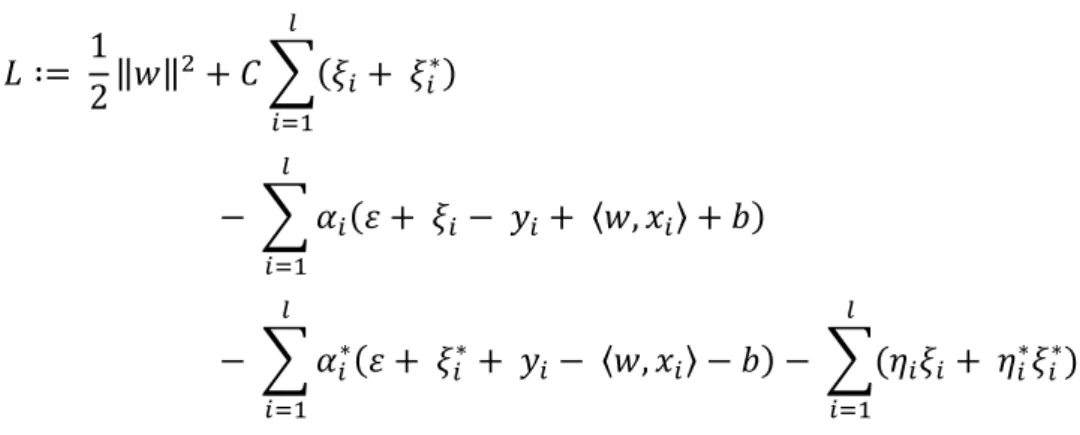
Where 𝑆𝑁𝑉(1−𝑊) are the individual standard normal variations for 𝑊 wavelengths, 𝑦 is the 𝑊-wavelength log (1
𝑅) values, and 𝑦̅ is the mean of the 𝑊-wavelength log ( 1
𝑅) values. This
calculation intends to effectively remove the multiplicative interferences of particle size and scatter, since there is a high degree of collinearity between data points in the log (1
𝑅) spectra,
which is a function to some extent of scatter and variable path length (idem). Graph 3 shows the reflectance measurements of the TF 2012 samples, the reflectance measurements of the TF 2012 samples after applying the described Savitzky-Golay Filter and the reflectance measurements after applying the SNV transformation to the data (applied to the original reflectance measurements), side-by-side to ease a comparison.
Graph 3 – Reflectance measurements for the TF 2012 samples; a) Original; b) After applying the Savitzky-Golay Filter; c) After applying the SNV transformation
20 Observing Graph 3, it’s noticeable that the range of reflectance values is different and that some of the graph peeks, either minimum or maximum, have a slightly different representation, possibly meaning that some interference due to scatter or particle size was removed in those regions.
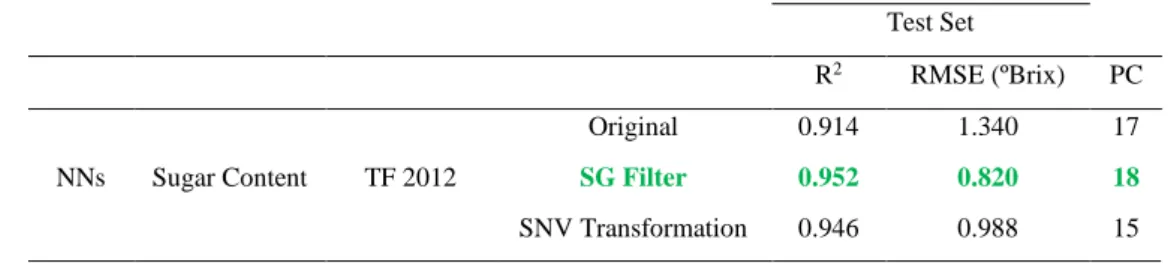
Table 5 contains the test set results obtained with a prediction model with the application of 10-fold cross-validation, PCA and NNs trained via the Levenberg-Marquardt algorithm and random initialization of the weights and bias (methods covered further in this chapter) for the estimation of sugar content on TF 2012 samples, to compare the different pre-processing methods.
Table 5 – Results obtained for the prediction of sugar content on TF 2012 samples with different pre-processing methods Test Set R2 RMSE (ºBrix) PC NNs Sugar Content TF 2012 Original 0.914 1.340 17 SG Filter 0.952 0.820 18 SNV Transformation 0.946 0.988 15
PC: Principal Components used. SG: Savitzky-Golay. SNV: Standard Normal Variate.
These results show that, for this particular test, a pre-processing step with the Savitzky-Golay filter is the best choice, since it’s the setup with the least Root Mean Squared Error (RMSE) and the best Coefficient of Determination (R2). For effects of this work, the author chose to include the Savitzky-Golay Filter in the pre-processing step since it lowers the prediction errors seemingly without adding complexity to the model (similar number of principal components used in all pre-processing methods – further analysis regarding this topic is presented in Chapter IV): however, further investigation should be conducted, since the study of different pre-processing methods and its effects aren’t the main objective of this work and there’s a wide variety of methods and testing setups that could have been used.
To finish the data pre-processing step two widely used operations, mean-centering and auto-scaling, as in Bro and Smilde were employed to the data matrix. “Centering is performed to make interval-scale data behave as ratio-scale data, which is the type of data assumed in most multivariate models” (2003, p. 19) and this operation should allow a “reduced rank of the
21 model”, an “increased fit to the data” and the “avoidance of numerical problems” (idem, ibidem). The mean-centering operation can be described by the equation below:
𝑀𝐶(𝑦) = 𝑦 − 𝑦̅
Equation 4 – Mean-centering operation on a dataset 𝒚
Where 𝑦 represents the original data and 𝑦̅ the vector with the mean of the dataset. As for scaling, as in Bro and Smilde, this operation is used to adjust for scale differences and to accommodate for heteroscedasticity (sub-populations with different variabilities), which is a very common concern in regression and variance analysis – in this work, the auto-scaling method was applied to let the variance of each variable be identical initially, so that the “subsequent fitting of a model is performed so as to describe as much systematic variation as possible […] every variable has the same initial opportunity of entering the model” (2003, p. 24). The equation below describes the auto-scaling operation:
𝑋𝑓= 𝑋 − 𝑋̅ 𝜎(𝑋)
Equation 5 – Auto-scaling operation on a dataset 𝑿
Where 𝑋 is the original data, 𝑋̿ the vector with the mean of the dataset and 𝜎(𝑋) the vector with the standard deviation of the dataset.
3.4. Dimensionality Reduction
The major disadvantage of the hyperspectral imaging technique is the dimensionality of the reflectance spectra, since the resulting matrix has a dimensionality equal to the number of spectral channels measured by the hyperspectral camera (namely, 1040). The difficulties in processing such large multivariate datasets are noticeable and, in order to obtain the maximum performance of the machine learning algorithms employed, a significant reduction of the size of its input is strictly necessary – for this work, a Principal Component Analysis (PCA) was implemented.
22 As in Wold, Esbensen and Geladi
“PCA provides an approximation of a data table, a data matrix, 𝑋, in terms of the product of two small matrices 𝑇 and 𝑃′ that captures the essential data patterns of 𝑋, providing the means to significantly reduce the size of a dataset without losing variability in the data. Plotting the columns of 𝑇 gives a picture of the dominant “object patterns” of 𝑋 and, analogously, plotting the rows of 𝑃′ show the complementary «variable patterns»” (1987, p. 37).
The columns in 𝑇 are called score vectors and the rows in 𝑃′ are called loading vectors, while the deviations between projections and the original coordinates are termed the residuals, collected in the matrix 𝐸 (idem). The equation below shows the PCA in matrix form as a least squares model of:
𝑋 = 1𝑥̅ + 𝑇𝑃′+ 𝐸
Equation 6 – PCA in matrix form
Here the mean vector 𝑥̅ is explicitly included in the model formulation.
“A basic assumption in the use of PCA is that the score and loading vectors corresponding to the largest eigenvalues contain the most useful information relating to the specific problem, and that the remaining ones mainly comprise noise: therefore, these vectors are usually written in order of descending eigenvalues” (Wold, Esbensen and Geladi, 1987, p. 42).
Graph 4 shows a scree plot (plot of the eigenvalues in descending order) of the PCA implementation for the TF 2012 reflectance measurements:
23 In general cases, the number of factors retained for analysis are those with eigenvalues over 1: as seen in the graph, two principal components describe most of the variance in the population (roughly 96.7% of all the variance in a cumulative sum), while the other factors, as stated above, would mainly comprise noise – however, in this case this assumption might not be true due to the highly complex chemical interactions present in the samples that have an impact on the reflectance measurements – there isn’t a clear answer to how many factors should be retained for analysis (only general rules of thumb, like the scree plot analysis) and in this work, every model was tested using between 1 and 50 principal components, saving the best result (further analysis is shown in Chapter IV).
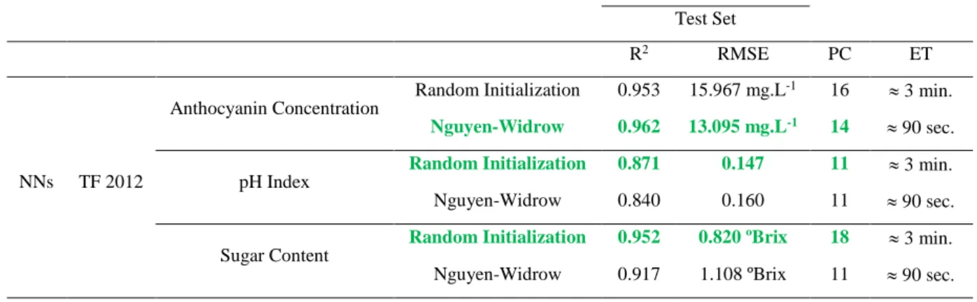
Table 6 contains the test results obtained with a prediction model with the application of the Savitzky-Golay Filter, 10-fold cross-validation and NNs trained via the Levenberg-Marquardt algorithm and random initialization of the weights and bias (k-Fold Cross-Validation and NNs will be covered further in this chapter) for the estimation of sugar content on TF 2012 samples, to compare the use of the PCA before applying a machine learning algorithm on the “raw” reflectance measurements.
Table 6 – Results obtained for the prediction of sugar content on TF 2012 samples with and without the application of a PCA
Test Set
R2 RMSE (ºBrix) PC
NNs Sugar Content TF 2012 Principal Component Analysis 0.952 0.820 18
Original * 0.839 1.678 -
PC: Principal Components used. *With Savitzky-Golay Filter.
The results presented show that, for this test setup, the NN model takes great benefit from a dimensionality reduction step, specifically with the implementation of a PCA, achieving a significantly better R2 and a lowest RMSE – additionally, the computational cost when using the PCA before employing the machine learning algorithm is greatly reduced (which is expected, since the algorithm works with a significantly smaller set of inputs). For this work, the author chose to include the PCA as a dimensionality reduction step for every prediction model: however, there is a wide variety of dimensionality reduction methods that can be tested and further investigation in this topic should be conducted.
24 3.5. Model Validation
Model validation (or model selection, model evaluation)
“can be understood primarily as a way of measuring the predictive performance of a statistical model, since high values of R2 don’t necessarily mean a good fit – the model may have
introduced too many degrees of freedom and inflate this statistics by overfitting the data, which means that predictions on new data will usually get worse as higher order terms are added. One way to measure the predictive ability of a model is to test it on a set of data not used in the estimation, a «validation or test set», instead of the «training set» used for estimation: however, there is often not enough data to allow for some of it to be kept back for testing” (Hyndman, 2010).
In this context, cross-validation and bootstrapping methods arise as a viable choice to improve the models’ generalization capacity without adding more samples to a dataset. In this work, the k-Fold Cross-Validation, Monte-Carlo Cross-Validation and Bootstrap methods were implemented and their efficiency compared as to choose the most adequate method to compose the predictive model; their description is found below, as in Lendasse, Wertz and Verleysen (2003).
The consecutive steps of the Monte-Carlo Cross-Validation are:
1. One randomly draws without replacement some elements of the dataset 𝑋; these elements form a new learning dataset 𝑋𝑙𝑒𝑎𝑟𝑛. The remaining elements of 𝑋 form the validation set 𝑋𝑣𝑎𝑙 (see Figure 2).
Source: Remesan & Mathew, 2014: 64
Figure 2 – Data splitting in the random sub-sampling (Monte-Carlo) approach
2. The training of the model 𝑔 is done using 𝑋𝑙𝑒𝑎𝑟𝑛 and the error 𝐸𝑘(𝑔) is calculated