Analysis of snow bidirectional reflectance from ARCTAS spring-2008 campaign

(1)

ACPD

9, 21993–22040, 2009

Analysis of snow bidirectional reflectance from

ARCTAS

A. Lyapustin et al.

Title Page

Abstract Introduction

Conclusions References

Tables Figures

◭ ◮

Back Close

Full Screen / Esc

Printer-friendly Version

Interactive Discussion Atmos. Chem. Phys. Discuss., 9, 21993–22040, 2009

www.atmos-chem-phys-discuss.net/9/21993/2009/ © Author(s) 2009. This work is distributed under the Creative Commons Attribution 3.0 License.

Atmospheric Chemistry and Physics Discussions

This discussion paper is/has been under review for the journalAtmospheric Chemistry and Physics (ACP). Please refer to the corresponding final paper inACPif available.

Analysis of snow bidirectional reflectance

from ARCTAS spring-2008 campaign

A. Lyapustin1,2, C. K. Gatebe1,2, R. Kahn2, R. Brandt3, J. Redemann4, P. Russell5, M. D. King6, C. A. Pedersen7, S. Gerland7, R. Poudyal8,2, A. Marshak2, Y. Wang1,2, C. Schaaf9, D. Hall2, and A. Kokhanovsky10

1

University of Maryland Baltimore County, Baltimore, MD, USA

2

NASA Goddard Space Flight Center, Greenbelt, MD, USA

3

University of Washington, Seattle, Washington, USA

4

Bay Area Environmental Research Institute (BAERI), Sonoma, CA USA

5

NASA Ames Research Center, Moffett Field, CA, USA

6

University of Colorado, Boulder, CO, USA

7

Norwegian Polar Institute, 9296 Tromsø, Norway

8

Science Systems and Applications, Inc., Lanham, MD, USA

9

Boston University, Boston, USA

10

Institute of Environmental Physics, University of Bremen, 28359 Bremen, Germany

Received: 16 September 2009 – Accepted: 30 September 2009 – Published: 20 October 2009 Correspondence to: A. Lyapustin ([email protected])

(2)

ACPD

9, 21993–22040, 2009

ARCTAS

A. Lyapustin et al.

Title Page

Tables Figures

◭ ◮

Back Close

Full Screen / Esc

Interactive Discussion

Abstract

The spring 2008 Arctic Research of the Composition of the Troposphere from Aircraft and Satellites (ARCTAS) experiment was one of the major intensive field campaigns of the International Polar Year, aimed at detailed characterization of atmospheric physi-cal and chemiphysi-cal processes in the Arctic region. Part of this campaign was a unique 5

snow bidirectional reflectance experiment on the NASA P-3B aircraft conducted on 7 and 15 April by the Cloud Absorption Radiometer (CAR) jointly with airborne Ames Airborne Tracking Sunphotometer (AATS) and ground-based Aerosol Robotic Network (AERONET) sunphotometers. The CAR data were atmospherically corrected to derive snow bidirectional reflectance at high 1◦angular resolution in view zenith and azimuthal 10

angles along with surface albedo. The derived albedo was generally in good agreement with ground albedo measurements collected on 15 April. The CAR snow bidirectional reflectance factor (BRF) was used to study the accuracy of analytical Ross-Thick Li-Sparse (RTLS), Modified Rahman-Pinty-Verstraete (MRPV) and Asymptotic Analytical Radiative Transfer (AART) BRF models. Except for the glint region (azimuthal an-15

glesϕ<40◦), the best fit MRPV and RTLS models fit snow BRF to within _±0.05. The plane-parallel radiative transfer (PPRT) solution was also analyzed with the models of spheres, spheroids, randomly oriented fractal crystals, and with a synthetic phase func-tion. The latter merged the model of spheroids for the forward scattering angles with the fractal model in the backscattering direction. The PPRT solution with synthetic phase 20

function provided the best fit to measured BRF in the full range of angles. Regard-less of the snow grain shape, the PPRT model significantly over-/underestimated snow BRF in the glint/backscattering regions, respectively, which agrees with other studies. To improve agreement with the experiment, we introduced a model of macroscopic snow surface roughness by averaging the PPRT solution over the slope distribution 25

(3)

ACPD

9, 21993–22040, 2009

ARCTAS

A. Lyapustin et al.

Title Page

Tables Figures

◭ ◮

Back Close

Full Screen / Esc

Interactive Discussion at view zenith angles below 55–60◦covering the practically important range for remote

sensing applications, and includes both glint and backscattering directions.

1 Introduction

Due to its high reflectance, snow is one of the key factors defining the surface radiative budget in polar regions and affecting global climate of the Earth. The albedo of thick 5

snowpack is governed primarily by the snow grain size and level of impurities, such as soot or dust, deposited from the atmosphere. Monitoring snow properties from space requires an accurate knowledge of its bidirectional reflectance factor (BRF) (Stroeve and Nolin, 2002; Stroeve et al., 2005; Stamnes et al., 2007; Scambos et al., 2007; Painter et al., 2009; Lyapustin et al., 2009). Accurate modeling of snow reflectance 10

is equally important for atmospheric remote sensing of cloud properties and vital for aerosol retrievals over snow-covered regions, which presently remains a largely unre-solved problem.

Beginning with the classic work of Wiscombe and Warren (1980), snow reflectance has been studied extensively using a plane-parallel radiative transfer model. The ac-15

cumulated body of measurements and modeling e_fforts unites in understanding that the bidirectional reflectance of snow is less anisotropic than predicted by the RT model (e.g., Warren et al., 1998; Painter and Dozier, 2004; Hudson et al., 2006; Hudson and Warren, 2007). The main errors appear around the principal plane, where the model significantly overestimates reflectance in the forward scattering angles and un-20

derestimates it in backscattering directions. Because of the apparent nonsphericity of snow grains, a number of studies investigated the effect of the snow particle shape on the modeled reflectance (Mishchenko et al., 1999; Xie et al., 2006; Jin et al., 2008). Yang and Liou (1998), Kokhanovsky and Zege (2004), and Jin et al. the (2008) found that using the nonspherical model of snow grains improves agreement with measure-25

(4)

ACPD

9, 21993–22040, 2009

ARCTAS

A. Lyapustin et al.

Title Page

Tables Figures

◭ ◮

Back Close

Full Screen / Esc

Interactive Discussion over Antarctica (Hudson et al., 2006). Although microscopic roughness (with scale

much less than the grain size) smoothed the di_fference, the best theoretical predictions still significantly overestimate the tower snow reflectance in the forward scattering an-gles and underestimate it in the backscattering region. Overall, the authors achieved agreement between modeled radiance and tower measurements within_±10% for view 5

zenith angles ≤60◦, with the above-mentioned asymmetry between the forward and backscattering directions. These studies help clarify the point that the microphysical variability alone cannot fully capture all the features of snow reflectance, and macro-scopic (∼10 cm) effects of non-flat snow surfaces and shadows need to be incorporated into the model to achieve closure with measured snow BRF, even at the tower-scale 10

footprint, not to mention the satellite footprint. Hudson and Warren (2007) have demon-strated the effect of snow surface roughness by contrasting snow reflectance under clear skies with that from clouds over the snow at different view zenith angles. Nolin et al. (2002) used multi-angle MISR data to characterize roughness of sea ice and ice sheets over Greenland and Antarctica. A study by Leroux and Fily (1998) showed that 15

modeling the effect of sastrugi improved the agreement with snow BRF measurements over Antarctica.

In this work, we study the effect of macroscopic surface roughness, including the slope distribution of reflecting facets and shadows cast by sastrugi, using a simple model. We also study the accuracy of the common analytical BRF models used in oper-20

ational satellite data processing, including the reciprocal Ross-Thick Li-Sparse (RTLS, Lucht et al., 2000), Modified Rahman-Pinty-Verstraete (MRPV, Martonchik et al., 1998), and Asymptotic Analytical Radiative Transfer (AART, Kokhanovsky and Zege, 2004) models. In parallel, we evaluate the atmospheric correction error over snow due to the Lambertian assumption, which is the basis of MODIS operational land processing 25

(Vermote and Kotchenova, 2008).

(5)

ACPD

9, 21993–22040, 2009

ARCTAS

A. Lyapustin et al.

Title Page

Tables Figures

◭ ◮

Back Close

Full Screen / Esc

Interactive Discussion aerosol measurements from the Aerosol Robotic Network (AERONET, Holben et al.,

1998) and data from the Ames Airborne Tracking Sunphotometer (AATS, Russell et al., 2005, 2007) to derive snow BRF. CAR provides comprehensive spectral coverage from the UV through shortwave infrared spectral region, and has unprecedented angular resolution for an airborne sensor of 1◦ in zenith and azimuthal angles. Several repre-5

sentative experiments were conducted at Barrow, Alaska over Elson Lagoon. Different flight altitudes allowed us to test the atmospheric correction algorithm and get insight into snow spatial homogeneity at scales of ∼0.2–2 km. The atmospheric correction algorithm is independently evaluated against surface measurements of snow albedo.

This paper is organized as follows: Section 2 provides a brief description of the NASA 10

P-3B aircraft flights, focusing on CAR measurements, and Sect. 3 describes the ground albedo experiment. The atmospheric correction algorithm is described in Sect. 4, along with its evaluation. Based on derived snow BRF, Sect. 5 examines analytical BRF models. Finally, macroscopic surface roughness is explored in Sect. 6, followed by Conclusions. The analytical BRF models and the model of surface roughness are 15

described in the Appendices.

2 Description of experiments

The ARCTAS Spring campaign was conducted between 1–21 April 2008, with the aim of studying physical and chemical processes in the Arctic atmosphere and related sur-face phenomena, as part of the International Polar Year. NASA deployed two aircraft 20

from Fairbanks, Alaska, the DC-8, instrumented primarily for atmospheric chemical sampling and the P-3B, which carried a payload, including the CAR and AATS instru-ments, designed to study aerosols and the radiation environment (Jacob et al., 2009). A third NASA aircraft, the B200, was stationed at Barrow, Alaska, and carried the NASA Langley High-Spectral-Resolution Lidar (HSRL; Hair et al., 2008). In addition, a num-25

(6)

ACPD

9, 21993–22040, 2009

ARCTAS

A. Lyapustin et al.

Title Page

Tables Figures

◭ ◮

Back Close

Full Screen / Esc

Interactive Discussion one at Barrow and one at Eureka, Canada.

The ARCTAS directional snow reflectance experiment addressed multiple objectives, as the albedo and the snow reflectance angular variation are critical for surface charac-terization, energy balance calculations, and the remote sensing of atmospheric proper-ties, including aerosol amount and type. For this experiment, we collected concurrent 5

observations of the snow-covered surface from platforms at multiple levels. The suite of measurements included ground-based Analytic Spectral Device (ASD) FieldSpec radiometer observations and direct snow samples, airborne instrument data, including CAR and AATS remote sensing from the P-3B, and near-coincident observations from the NASA Earth Observing System’s Terra satellite Multi-angle Imaging SpectroRa-10

diometer (MISR) and MODerate-resolution Imaging Spectroradiometer (MODIS). The primary target site for this experiment was Elson Lagoon (71.3◦N, 156.4◦W), near Bar-row, Alaska, which was studied by the P-3B payload on 7 and 15 April. The HSRL joined the P-3B on 7 April, and concurrent surface measurement took place the week of 15 April. Other sets of measurements over snow surface was made with the P-3B 15

instruments on 8 April near Eureka, Canada (80.5◦N, 90.2◦W) and on 9 April near Axel Heiberg Island, Canada (79.9◦N, 100.9◦W). The present study focuses on the Elson Lagoon events.

3 Albedo measurements at the surface

A site was selected 10 km east (upwind) of Barrow, Alaska, on Elson Lagoon. This 20

lagoon is a protected arm of the Beaufort Sea. The surface consisted of flat land-fast first-year sea ice of thickness_∼1.5 m, covered with 25–40 cm of snow, with a density of 0.35 g cm−3. The snow surface roughness was in the form of small sastrugi, with a typical height_∼5 cm and spacing _∼1 m (Fig. 1). The lagoon is a homogeneous area large enough to ensure a uniform representative footprint in the field of view of the CAR 25

from the P-3B airplane.

(7)

manu-ACPD

9, 21993–22040, 2009

ARCTAS

A. Lyapustin et al.

Title Page

Tables Figures

◭ ◮

Back Close

Full Screen / Esc

Interactive Discussion factured by Analytical Spectral Devices, Inc. (ASD). The instrument records radiance

every 1 nm from 350 to 2500 nm wavelength, with 3- to 30-nm spectral resolution (full width at half maximum). The instrument is described by Kindel et al. (2001). At Barrow, two of these ASD instruments were deployed, one from the University of Washington (UW) and the other from the Norwegian Polar Institute (NPI). A “cosine collector” (re-5

ceiving radiation from a hemisphere, 2πsr) is supported by a 1.6-m rod, mounted on a tripod. The cosine collector is designed to accept incident radiation with equal effi -ciency from any angle in the hemisphere; if it does so then the signal produced as the collector plane is rotated relative to a point source is proportional to the cosine of the incidence angle, because the projected area of the collector plane is proportional to the 10

cosine. Spectral albedo is usually measured more accurately under an overcast sky because the radiation from both upward and downward hemispheres is diffuse, so er-rors in leveling the instrument, deviations from cosine response, and non-horizontality of the surface all cause much smaller errors than under direct-beam incidence.

The rod has bubble levels at both ends, so the cosine collector can be rotated to 15

view the upward and downward hemispheres alternately. The light received by the cosine collector is directed by a fiber-optics guide to the ASD detector. Although the two radiometers were identical, their cosine collectors were not. The cosine collectors were calibrated as in Grenfell et al. (1994). The UW instrument had better cosine-response than the NPI instrument at infrared wavelengths, and the reverse was true at 20

visible wavelengths; this affects our selection of data below.

Under overcast skies with diffuse incidence, the cosine collector, support rod, tripod, radiometer box, computer, and sled all intercept some of the downward solar radiation that would reach the snow surface below the cosine collector if the instrument were not there. A “shadowing correction” was applied to the albedo measurements. For diffuse 25

incidence the shadowing correction was estimated by geometric analysis as 1.7% for the UW instrument and 0.6% for the NPI instrument. For direct incidence with low sun, the shadowing correction is smaller.

(8)

ACPD

9, 21993–22040, 2009

ARCTAS

A. Lyapustin et al.

Title Page

Tables Figures

◭ ◮

Back Close

Full Screen / Esc

Interactive Discussion overcast skies; on one of those days, 15 April, simultaneous measurements were made

with the CAR from the NASA P-3B aircraft flying over Elson Lagoon. The surface air temperature during the surface albedo experiments was in the range ₋14 to ₋21◦C throughout 14–17 April. On the 19th it was warmer,₋1.3◦C.

3.1 Measurements on 15 April

5

Fresh snow had fallen on 14 April with minimal redistribution by the wind. Albedo was measured at five sites near the center of our designated clean area along a westerly track at 50-m intervals. The variation in measured albedo at a given site was significant, due to slight leveling errors in positioning the cosine collector.

A leveling-error correction was applied as a spectrally-constant scale factor, chosen 10

so as to adjust the 490-nm albedo to equal that measured on 19 April with diffuse illumination (overcast cloud). The measurements on 19 April were not a_ffected by leveling errors because the incident of radiation was diffuse, and the high albedo at 490 nm is insensitive to grain size variation (Wiscombe and Warren, 1980, Fig. 8a). Furthermore, the solar zenith angle during the 15 April measurements was_∼60◦, which 15

is close to the effective incidence angle of diffuse irradiance, so the effect of zenith-angle difference on albedo of the two days should be negligible, particularly at 490 nm where albedo is insensitive to zenith angle (Wiscombe and Warren, 1980, Fig. 11).

A correction was applied for the radiometer and support shadows, which blocked a small portion of the downward looking field-of-view. Due to differences in cosine col-20

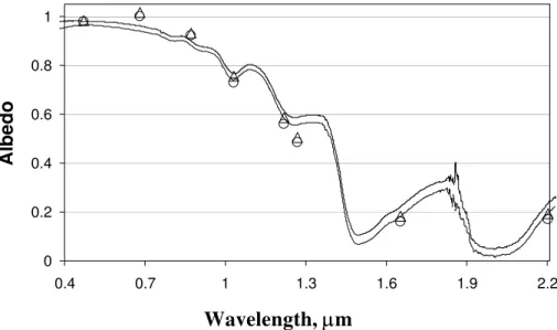
lector design, the NPI ASD was more accurate for wavelength below_∼1 µm, whereas the UW ASD provided a better signal/noise ratio beyond∼1 µm. For this reason the UW albedos were scaled slightly to match the NPI albedo in the 800–850 nm band where both instruments performed well. The final result (Fig. 2) is a combination of the NPI albedo at UV and visible wavelengths and the UW albedo in the near-infrared. 25

(9)

ACPD

9, 21993–22040, 2009

ARCTAS

A. Lyapustin et al.

Title Page

Tables Figures

◭ ◮

Back Close

Full Screen / Esc

Interactive Discussion final reported albedo. The error envelope in Fig. 2 includes variation between sites,

estimated error in the shadowing correction and error in assigning the 490-nm albedo.

4 Processing CAR data

4.1 Atmospheric correction algorithm

To process CAR data over snow, a specialized atmospheric correction algorithm has 5

been developed. It is based on an accurate semianalytical expression for the atmo-spheric radiance derived with the Green’s function method (Lyapustin and Knyazikhin, 2001; Lyapustin and Wang, 2005). When used with the RTLS model (see Appendix A), this solution makes it possible to express upward reflectance at an arbitrary altitudez

in the atmosphere as an explicit function of RTLS model parametersK={kL, kG, kV}: 10

R(z; µ0,µ, ϕ) =RD(z; µ0,µ, ϕ)+kLFL(z; µ0,µ)+kGFG(z; µ0,µ, ϕ)

+kVFV(z; µ0,µ, ϕ)+Rnl(z; µ0,µ), (1) whereRD is the atmospheric (path) reflectance,Fk (k=L, G, V) are functions of view geometry and atmospheric properties, µ0and µ are cosines of the solar and view zenith angles, respectively, andϕis the relative azimuth angle. FunctionsFkhave a weak de-15

pendence on surface reflectance through a multiple reflection factor,α=(1−q(µ0)s)− 1

, whereq is surface albedo andsis spherical albedo of the atmosphere. Rnl is a small term nonlinear in surface reflectance.

The quasi-linear form of Eq. (1) leads to a very efficient iterative minimization algo-rithm for the root-mean-square error for three parameters of RTLS modelK:

20

RMSE=X

j

(r_j(n)−F_jLkL(n)−F_jVkV(n)−F_jGkG(n))2=min {K_} ,

where

(10)

ACPD

9, 21993–22040, 2009

ARCTAS

A. Lyapustin et al.

Title Page Abstract Introduction Conclusions References Tables Figures ◭ ◮ ◭ ◮ Back Close

Full Screen / Esc

Interactive Discussion In this expression, R is a measured CAR reflectance, the index j denotes different

CAR view angles, and n is the iteration number. Although it is not shown explicitly, functionsFk are also updated every iteration, according to current value of parameter

α. Equation (2) provides an explicit least-squares solution for coefficientsK:

K(n)=A−1b(n), (3) 5 where A=        P

(F_jL)2 P

j

F_jGF_jL P

j

F_jVF_jL

P

j

F_jGF_jL P

j

(F_jG)2 P

j

F_jVF_jG

P

j

F_jVF_jLP

j

F_jVF_jG P

j

(F_jV)2       

, b(n)=        P j

r_j(n)F_jL

P

j

r_j(n)F_jG

P

j

r_j(n)F_jV

       .

In the first iteration, the non-linear term is computed for an assumed spectrally depen-dent albedo, for exampleq(0)(vis)₌0.6, orq(0)(2.2 µm)₌0.05. Convergence is achieved in 4–5 iterations over bright snow in the CAR blue band (0.48 µm), and it takes fewer 10

iterations at longer wavelengths where snow is less reflective.

Once RTLS coe_fficients are computed, the di_ffuse component of the surface-reflected signal (RDif) is calculated at the altitude z of P-3B flight, and the snow bidi-rectional reflectance factorρ, representing specific measurements, is computed from the direct reflected term. For this purpose, we single-out the direct term and re-write 15

Eq. (1) as follows:

R(z; µ0,µ, ϕ)=RD(z; µ0,µ, ϕ)+RDif(z;K; µ0,µ, ϕ)+ρ(µ0,µ, ϕ)e−τ0/µ0e−(τ0−τ(z))/|µ|.(4) Here, τ₀ is the column optical depth through the atmosphere at the wavelength of interest. Finally, once the snow BRF is computed, the best-fit parameters of the MRPV and AART models are retrieved and the rmse is evaluated. The MRPV parameters 20

(11)

ACPD

9, 21993–22040, 2009

ARCTAS

A. Lyapustin et al.

Title Page

Tables Figures

◭ ◮

Back Close

Full Screen / Esc

Interactive Discussion the SHARM code (Lyapustin and Wang, 2005). Assuming all the ozone is located

above the aircraft, the CAR data are preliminarily corrected for ozone absorption along the solar path.

4.2 Ancillary parameters

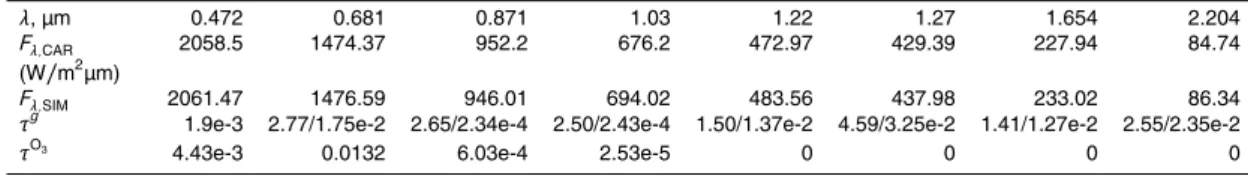
Table 1 lists the CAR spectral bands, the in-band solar irradiance used to convert digital 5

numbers into reflectance units, and the assumed optical thickness of column gaseous absorption. The latter includes 0.4 cm column water vapor that is close to the AATS above airplane value at the lowest flight altitude (Schmid et al., 2003; Livingston et al., 2008) and to the AERONET column measurement at the Barrow site during these experiments. The monochromatic gaseous absorption, τg(λ), is computed using the 10

equation: exp{−τg}=

Z

∆λ

F_λexp{−τg(λ)}h_λd λ.

Z

∆λ

F_λh_λd λ , (5)

whereh_λ is the CAR relative spectral response function, andF_λis the exoatmospheric spectral solar irradiance. The optical thickness of absorbing gases is calculated for a carbon dioxide concentration of 340 ppm, and other gas concentrations correspond-15

ing to the sub-Arctic Winter atmospheric model (Kneizys et al., 1996). The calculations included absorption of six major atmospheric gases (H2O, CO2, CH4, NO2, CO, N2O) with line parameters from the HITRAN-2000 (Rothman et al., 2003) database, using the Voigt spectral line shape and the Atmospheric Environmental Research continuum absorption model (Clough et al., 2005). Because of the water vapor, oxygen and other 20

(12)

ACPD

9, 21993–22040, 2009

ARCTAS

A. Lyapustin et al.

Title Page

Tables Figures

◭ ◮

Back Close

Full Screen / Esc

Interactive Discussion a given θ0, although it may introduce some view-angle dependent error on the light

path from the surface to the aircraft. This error, however, is small because the flights were at low altitude (0.2–1.7 km) and the gaseous absorption is low. Table 1 also lists the in-band optical thickness of ozone absorption for 380 DU that was observed over Barrow during 7–15 April by the Ozone Monitoring Instrument (OMI). To verify CAR 5

calibration in reflectance units, we provide irradianceFλ obtained by integrating data

from Solar Irradiance Monitor on SORCE (Harder et al., 2000) collected on 8 April. The aerosol optical thickness above the P-3B aircraft was measured by the AATS onboard the aircraft, and the total column aerosol optical thickness was acquired by the AERONET sunphotometer at Barrow. The column water vapor provided by AERONET 10

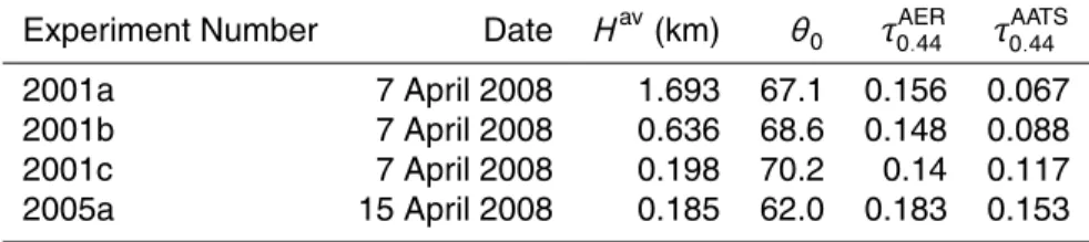
was low,_∼0.4 cm. Table 2 summarizes the P-3B flights with CAR measurements over snow, including dates, average height, solar zenith angle, and AERONET and AATS aerosol optical thickness.

4.3 Algorithm and CAR data analysis

Snow is the most reflective of the common land surface types, having an albedo close 15

to unity in the visible spectrum, and data analysis over pure snow raises accuracy stan-dards for the processing model as well as for sensor calibration accuracy. It may be mentioned in advance that CAR has provided excellent spectral BRF data for snow anisotropy analysis. However, we encountered a problem regarding the overall re-flectance magnitude at the red band (0.68 µm) in the experiment conducted on 7 April, 20

which is described and analyzed in this section.

The atmospheric correction algorithm developed here automatically computes sur-face albedo once the RTLS model parameters are found. The RTLS model approxi-mates snow BRF rather well, with standard deviation in the blue band below 3% relative to nadir. Forward computations with derived snow BRF reproduce the CAR measure-25

(13)

ACPD

9, 21993–22040, 2009

ARCTAS

A. Lyapustin et al.

Title Page

Tables Figures

◭ ◮

Back Close

Full Screen / Esc

Interactive Discussion on 15 April at lower solar zenith angle. These analyses support the conclusion that

the algorithm works correctly. However, the albedo derived for the CAR red band on 7 April was found to be slightly but systematically higher than unity, which violates energy conservation.

The derived spectral albedo was compared with surface albedo measurements col-5

lected on 15 April. Figure 2 shows the envelope of measured albedo from minimal to maximal values over the five sites; they are within about_∼2% in the visible bands. The triangles and circles show albedo derived at the CAR central wavelengths on 7 and 15 April, respectively. The overall agreement between CAR and ground albedo is good, especially given the possible snow inhomogeneity, and the difference between the CAR 10

footprint and the coverage of ground measurements. Except in the red (0.68 µm) and NIR (1.27 µm) bands, the retrievals are within or very close to the envelope of mea-sured albedo. In the red band, however, derived albedo is about 4–5% higher than the maximal measured value. It exceeds unity on 7 April (q=1.015) and is very close to unity (0.999) on 15 April.

15

We analyzed the main factors affecting the CAR red band results.

1) To exclude the possibility of error in the calibration conversion coefficients from radiance digital number (DN) counts to reflectance, the irradiance Fλ used in CAR

calibration was compared with data from the Solar Irradiance Monitor (Harder et al., 2000) integrated over the CAR spectral response (see Table 1). Although the use of 20

SIM irradiance reduces reflectance in the red band, the e_ffect is only about 0.1%. 2) Because of the relatively large solar zenith angle, it is important to accurately model absorption by well-mixed gases. The CAR red channel overlaps with the weak oxygen B-band, the main absorber in this channel apart from ozone. Our current mod-eling of absorption relies on the HITRAN-2000 edition. Although the new HITRAN-2008 25

(14)

ACPD

9, 21993–22040, 2009

ARCTAS

A. Lyapustin et al.

Title Page

Tables Figures

◭ ◮

Back Close

Full Screen / Esc

Interactive Discussion 3) Two algorithm-related factors were investigated as part of this analysis. First,

although CAR provides the full hemisphere of upward directions, the maximal view zenith angle (θ) in our processing is limited to about 75◦to conform to the limits of the plane-parallel radiative transfer model. To assess whether the upper θ limit impacts derived RTLS coe_fficients and albedo, θmax was varied from 60◦ to 85◦. The solution 5

was very stable, with maximal change below 0.2% in the blue band and negligible in the other bands. Second, the accuracy of the best-fit RTLS model is not uniform on the hemisphere of upward directions, and potentially, high outliers may bias the derived albedo. To investigate this factor, we added a separate albedo retrieval algorithm that does not depend on the model of surface BRF. It consists of three steps: in the first step, 10

CAR measured radiance is directly integrated using Simpson’s quadrature to obtain upward flux at the flight altitudez,

Fup(z; µ0)=µ0 2π

Z

0

d ϕ

0 Z

−1

µR(z; µ0,µ, ϕ)dµ. (6)

Next, this flux is extrapolated to the surface level,Fup(0; µ0)=F up

(z; µ0)

F_{T h}up(0;µ₀)

F_{T h}up(z;µ₀), where

F_{T h}up is a “theoretical” flux computed with the best-fit RTLS parameters and given an 15

atmospheric profile. Although individual “theoretical” fluxes at levelszandz=0 depend on parameters of the BRF model, this dependence disappears in the ratio. Finally, surface albedo is computed by dividing obtained reflected fluxFup(0; µ0) by the “theo-retical” incident fluxF_{T h}d n(0; µ0). We found that this approach generally decreases the albedo by 0.8% in the blue band, and by 0.5–0.2% at longer wavelengths, the di_ff er-20

ence diminishing with wavelength. This albedo reduction is taken into account in the data shown in Fig. 2.

(15)

ACPD

9, 21993–22040, 2009

ARCTAS

A. Lyapustin et al.

Title Page

Tables Figures

◭ ◮

Back Close

Full Screen / Esc

Interactive Discussion which may have an absolute uncertainty within 5%. Given this source of uncertainty,

the bias in the red band has yet to be explained, particularly in view of the absence of such a bias in the nearby blue band. Our analysis will continue with further investigation of issues related to the processing algorithm and absolute CAR calibration.

5 Bidirectional reflectance of snow

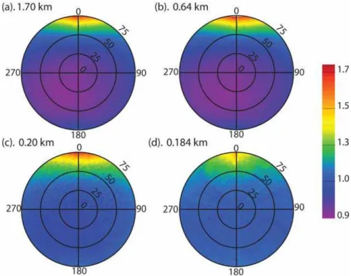
5

Figure 3 shows the derived snow BRF in the CAR red band. The first three images show results for 7 April from three different observing altitudes, 1.7, 0.64, and 0.2 km, and the last image shows retrievals for 15 April for measurements from 184 m altitude. The BRF has a very consistent pattern, with a shape dominated by two features – the increase of reflectance in the glint (forward scattering) direction, and a smaller 10

reflectance increase in the backscattering direction. The dark feature in the hotspot direction in the last two images (c and d) corresponds to the airplane shadow.

The radiometer scans different surface points while obtaining the total BRF. The CAR footprint decreases, and spatial resolution increases, at lower flight altitudes; the effect of surface inhomogeneity becomes clearly visible at altitudes of_∼0.2 km and below, on 15

both 7 and 15 April. Analysis of BRF at angles close to nadir, for example atθ<3◦, makes it possible to evaluate snow reflectance variability (inhomogeneity) as∼0.05 for flight altitudes above 0.6 km and_∼0.15–0.2 for 0.2 km altitude.

Snow BRFs remain close in the blue-NIR range, 0.47–0.87 µm. Although the imag-inary part of the ice refractive index increases with wavelength, it remains very low 20

in this spectral range, as does snow absorption. In these conditions, BRF is dom-inated by multiple scattering, and BRF anisotropy is low. At longer wavelengths, absorption becomes progressively more prominent, and as the magnitude of snow reflectance drops, reflectance anisotropy increases. This result is shown in Fig. 4, which shows the spectral dependence of snow BRF in the principal plane and in 25

(16)

ACPD

9, 21993–22040, 2009

ARCTAS

A. Lyapustin et al.

Title Page

Tables Figures

◭ ◮

Back Close

Full Screen / Esc

Interactive Discussion CAR signal and the retrieved BRF. Taking the ratio Ratio=ρ(θ=60◦)/ρ (θ=0◦) at

ϕ=0◦ in the principal plane as a measure of anisotropy, one can see the increase of anisotropy with wavelength quantitatively: ratio={1.44; 1.48; 1.69; 1.93; 1.99; 3.66; 3.7_} atλ={0.68; 0.87; 1.03; 1.22; 1.27; 1.65,2.2}. Here, we omitted the blue band because of the saturation problem.

5

The cross-plane (ϕ=90◦) reflectance increases systematically with the view zenith angle. Although anisotropy of reflectance is notably lower than in the principal plane, nonetheless snow reflectance is significantly non-Lambertian.

6 Analysis of MRPV and RTLS models

The RTLS and MRPV models (see Appendix A) are used in the MODIS (Schaaf et al., 10

2002) and MISR (Martonchik et al., 1998) land algorithms, respectively, including snow-covered surfaces. The accuracies of these models were studied experimentally over different land cover types (Privette et al., 1997; Bicheron and Leroy, 2000), however, we are not aware of such analysis over snow. The CAR dataset presents an excellent opportunity to perform an accuracy analysis over pure snow.

15

In order to remedy a possible bias in the CAR red band discussed in Sect. 4.3 and shown in Fig. 2, the derived BRF was renormalized by matching retrieved red band albedo with the mean value from ground-based measurements. This renormalization does not a_ffect the reflectance angular distribution. The retrieved and normalized snow BRF is used below to evaluate accuracy by the RTLS and MRPV models.

20

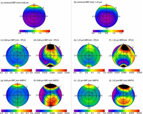
The results of the model analysis are shown in Fig. 5 for the red (0.67 µm) and NIR (1.22 µm) bands that are often used in snow property retrievals. The left image shows the retrieved BRF followed by images showing accuracy of the RTLS and MRPV models. The accuracy, computed as (ρ₋ρModel), is shown for the full range of values and for a reduced range of values (_±0.05). One can see that though both models 25

(17)

ACPD

9, 21993–22040, 2009

ARCTAS

A. Lyapustin et al.

Title Page

Tables Figures

◭ ◮

Back Close

Full Screen / Esc

Interactive Discussion directions near the principal plane, where the RTLS model significantly underestimates

reflectance. On the other hand, the best fit RTLS model approximates the reflectance at forward scattering angles much better: the maximal error of the RTLS model is 0.12–0.18, whereas the MRPV model error reaches 0.28–0.45 in the glint direction.

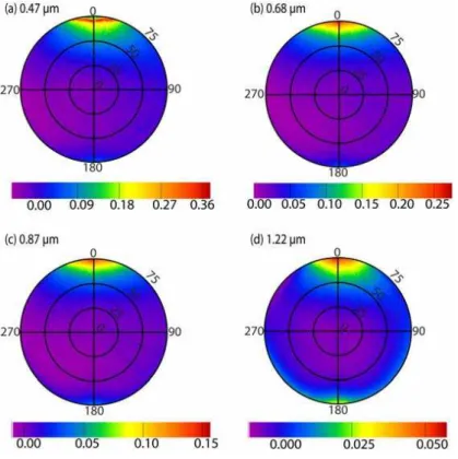
Figure 6 shows the error of atmospheric correction at wavelengths 0.47, 0.67, 0.87 5

and 1.22 µm when a Lambertian surface model is assumed. As is well known, the Lambertian assumption reduces the anisotropy of the BRF. It overestimates BRF at low view zenith angles, where BRF is lowest, and significantly underestimates it where the BRF is high, in the glint and hotspot regions. The error decreases with increasing wavelength. For example, the average reflectance overestimation at low θ is 0.02– 10

0.025, 0.01–0.015, 0.008–0.012, and 0.006–0.008 at 0.47, 0.67, 0.87, and 1.22 µm, respectively. The maximum error at θ=60◦ in the forward scattering direction at the same wavelengths is₋0.18,₋0.10,₋0.064 and₋0.026, respectively. In all the ARC-TAS snow experiments, the atmosphere was relatively clear (see Table 2). The error will be higher under hazy conditions, due to increased atmospheric scattering.

15

7 Analysis of AART model

The Analytical Approximate Radiative Transfer model (see Appendix A) predicts snow bidirectional reflectance as a function of snow grain size and level of absorbing impuri-ties, such as soot. The analytical form of this model makes it very convenient for snow grain size retrievals, and several approaches have recently been developed (Tedesco 20

and Kokhanovsky, 2007; Lyapustin et al., 2009; Kokhanovsky and Schreier, 2009). The AART model was tested against snow pit measurements (Kokhanovsky et al., 2005). Contrary to our results, the AART model was found to overestimate measured BRF in the glint region under specific conditions of measurements. Nevertheless, this work, and a broad-scale analysis of MODIS data over Greenland (Lyapustin et al., 2009), 25

(18)

ACPD

9, 21993–22040, 2009

ARCTAS

A. Lyapustin et al.

Title Page

Tables Figures

◭ ◮

Back Close

Full Screen / Esc

Interactive Discussion at angles close to the backscattering direction as well. These errors, discussed in the

introduction, are inherited from the plane-parallel radiative transfer solution (function

R0in Eq. (A3) of Appendix A).

In this section, we study the effect of macroscopic surface roughness on snow bidi-rectional reflectance. Roughness affects snow reflectance in two ways, via the variety 5

of slopes, which requires averaging the plane-parallel solution over a slope distribution function, and via shadows. In this work, we use a Gaussian slope distribution function with averaging procedure described in Appendix B. The model of snow shadows de-scribed in Appendix C may be considered as oversimplified, and yet it allowed us to achieve a relatively good match with BRF derived from the CAR measurements. 10

7.1 Averaging over slope distribution function

Figure 7a–f show the effect of averaging over a slope distribution function for several values of standard deviationσ=0, 0.2, 0.4. Figure 7a–c show results for a model us-ing spheroids (Dubovik et al., 2006) to compute the snow scatterus-ing function. The reflectance of a semi-infinite medium is computed with the SHARM code (Lyapustin, 15

2005) for zero absorption and an optical thickness of 20 000, which provides an asymp-totic reflectance limit. The results are shown for a grain size of 50 µm. Because there is no absorption, we did not find any noticeable difference in the radiative transfer solu-tion when the grain size varied from 20 to 200 µm. Figure 7a shows the deviasolu-tion of the plane-parallel solution (σ=0) from the experimental BRF computed asRmeas−Rmodel. It 20

overestimates the CAR BRF by 1.21 in the glint region maximum, and underestimates it by 0.31 in the backscattering direction. Averaging over slopes decreases the forward peak of the theoretical reflectance and increases its backscattering value, thereby re-ducing the differences with experimental data. Atσ=0.4, the difference in the forward and backscattering peaks is reduced by a factor of 3 (₋0.42) and 2 (0.166), respec-25

tively, atθ=76◦.

(19)

ACPD

9, 21993–22040, 2009

ARCTAS

A. Lyapustin et al.

Title Page

Tables Figures

◭ ◮

Back Close

Full Screen / Esc

Interactive Discussion (Mishchenko et al., 1999). In addition to errors in the rainbow angles, which are usually

not observed over snow, at least for visible wavelengths, the Mie model fits the CAR BRF poorly in the forward scattering region, where the error remains inhomogeneous and large over a wide range of azimuths and view zenith angles. The fractal model has an interesting pattern around the forward scattering peak, underestimating BRF at its 5

center and overestimating it at angles 30–60◦ offcenter. For the experiment geome-try (θ0=68.6◦), this suggests that the peak of the fractal phase function is too narrow and the phase function is underestimated at scattering angles below _∼50◦, while at the same time, it is overestimated at scattering angles ∼60–90◦. Comparing phase functions for the spheroid and random fractal models, Fig. 8 shows that this is indeed 10

the case. Except for the extremely narrow di_ffraction peak, the fractal phase function is significantly lower at angles below 28◦, and it is higher than the spheroidal model at angles above_∼39◦. Overall, the fractal model gives a much better fit in the backscat-ter region, where the error is a factor of _∼2 lower than that of the spheroid model. Given these considerations, we constructed a synthetic phase function from the 50 µm 15

spheroid and fractal models as follows:xSynth(γ)=xSPD(γ) at scattering anglesγ<37◦;

xSynth(γ)=(xSPD(γ)+xFract(γ))/2 at 37◦≤γ≤60◦;xSynth(γ)=xFract(γ) atγ≥90◦; and finally, in the range 60◦<γ<90◦, xSynth(γ) was obtained by linear interpolation between the

xSynth(60◦) and xSynth(90◦) values. For normalization, the resulting scattering function was reduced by a factor of 1.103. Figure 7f shows this result for the synthetic BRF 20

with slope averaging (σ=0.4). One can see the reduction in the total difference with the CAR BRF down to (₋0.1; 0.12) for the full range of θ_≤76◦, which is an improvement over all other cases. It is possible that specialized particle shapes modeling ice crys-tals (e.g., Xie et al., 2006; Jin et al., 2008) may provide an even better agreement with experimental data.

(20)

ACPD

9, 21993–22040, 2009

ARCTAS

A. Lyapustin et al.

Title Page

Tables Figures

◭ ◮

Back Close

Full Screen / Esc

7.2 Effect of shadows

In contrast to the slope averaging, shadows are not visible in the backscatter direction, where they don’t change the absolute value of reflectance. In our case, this represents the anglesθ≥θ0 atϕ=180◦. On the other hand, shadows act to increase the relative value of the backscattering peak by decreasing reflectance at other angles. Figure 7g–l 5

shows the effect of shadows on the BRF for two values of increased sastrugi density (D=0.04, 0.08). The images (g–i) are computed for the spheroid model atσ=0.4, and the images (j–l) show results for the synthetic model atσ=0.3. Figure 7i and l reproduce Fig. 7h and k at an expanded scale to show the fine details. Here, the black colors show values above the upper limit and below the lower limit of the color bar. One can see that 10

the best approximation of the CAR BRF for flight 2001b is obtained with the Synthetic model, providing accuracies within₋0.02 to+0.07 at θ_≤60◦. Finally, Fig. 7m shows the theoretical model fit for experiment 2005a, which had a different solar zenith angle (61.95◦). In this case, a good approximation, within±0.06 atθ≤60◦, was achieved with the Synthetic model and parametersσ=0.2,D=0.10, close to values for the previously 15

considered experiment 2001b.

7.3 Spectral analysis

If snow reflectance R0 is known for the nonabsorbing shortwave channel, then the AART model can predict the spectral dependence of snow BRF analytically (Eq. (A3), Appendix A):

20

ρ=R0(µ0,µ, ϕ) exp(−A(µ0,µ, ϕ) r

4πχ d

λ ). (7)

Assuming the functionR0 is computed with the synthetic BRF model and parameters (σ=0.3,D=0.08), we analyzed the accuracy of the AART model at 0.681, 0.871, 1.03, 1.22, 1.27, 1.654 and 2.204 µm wavelengths, for CAR flight 2001b. Based on the the-oretical derivation, the AART model is valid for

q 4πχ d

λ ≪1, limiting it to the visible-NIR

(21)

ACPD

9, 21993–22040, 2009

ARCTAS

A. Lyapustin et al.

Title Page

Tables Figures

◭ ◮

Back Close

Full Screen / Esc

Interactive Discussion spectral range of low absorption. So, our analysis at 1.654 and 2.204 µm wavelengths

for high snow absorption should be considered as formal only. The imaginary part of the refractive index of ice was taken from Warren and Brandt (2008).

Conducting this analysis requires knowledge of parameter d. The snow grain size (diameter) for this exercise was first evaluated from CAR BRF data using a method 5

developed for MODIS (Lyapustin et al., 2009), and based on the ratio of the NIR (λ1=1.22 µm) to red band (λ2=0.68 µm) reflectances. In this case, the AART model gives an analytical expression for the optical snow grain diameter:

d = 1 4πA2

ln

_ρ 1

ρ2

/

q

χ2/λ2− q

χ1/λ1 2

. (8)

Compared to the single-band algorithms for snow grain size retrievals (e.g. Nolin and 10

Dozier, 1993; Stamnes et al., 2007; Tedesco and Kokhanovsky, 2007), which depend directly on the functionR0and on its view-geometry-dependent errors, the band ratio algorithm to some extent suppresses these errors, reducing them to a second-order effect through the function A. We have done analysis with all of the previously de-scribed models (Sect. 7.1 and 7.2) and found that the synthetic model with (σ=0.3, 15

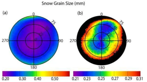
D=0.08) provides about the smallest dispersion of retrieved grain size as well. Figure 9 shows the grain size retrieval with this model for experiment 2001b. There is no reg-ular dependence of retrieved grain size at a relatively low view zenith angleθ<35–40◦. At higher view angles (_≥45–50◦), the retrieved d systematically grows withθ0 due to uncompensated BRF. Such dependence was observed from MODIS over Greenland 20

(Lyapustin et al., 2009). From the reduced-scale image of Fig. 9, the average grain size atθ<50◦can be assessed as_∼0.24_±0.03 mm.

Further, the valued=0.24 mm was used to study the spectral accuracy of the AART model. The results of this analysis are shown in Fig. 10. The three numbers above each image give the wavelength and parametersσandD. In the low absorption region, 25

(22)

ACPD

9, 21993–22040, 2009

ARCTAS

A. Lyapustin et al.

Title Page

Tables Figures

◭ ◮

Back Close

Full Screen / Esc

Interactive Discussion parametersσ=0.2 and D=0.10. At these wavelengths, the photon penetration depth

is only a few millimeters. Thus, increasing absorption essentially increases the weight of the small-scale surface roughness (several mm vs. several tens of cm) in averaging over the slope distribution function.

The maximal size of the high slope facets in the area of field measurements was only 5

5–10 cm (see also Fig. 1). With the average photon penetration depth of 30 cm in the visible spectrum, the assumption of independently scattering facets may not be entirely valid. Thus, the obtained valueσ=0.3 may be considered as a model result providing a good fit to the measurements. On the other hand, conditions for averaging are met in the near infrared, and valueσ_∼0.2 may be better related to a surface roughness. 10

At the high absorption wavelengths (λ=1.65, 2.2 µm), the plane-parallel solution (σ=0) with the synthetic model provides the best fit to the CAR BRF. In all wavelengths, the accuracy of the theoretical solution is close to the CAR BRF to within about_±0.05 over the full range of MODIS view anglesθ_≤55₋60◦, including the forward scattering and backscattering directions.

15

8 Conclusions

The spring 2008 ARCTAS experiment was one of the major intensive field campaigns of the International Polar Year aimed at detailed characterization of atmospheric and surface properties of the Arctic region. In this work, we focused on processing and analysis of CAR-AATS-AERONET data from a rather unique snow bidirectional re-20

flectance P-3B airborne experiment. The goals of this study included obtaining snow bidirectional reflectance at high 1◦ angular resolution from CAR measurements and using these data for an accuracy analysis of analytical RTLS, MRPV and AART BRF models over snow. Another major goal was developing a model of macroscopic surface roughness that would adjust the plane-parallel radiative transfer solution to experimen-25

tal snow BRF. The main results of this work may be summarized as follows:

(23)

ACPD

9, 21993–22040, 2009

ARCTAS

A. Lyapustin et al.

Title Page

Tables Figures

◭ ◮

Back Close

Full Screen / Esc

Interactive Discussion evaluated. The BRF and albedo are produced for 3 flight segments on 7 April and

a flight segment on 15 April. The BRF and albedo are consistent on these two dates, and between different flight altitudes on the first date. Except for the red band, the derived CAR albedo is consistent with ground albedo measurements. The files containing the CAR measurements and derived spectral snow BRF can 5

be found at http://car.gsfc.nasa.gov/data/index.php?mis id=8&n=ARCTAS&l=h. 2. The surface albedo derived from CAR data generally concurred with ground

mea-surements.

3. The obtained snow BRF is significantly anisotropic, even in the cross-plane. The derived BRF pattern from CAR measurements is similar to the measurements of 10

Hudson et al. (2006) made over Antarctica from a 32 m tower. The use of Lam-bertian assumption for atmospheric correction may lead to large errors, especially in the shortwave channels.

4. Except for forward scattering (glint) region of angles ϕ<40◦, the best fit MRPV and RTLS models provide a good fit to CAR BRF measurements to within±0.05. 15

Overall, the RTLS model gives a better fit in the forward scattering angles, whereas the MRPV model suits snow reflectance better in the backscattering directions.

5. In agreement with the previous studies, the plane-parallel radiative transfer solu-tion was found to have large errors in the broad range of angles near the forward 20

scattering and backscattering directions. Regardless of the shape of snow grains, the plane-parallel model significantly overestimates snow BRF in the broad glint region and underestimates it in the backscattering domain. Fitting CAR BRF data shows that the randomly oriented fractal model and the model of spheroids work much better than the Mie solution, and have complementary abilities in fitting the 25

(24)

for-ACPD

9, 21993–22040, 2009

ARCTAS

A. Lyapustin et al.

Title Page

Tables Figures

◭ ◮

Back Close

Full Screen / Esc

Interactive Discussion ward scattering angles, and is a fractal model in the backscattering range. The

radiative transfer solution with synthetic phase function was found to fit measured BRF in the full range of angles better than any individual model.

6. For the first time, we introduced averaging of the plane-parallel radiative transfer solution over the slope distribution function that accounts for a natural snow sur-5

face roughness. Due to large snow grain sizes (compared to the wavelength), the scattering function of snow is rather flat in the backscattering domain and cannot provide the increase of reflectance at backscattering angles required to match observations. In these conditions, introducing rather steep slopes is perhaps the only way to increase snow reflectance at backscattering angles (see also Hud-10

son and Warren, 2007). We found that averaging over slope distribution strongly reduces the difference between theoretical model and observations and allows us to model both the forward and backscattering regions with good accuracy at relatively high zenith angles.

7. Adding shadows, even via a very simple model, was found to further reduce the 15

difference between the CAR data and the model.

8. A spectral-angular analysis showed that the AART model with the fitted surface roughness parameters σ and D provides an accuracy of about ±0.05 with the possible bias of _±0.03 in the spectral range 0.4–2.2 µm at θ_≤55–60◦, including forward- and backscattering domains.

20

(25)

ACPD

9, 21993–22040, 2009

ARCTAS

A. Lyapustin et al.

Title Page

Tables Figures

◭ ◮

Back Close

Full Screen / Esc

Appendix A

Analytical BRF models

A Ross–Thick Li-Sparse (RTLS) BRF model (Lucht et al., 2000):

ρ=kL+kGf_G(µ₀,µ, ϕ)+kVf_V(µ₀,µ, ϕ). (A1) 5

Here, subscripts refer to isotropic (L), volumetric (V) and geometric optics (G) com-ponents. It uses predefined geometric functions (kernels) fG,fV to describe different

angular shapes. The kernels are independent of the land conditions. The BRF of a pixel is characterized by a combination of three kernel weights, K={kL, kG, kV_}T. The RTLS model is used in the operational MODIS BRF/albedo algorithm (Schaaf et 10

al., 2002).

A Modified Rahman-Pinty-Verstraete (MRPV) model:

ρ=ρ0M(k)F(b)H(ρ0), (A2)

M(k)=[µµ₀(µ+µ₀)]k−1, F(b)=exp(₋bcosγ), H(ρ0)=

1+1−ρ0 1+G

,

where γ is angle of scattering, cosγ=−µ₀µ+ q

1₋µ2₀p1₋µ2_cos(_ϕ₋_ϕ

0), and 15

G= q

tg2_θ₀₊_tg2_θ₊₂_tgθ

0tgθcos(ϕ−ϕ0). The MRPV model yields a nearly linear ex-pression for the model parameters after logarithmic transformation (Martonchik et al., 1998).

An Analytical Approximate Radiative Transfer model (AART) (Kokhanovsky and Zege, 2004):

20

ρ=R0(µ0,µ, ϕ) exp(−A(µ0,µ, ϕ) p

γd). (A3)

Here,γ=4πχ /λ, χ is imaginary part of refractive index of ice, λis a wavelength, and

(26)

ACPD

9, 21993–22040, 2009

ARCTAS

A. Lyapustin et al.

Title Page

Tables Figures

◭ ◮

Back Close

Full Screen / Esc

Interactive Discussion the average surface area of grains. R0is an RTE solution for semi-infinite media (the

Milne’s problem) with zero absorption. For simplicity, we assume that R0 does not depend on snow grain size because λ_≪d (50 µm for fresh snow to 200 µm in pre-melting conditions (Wiscombe and Warren, 1980) to 1–1.5 mm during snowmelt). The functionArelates to the photon’s escape probability from the media. For the fractal ice 5

particles, it can be approximated as follows:

A(µ0,µ, ϕ)∼=0.66(1+2µ0)(1+2µ)/R0(µ0,µ, ϕ). (A4)

Appendix B

Integration of plane-parallel solution with a slope distribution function

10

Even over a flat ice, the snow surface exhibits height/slope variations due to snow re-distribution by wind and gravity. The reflectance of an individual facet can be modeled with the plane-parallel solution if the depth of snow behind the facet is comparable with the photon penetration depth (defined as a depth at which radiative flux is reduced by a factor of e). In the visible range (0.4–0.8 µm), the snowpack attains properties of 15

a semi-infinite layer at depths varying from about 20 cm for a new (fine grained) snow to about 50 cm for an old snow (e.g., Wiscombe and Warren, 1980; Zhou et al., 2003). Snow becomes moderately absorptive in the near infrared (1.24 µm) where photon depth penetration is in the range of_∼0.55 cm for 100 µm grains to_∼1.3 cm for 500 µm grains (Li et al. 2001; Lyapustin et al., 2009). In the wavelength region of 1.5–2.2 µm 20

(27)

ACPD

9, 21993–22040, 2009

ARCTAS

A. Lyapustin et al.

Title Page Abstract Introduction Conclusions References Tables Figures ◭ ◮ ◭ ◮ Back Close

Full Screen / Esc

Interactive Discussion visible (not in the shadow), the total reflectance can be written as follows:

Rnew(µ0,µ, ϕ)= 1 µ0N

2π Z 0 1 Z 0

µ01R(µ01,µ1, ϕ1)P(µn, ϕn)dµnd ϕn. (B1)

For the lack of better assumption, we will use an azimuthally independent Gaussian probability density function of slope distributions (Nakajima and Tanaka, 1983)

P(µ_n)₌ 1

πσ2_µ3

n

exp ₋1−µ 2

n

σ2_µ2

n

!

, (B2)

5

where µ_n is cosine of zenith angle of the vector of normal. This model may not be valid in the world regions as Antarctica with predominant wind direction that creates sastrugi oriented perpendicular to the blowing wind (Hudson et al., 2006).

Numerically, Eq. (B1) is interpreted as follows. Let us define a reference right-handed coordinate system (x, y, z). Let the solar plane coincide withx-axes, ϕ0=180◦. The 10

vectors of incidence and reflection are defined by the directional cosines (or projections of a unit vector on each axis): for example, incidence vector isI=(₋q1₋µ2₀,0,−µ₀) and view vector isV=(₋p1₋µ2_cos_ϕ,p₁₋_µ2_sin_ϕ,_{µ). The minus sign at the} _x_-projection accounts for the fact that the relative azimuth is defined with respect to the solar az-imuth (ϕ=ϕ−ϕ0).

15

Next, for every orientation of a facet we define a new coordinate system (x_n, y_n, z_n) rotated in azimuthϕ_nabout axiszand then rotated in angleθ_n(µ_n=cosθ_n) about axis

y. The new coordinates of incidence and view vectors are related to the initial values by a rotation transformation, e.g.V1=T_θ_nT_ϕ_nV, where rotation matrices are

T_ϕ = 



cosϕ sinϕ 0

−sinϕcosϕ0

0 0 1



 , T_θ = 



cosθ0₋sinθ

0 1 0

sinθ 0 cosθ



(28)

ACPD

9, 21993–22040, 2009

ARCTAS

A. Lyapustin et al.

Title Page

Tables Figures

◭ ◮

Back Close

Full Screen / Esc

Interactive Discussion To reduce computations and avoid numerical uncertainties caused by a definition of

inverse cosine and inverse tangent, only new zenith angles (µ₀₁,µ₁) are computed using rotation matrices while the new relative azimuth (ϕ1) is calculated based on invariance of the scattering angle with respect to the rotation of the coordinate system. Because zenith view and sun angles cannot be larger than 90◦ in the rotated co-5

ordinate system (for plane-parallel model to hold), not every pair of zenith and az-imuthal quadrature angles can be realized in Eq. (A1). In other words, for all geome-tries except nadir view and sun in zenith, only part of the upper hemisphere can be both illuminated and visible. This restriction is implemented through a joint constraint µ01≤0, µ1≥0. For this reason, the integrated solution needs a normalization coeffi -10

cient, N= 2π

R

0 1 R

0

P(µn, ϕn)dµnd ϕn computed with the same constraint, which effectively

shows the part of the hemisphere that is simultaneously illuminated and visible to the observer. The integration of Eq. (B1) is performed numerically using Gaussian quadra-ture and a look-up table of functionR pre-computed with small step for the full range of azimuths and a range of zenith angles µ₀,µ ₌ 1–0.12. The specific reflectance at 15

quadrature points is obtained by 3-D interpolation in angles.

Appendix C

Shadow factor

The macroscopic surface roughness creates shadows that change bidirectional re-20

flectance of snow. Even though shadowed areas are illuminated by the di_ffuse sky light, for simplicity we assume that shadows don’t contribute into reflected signal. Here, we also ignore 3-D effects of horizontal diffusion of photons inside snow from illuminated into the shadowed area. This e_ffect may be important in the visible part of spectrum, but it becomes negligible in the near infrared because of increased snow absorption. 25

(29)

ACPD

9, 21993–22040, 2009

ARCTAS

A. Lyapustin et al.

Title Page

Tables Figures

◭ ◮

Back Close

Full Screen / Esc

Interactive Discussion area in the footprint:FSh=(1₋SSh/S).

To compute shadow area, let us use a simple model of surface roughness as hemi-spheric protrusions of radius (height)requidistantly spaced at a distanceR. To simplify our model further, we assume that all of the shadow comes from illuminated half of the hemisphere (as if the sun were at horizon,θ0=90◦). In this case, the area of a shadow 5

viewed at nadir isSSh=πr22tgθ0. When the shadow is not subtended by the protru-sion, the shadow area does not depend on the relative azimuth. This is approximately true for the forward scattering directions (|ϕ|≤90◦). In the backscattering directions, the shadow area will be reduced asSSh_∼πr₂2(tgθ0+tgθcosϕ), wheretgθ0+tgθcosϕ_≥0. This formula is exact in the principal plane in the backscattering direction (ϕ=180◦) and 10

in the cross-plane. Assuming that this expression is approximately valid for the other backscattering angles, we can write the final formula for the shadow factor:

FSh=1₋πD 2

2 H(θ0, θ, ϕ), where H(θ0, θ, ϕ)=

tgθ0,|ϕ| ≤90◦

tgθ0+tgθcosϕ,|ϕ|>90◦

,(C1)

andD=r/R is density of protrusions. Although oversimplified, this shadow model pre-dicts an overall correct angular dependence added by snow shadows. It has an ad-15

vantage of dependence on a single parameter (density) that makes it rather robust for the remote sensing of snow given all sources of uncertainties and variability in model-ing roughness of natural snow. Because of simplifications, such as neglectmodel-ing diffuse irradiance of the shadowed areas, the best-fit parameter D matching experimentally measured BRF may differ from the real roughness density characterizing field condi-20

tions.

The total snow reflectance accounting for slope distribution and shadows becomes:

ρ(µ₀,µ, ϕ)₌Rnew(µ₀,µ, ϕ)FSh. (C2) Acknowledgements. The research of A. Lyapustin and Y. Wang was funded by the NASA Ter-restrial Ecology Program (Dr. Wickland). Research by C. K. Gatebe and R. Poudyal was

spon-25