560 MULTIPLE SOLUTIONS FOR AN EQUATION OF KIRCHHOFF TYPE

(1)

doi: 10.5540/tema.2018.019.03.0559

Multiple Solutions for an Equation of Kirchhoff Type:

Theoretical and Numerical Aspects

A.L.M. MARTINEZ1, E.V. CASTELANI2, G.M. BRESSAN1and E.W. STIEGELMEIER1

Received on March 15, 2018 / Accepted on June 25, 2018

ABSTRACT. A nonlinear boundary value problem related to an equation of Kirchhoff type is considered. The existence of multiple positive solutions is proved through Avery-Peterson Fixed Point Theorem. A numerical method based on Levenberg-Marquadt algorithm combined with a heuristic process is present in order to align numerical and theoretical aspects.

Keywords: Multiple solution, Kirchhoff Equation, numerical solutions.

1 INTRODUCTION

In this paper we present a study on second order equation Kirchhoff problem, given by

(

M(ku′_k2₂)u′′₊_q(t₎_f_(t_,_u_,_u′_{) =}₀

u(0) =0,u(1) =0 (1.1)

whereM:R→R,f :[0,1]×R×R→Randq:R+→Rare continuous maps.

Variations of (1.1) can be related to stationary state of Kirchhoff equation [8]. For example, as elucidated in [11] considering argument reflection and later in [1] with more general boundary conditions a stationary state of the Kirchhoff equation of kind of:

utt−

c0+c1

Z L

0 | ux|2dx

uxx=0, (1.2)

can be associated with their respectives equations. This kind of equation commonly appear in the context of free vibrations in elastic strings, consequently, they form a relevant object of study.

Many authors have studied problems related to (1.2). For a wide spectrum of study, we recom-mend [2], [3], [6], [10] and more recently [5]. Concerning the problem (1.1) we can observe

*Corresponding author: Andr´e Lu´ıs Machado Martinez – E-mail: [email protected]

1Departamento Acadêmico de Matemática, Universidade Tecnológica Federal do Paraná, Cornélio Procópio, PR, Brasil. E-mail: [email protected], [email protected], [email protected]

(2)

by [12] that studies with theoretical aspects were developed using Banach’s Fixed Point Theo-rem or Leray-Schauder Alternative combined with Krasnoselskii’s TheoTheo-rem. Consequently, it is natural to ask about existence results by using Avery-Peterson Theorem [4]. In this sense, this work complement previous results of existence with the cited theorem, and this study is present in Section 2.

Numerical studies related to second order equations, normally, are presented as illustration of the existence Banach’s Fixed Point Theorem applied to equation but no strategy is given to ilus-traste more general results (like the existence results provided by Avery-Peterson Theorem). The common sense suggests that optimization methods combined with heuristic processes can provide good results to find multiple numerical solutions. As consequence, a method based on Levenberg-Maquardt [13, 9] is shown in Section 3 and comparisons with other methods using classical strategies are established. Still, in Section 3, a simple but effective heuristic process is introduced in order to find multiple numerical solutions. Final remarks are given in Section 4.

2 MULTIPLE SOLUTIONS

LetC1[0,1] be the Banach space of the continuously differentiable functions in[0,1]. Let us considerE={u_∈C1[0,1];u(0) =u(1) =0}with the norm

ku_kE=ku′k∞.

We begin this section by observing that the solutions of (1.1) can be written as:

u(t) =

Z 1

0

G(t,s)q(s)f(s,u(s),u′(s)) M(ku′_k2

2)

ds, (2.1)

whereGis the Green’s function

G(t,s) =

(

s(1−t), s_≤t t(1−s), t_≤s .

Considering the result that we will show, we must note some properties of the functionG. In fact, we have that

∂tG(t,s) =

(

−s, s_≤t 1−s, t_≤s ,

thenGsatisfies:

G(t,s) =|G(t,s)| ≤ |∂tG(t,s)|. (2.2)

Letmbe a constant in[0,1/2]. Thus, we can obtain the inequalities

G(t,s)≥mG(s,s),∀x_∈[m,1−m] (2.3)

and

(3)

Thus, concerning the representation given in (2.1) we define the operatorT :E_→Eas:

T(u) =

Z 1

0 G(t,s)q(s)

f(s,u(s),u′(s)) M(ku′_k2₂) ds,

whereMandf are assumed to be continuous functions and there is a constantM0>0 such that M(y)≥M0for allyin the domain ofM.

We claim thatT is continuous and completely continuous. Continuity follows immediately from the Lebesgue dominated convergence theorem and the fact that

|T(u)(t)−T(un)(t)| ≤ Z 1

0 G(t,s)q(s)

f(s,u(s),u′(s)) M(ku′_k2

2)

− f(s,un(s),u′n(s))

M(ku′_n_k2 2) ds, ≤ Z 1 0

G(s,s)q(s)

f(s,u(s),u′(s)) M(ku′_k2

2)

− f(s,un(s),u′n(s)) M(ku′

nk22)

ds, ≤ Z 1

0 s(1−s)q(s)

f(s,u(s),u′(s)) M(ku′_k2₂) −

f(s,un(s),u′n(s)) M(ku′_n_k2₂)

ds,

withun,u∈E. To show complete continuity we will use the Arzela-Ascoli’s theorem. LetΩ⊆E be bounded, in other words, there existsΛ0>0 withkuk ≤Λ0for eachu∈Ω. Now ifu∈Ωwe have

|(Tu)′(t)| ≤

Z 1

0 |

G′(t,s)|H_Λ₀(s)ds

where H_Λ₀ is determined by the bounded set and functionsq, f and M. It is easy to check that H_Λ₀(s)∈L1[0,1]. Then imply that T_Ω is a bounded equicontinuous family on [0,1]. Consequently the Arzela-Ascoli theorem impliesT :E_→Eis completely continuous.

Consider the following hypotheses:

(A1) There are positive constantsd, A,Bsuch that:

• q(t)f(t,u,v)≥0, ∀(t,u,v)∈[0,1]×[−d

2, d

2]×[−d,d];

• ∀(t,u,v)∈[0,1]×[−d

2, d

2]×[−d,d], then|f(t,u,v)| ≤ dA

r1 ,where

r1=max t∈[0,1]

Z 1

0 |∂tG(t,s)q(s)| ds

;

• A_≤M(ku′_k2₂)≤ B,∀ ku_kE≤d;

Next, we define a conePby

P={u_∈C1[0,1];u_≥0,u(0) =u(1) =0}.

Remark 1.Denoting

F(t) =

Z 1

0

(4)

we can extract some properties related to F. Since

F′′(t) =−q(t)f(t,u(t),u′(t)) M(ku′_k2

2)

≤0,

from(A1), we find that F is concave, and since F(0) =F(1) =0, we can conclude that

min t∈[1

4,34]

Z 1

0 G(t,s)q(s)

f(s,u(s),u′(s)) M(ku′_k2

2)

ds=min

Z 1

0 G( 1 4,s)q(s)

f(s,u(s),u′(s)) M(ku′_k2

2) ds,

Z 1

0 G(3

4,s)q(s)

f(s,u(s),u′(s)) M(ku′_k2

2) ds

For the purpose of this work we need to introduce the main tools.

Avery-Peterson theorem.

Now, we need to consider the convex sets

P(γ,d) ={x_∈P_|γ(x)<d_}

P(γ,α,b,d) ={x_∈P_|b_≤α(x)andγ(x)<d_}

P(γ,θ,α,b,c,d) ={x_∈P_|b_≤α(x),θ(x)≤candγ(x)<d_}

and the closed set

R(γ,ψ,a,d) ={x_∈P_|a_≤ψ(x)andγ(x)<d_}.

Theorem 2.Let P be a cone in a real Banach space X . Let γ and θ nonnegative continuous convex functionals on P,α be a nonnegative continuous concave functional on P, andψ be a nonnegative continuous functional on P satisfyingψ(λx)≤λ ψ(x)for0≤λ≤1, such that for some positive numbersµand d,

α(x)≤ψ(x)and_kx_{k ≤}µγ(x),

for all x_∈P(γ,d). Suppose

T :P(γ,d)→P(γ,d)

is completely continuous and there exist positive numbers a, b, c with a<b, such that

{u_∈P(γ,θ,α,b,c,d)|α(u)>b_{} 6}=/0and

u_∈P(γ,θ,α,b,c,d)⇒α(Tu)>b (2.5)

α(Tu)>b for u_∈P(γ,α,b,d)withθ(Tu)>c, (2.6)

06∈R(γ,ψ,a,d)andψ(Tu)<a for (2.7)

(5)

Then T has at least three distinct fixed points in P(γ,d).

In our main result (given by Theorem 2) we will show that the Problem 1.1 has at least three positive solutions.

Theorem 3.Suppose that the hypothesis(A1)is satisfied. Suppose, in addition, that there exist a,0<a<d such that f satisfies the following conditions:

(A2) |f(t,u,v)|<Aa

r2

,_∀(t,u,v)∈[0,1]×[0,a]×[−d,d],

where r2=max t∈[0,1]

Z 1

0 G(t,s)|q(s)| dt

.

(A3) |f(t,u,v)|>2aB

r3

,_∀(t,u,v)∈[0,1]×[2a,8√2a]×[−d,d],

where r3=min

Z 1

0 G( 1

4,s)|q(s)|ds,

Z 1

0 G( 3

4,s)|q(s)|ds

.

Then, Problem (1.1) has at least three positive solutions.

Proof. We will apply Avery-Peterson theorem (as stated in [4]). Let us considerT andP as defined before. Furthermore, we need define the following functionals

γ(u) = ku_kE,

ψ(u) = max t∈[0,1]|u(t)|,

θ(u) =

"

Z 3

4

1 4

[u(t)]2_dt

#1₂

,

α(u) = min

t∈[1 4,34]

|u(t)|.

Therefore, we need to verify that

T:P(γ,d)→P(γ,d)

is completely continuous and there exist positive numbersbandcwitha<b, such that

{u_∈P(γ,θ,α,b,c,d)|α(u)>b_{} 6}=/0 and

u_∈P(γ,θ,α,b,c,d)⇒α(Tu)>b (2.8)

α(Tu)>bforu_∈P(γ,α,b,d)withθ(Tu)>c, (2.9)

06∈R(γ,ψ,a,d)andψ(Tu)<afor (2.10)

(6)

Using(A1)we haveTu_≥0 ifγ(u) =ku_kE≤d, and obtain:

kTu_kE = k(Tu)′k∞

≤ dA_r

1 max t∈[0,1]

Z 1

0

|∂xG(t,s)q(s)| M(ku′_k2

2) ds

≤ d.

ThereforeT appliesP(γ,d)inP(γ,d).

Now, we consider

b=2a

and

c=8√2a.

Clearly, we have{u_∈P(γ,θ,α,b,c,d)|α(u)>b_{} 6}=/0. Let us demonstrate (2.8). Using (A3) we obtain

α(Tu) = min

t∈[1 4,34]

(Tu)(t)

= min

t∈[1 4,34]

Z 1

0

2) ds

= min

x∈[1 4,34]

Z 1

0

G(t,s)|q(s)||f(s,u(s),u′(s))|

M(ku′_k2 2) ds = min Z 1 0 G(1

4,s)|q(s)|

|f(s,u(s),u′(s))|

M(ku′_k2 2)

ds, Z 1

0 G(3

4,s)|q(s)|

|f(s,u(s),u′(s))|

M(ku′_k2 2) ds > 2aB r3 min Z 1 0 G( 1 4,s)

|q(s)|

M(ku′_k2 2)

ds,

Z 1

0 G( 3 4,s)

|q(s)|

M(ku′_k2 2) ds > 2a r3 min Z 1 0 G( 1

4,s)|q(s)|ds,

Z 1

0 G( 3

4,s)|q(s)|ds

≥ 2a=b.

(7)

α(Tu) = min t∈[1

4,34] Z 1

0

2) ds ≥ 1 4 Z 1 0

2) ds

≥ 1

4tmax∈[0,1]

Z 1

0 G(t,s)q(s)

f(s,u(s),u′(s)) M(ku′_k2

2) ds

≥ 1

4√2θ

Z 1

0 G(t,s)q(s)

f(s,u(s),u′(s)) M(ku′_k2₂) ds

≥ 1

4√2θ(Tu)

> 1

4√2c=b.

Now, let us show (2.10). Thus, letu_∈R(γ,ψ,a,d)withψ(u) =a. From(A1)−(A2)we have,

ψ(Tu) = max

t∈[0,1]|Tu(t)|

≤ max t∈[0,1]

Z 1

0 G(t,s)q(s)

f(s,u(s),u′(s)) M(ku′_k2

2) ds

≤ max t∈[0,1]

Z 1

0

G(t,s)|q(s)||f(s,u(s),u′(s))|

M(ku′_k2 2)

ds

≤ Aa_r

2 max x_∈[0,1]

Z 1

0 G(t,s)

|q(s)|

M(ku′_k2₂)ds

≤ _ra

2 max x∈[0,1]

Z 1

0 G(t,s)|q(s)| ds

≤ a.

Applying Avery-Peterson theorem we obtain the result.

Example 2.1.This example shows a problem that has at least three positive solutions, according to Theorem 3. Suppose that

q(t) =1,

f(t,u,v) =

(

t+u3+ (v 55)

2_, ₀_≤_u_≤₃ t+24+u+ (₅₅v)2_, ₃_≤_u and

M(y) =0.7+0.4 sin2(y).

(8)

(A1)for(t,u,v)∈[0,1]×[0,55]×[−55,55]

r1= max x∈[0,1]

Z 1

0 |

∂tG(t,s)|ds= 1 2

0_≤f(t,u,v)≤1+24+55+1=76<77=55×0.7 0.5 =

dA r1

A_≤M(||u′_||2₂)≤B.

(A2)for(t,u,v)∈[0,1]×[0,1.5]×[−55,55]

f(t,u,v)≤1+ (1.5)3+1=5.375<8.4=λ1a r2

where

r2=max t_∈[0,1]

Z 1

0 |G(t,s)| ds=1

8.

(A3)for(t,u,v)∈[0,1]×[3,12√2]×[−55,55]

f(t,u,v)≥27>26.4=2×1.5×1.1

1/8 =

2aB r3

where r3=min

Z 1

0 G( 1 4,t)dt,

Z 1

0 G( 3 4,t)dt

=1

8.

Thus, from Theorem 3, the problem has at least three positive solutions.

3 NUMERICAL SOLUTIONS

In most studies, numerical solutions are obtained by fixed point methods, according to [12]. More specifically, an iterative sequence based on operator given by equation (2.1) define the method. The basic idea of the proposed method is to use the Levenberg-Maquardt algorithm [13]. This type of algorithm arises frequently in the context of optimization related to the data adjustment problem [7]. The Levenberg-Marquardt algorithm can be easily used for the solution of non-linear systems. Algorithm 1 briefly describes the ideas to solve the Problem (1.1).

(9)

Algorithm 1:

1. Define an uniformly spaced mesh{tj}, j=1, . . . ,n.

2. Choose initial approximationu0_j=u0(tj).

3. Discretize the Problem (1) by finite difference. Forj=2, . . . ,n₋1

• u′′k(tj) =

uk(tj+1)−2∗uk(tj)+uk(tj−1)

h2 ;

• u′k(tj) =

uk(tj+1)−uk(tj−1)

2∗h

approachingku′_k2₂by using trapezoidal rule. Thus we have the following linear system

r(uk) =0,

where

r(uk_{) =}

M(ku′_k2

2)u′′k(tj) +q(tj)f(tj,uk(tj),u′k(tj)) =0;j=2, . . . ,n−1.

4. Fork=1,2,3, . . .(Levenberg-Maquardt)

(a) Computerk= (r1,r2, . . . ,rn)T andAk= (ai j)n×n;

ri=ri(uk), ai j=∇ri(uk)

(b) Find∆ksuch that:

(ATkAk)∆k=−ATkrk.

(c) Determinesαksuch that the Armijo’s condition is satisfied.

(d) Compute

uk+1=uk+αk∆k.

5. Convergence test.

3.1 An heuristic procedure for initial approximations

We know the solutions that we are looking for must be concave or convex and will satisfy the conditionu(0) =u(1) =0. Thus, approaches by parabolas are reasonable ways of approaching the solution. In this sense, the heuristic procedure proposed in this paper consists in generating parables about initial points as follows:

(10)

wherenr is a random number in[− d 2,

d

2]. For practical purposes, the proposed procedure is defined by Algorithm 2.

Algorithm 2:

1. Choose a vectornr∈[−d₂,d₂]p.

2. Fork=1, ...,Ndo:

(a) Computeu0_k_,_i=u0_k(xi) =nr kxi(1−xi),i=1, ...,n (b) Run Algorithm 1 with initial approximationu0_k.

Naturally, this procedure returns multiple answers. So we need to establish a way to compare solutions in order to distinguish them. Note that the magnitude of the solutions may be different. In this sense, we say that the numerical solutionsu∗andu∗∗areequivalentif

ku∗₋u∗∗_{k ≤}max{10−8,10−6min{ku∗_k,ku∗∗_k}}. (3.1)

is satisfied.

Additional tests are run by using an algorithm based on the Banach Fixed Point Theorem. Con-sidering some hypothesis about the functions f andM, we can demonstrate, using the Banach Fixed Point Theorem (details in [12]), the local convergence of algorithms that use the iterative sequence

uk+1=T(uk₎_.

This procedure is described by Algorithm 3, which is a version of the algorithm proposed in [12].

Algorithm 3:

1. Define a uniformly spaced mesh{xj}em[0,1].

2. Choose initial approximationu0

j=u0(xj).

3. Fork=1,2,3, . . .

(a) Computeu′_jkby central-differences.

(b) Computeuk_j+1using

uk+1=T(uk)

where the integrals are computed using trapezoidal rule.

(11)

For practical purposes, the procedure is formalized by Algorithm 4, which is equivalent to Algorithm 2 and it calculates possible multiple solutions.

Algorithm 4:

1. Choose a vectornr∈[−d2, d 2]p. 2. Fork=1, ...,Ndo:

(a) Computeu0_k_,_i=u0_k(xi) =nr kxi(1−xi),i=1, ...,n (b) Run Algorithm 3 with initial approximationu0_k.

3.2 Examples

The examples below show how the Algorithm 2 can be promissor in order to find multiple solu-tions. We run Algorithm 2 and 4 withN=10. For Algorithm 3, we consider as stopping criteria:

kuk+1₋uk_k<10−4and for Algorithm 1 we considerkuk+1₋uk_k<10−6.

Example 3.1. Consider Problem (1.1) defined by

f(t,u,u′) =u,

and

M(y) = 1

π4y+ 1 2π2

The solutions areu(x) =sin(πt)andu(x) =0. In this example we considerd=10 andn=20 points for the spaced mesh. The numerical results are compared with the exact solution.

Running Algorithm 2, the procedure converged to the solution in 9 out of 10 times in which the Algorithm 1 was called. After 7 iterations of Algorithm 1, six initializations converged to the solution u and the obtained accuracy is max|u7₋_u_|₌₀_._{006189. After 4 iterations of} Algorithm 1, three initializations converged to the solution u and the obtained accuracy is max|u4₋u_|=1.092×10−13. The divergence means that the maximum number of iterations, i=50, was extrapolated. At the point where the execution stopped, the solution was near ofu.

On the other hand, running Algorithm 4, the procedure converged to the solution u (the less norm) in 8 out of 10 times in which the Algorithm 3 was called and reached the required accu-racy (kuk+1₋uk_k<10−4) afterkiterations, with 11≤k_≤14.The two divergences mean that Algorithm 3 stopped running since the functionM became null and then there was a divide by zero. For accuracy or order<10−4, the algorithm diverges in most of times, due to divide by zero.

Example 3.2. Consider the Problem (1.1) defined by

(12)

and

M(y) =0.1+9

√

2(y2₎1₄ 10π

The solutions areu(x) =sin(πt),u(x) =−sin(πt)andu(x) =0. In this example, we consider d=10 andn=20 points for the spaced mesh. The numerical results are compared with the exacts solutions.

Running Algorithm 2, the procedure converged to the solution in 10 out of 10 times in which the Algorithm 1 was called. After 5 iterations of Algorithm 1, five initializations converged to the solutionu and the obtained accuracy is max|u5₋u_|=0.00532072. After 5 iterations of Algorithm 1, three initializations converged to the solutionu and the obtained accuracy is max|u5₋u_|=0.00574833. After 12 iterations of Algorithm 1, two initializations converged to the solutionuand the obtained accuracy is max|u12₋u_|=0.000063816.

On the other hand, running Algorithm 4, the procedure converged to the solution null (the less norm) in 10 out of 10 times in which the Algorithm 3 was called and reached the required accuracy (kuk+1₋uk_k<10−4) afterkiterations, with 5≤k_≤7.

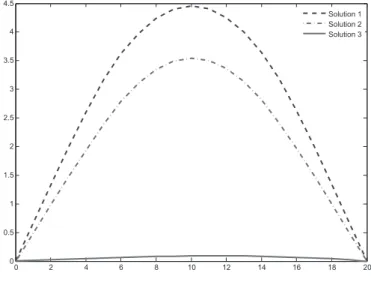
We have conducted an additional test, which run Algorithm 2 using the functions defined in Example 1. In this example, we definedn=20 and d=55. Using the criterion established in (3.1), we obtain that the 3 solutions are different. These results illustrate the result of existence given by Theorem 3. Figure 1 shows a graphical representation of these solutions.

0 2 4 6 8 10 12 14 16 18 20

0 0.5 1 1.5 2 2.5 3 3.5 4 4.5

Solution 1 Solution 2 Solution 3

(13)

Running Algorithm 4, the procedure converged to the solution of less norm in 9 out of 10 times in which the Algorithm 3 was called (according to the criteria described in 3.1) and reached the required accuracy (kuk+1₋_uk_k_<₁₀−4_{) after 5 iterations.}

As a conclusion, Algorithm 4 have found only the solution of less norm in all the run examples. On the other hand, Algorithm 2 have found, to the same run examples, all the possible solutions. Therefore, Algorithm 2 is more robust and suitable to determine multiple solutions.

4 FINAL REMARKS

Considering the numerical aspects of this work, we present a new algorithm (Algorithm 1) and a new heuristic that allows obtain multiple solutions. The method has robustness to solve second order equation Kirchhoff problem. Of course, the cost of this robustness is a slightly higher cost of computer processing, especially when we compare the method presented in last section with fixed-point methods (using the operator given by (7)).

Fortunately, the level of processing is not absurd even considering finer meshes. Furthermore, the method can be adapted for parallel programming and consequently, new features can be exploited in the computational field.

RESUMO. Um problema de valor de fronteira associado é uma equação do tipo Kirchhoff é considerado. Resultados de existência de múltiplas soluções são provados utilizando o teorema de Avery-Peterson. Um método numérico baseado no algoritmo de Levenberg-Maquardt combinado com um processo heur´ıstico é apresentado com finalidade de elucidar aspectos numéricos e teóricos.

Palavras-chave:Múltiplas soluções, equação de Kirchhoff, soluções numéricas.

REFERENCES

[1] C. Alves, F. Corrˆea & T.F. Ma. Positive solutions for a quasilinear elliptic equation of Kirchhoff type.

Computers & Mathematics with Applications,49(1) (2005), 85–93.

[2] P. Amster & M.C. Mariani. A fixed point operator for a nonlinear boundary value problem.Journal of mathematical analysis and applications,266(1) (2002), 160–168.

[3] A. Arosio & S. Panizzi. On the well-posedness of the Kirchhoff string.Transactions of the American Mathematical Society,348(1) (1996), 305–330.

[4] R. Avery & A.C. Peterson. Three positive fixed points of nonlinear operators on ordered Banach spaces.Computers & Mathematics with Applications,42(3-5) (2001), 313–322.

[5] G. Caristi, S. Heidarkhani & A. Salari. Variational Approaches to Kirchhoff-Type Second-Order Impulsive Differential Equations on the Half-Line.Results in Mathematics,73(1) (2018), 44.

(14)

[7] C.T. Kelley. “Iterative methods for optimization”, volume 18. Siam (1999).

[8] G.R. Kirchhoff. “Vorlesungen ¨uber mathematische physik: mechanik”, volume 1. Teubner (1876).

[9] M.I.A. Lourakis. A brief description of the Levenberg-Marquardt algorithm implemented by levmar.

Foundation of Research and Technology,4(1) (2005), 1–6.

[10] T.F. Ma. Existence results for a model of nonlinear beam on elastic bearings.Applied Mathematics Letters,13(5) (2000), 11–15.

[11] T.F. Ma, E.S. Miranda & M.B. de Souza Cortes. A nonlinear differential equation involving reflection of the argument.Arch. Math.(Brno),40(1) (2004), 63–68.

[12] A.L.M. Martinez, E.V. Castelani, J. Da Silva & W.V.I. Shirabayashi. A note about positive solutions for an equation of Kirchhoff type.Applied Mathematics and Computation,218(5) (2011), 2082–2090.