Internship at Autoridade de Supervis˜
ao de Seguros e
Fundos de Pens˜
oes
Quantitative impact of the
application of the Matching
Adjustment in the Portuguese
market
Author:
Maria Inˆes Silva
Supervisors:
Dra. Ana Rita Ramos
Prof. Jo˜ao Andrade e Silva
Master in Actuarial Science
Master in Actuarial Science
Quantitative impact of the application of the Matching Adjustment in
the Portuguese market
by Maria Inˆes Silva
Abstract
This report followed an internship at ASF, the Portuguese insurance supervisory authority, during which I worked closely with the new insurance supervisory regime (the Solvency II) and, in particular, the Matching Adjustment. This adjustment aims to mitigate the impact of spread movements in assets backing specific obli-gations. The main goal of this work was to quantify the impact of applying the Matching Adjustment in Portuguese Worker’s Compensation annuities, through its application in eligible portfolios (real or notional).
In short, we concluded that, although the market is not yet prepared to apply the Matching Adjustment, in some cases, the adjustment can be advantageous to undertakings. Also, the main impacts of the adjustment can be found in Technical Provisions, where a decrease in the Best Estimate occurs due to the increase of the risk-free rates, and in the Solvency Capital Requirement, where an increase of this item is observed due to losses in diversification benefits. Lastly, by implementing the entire process in Excel, we aimed to automate the computations related with the Matching Adjustment and to make it easier to implement in the Portuguese insurance market.
KEYWORDS: Solvency II, Long-term guarantees, Matching Adjustment,
Mestrado em Ciˆencias Actuariais
Impacto quantitativo do Ajustamento de Congruˆencia no mercado
segurador Portuguˆes
por Maria Inˆes Silva
Sum´
ario
O presente relat´orio segue um est´agio na ASF, a autoridade supervisora do mer-cado segurador Portuguˆes, durante o qual eu trabalhei com o novo regime europeu de solvˆencia (o Solvˆencia II) e, em particular, com o Ajustamento de Congruˆencia. Este ajustamento pretende mitigar o impacto de movimentos de spread em carteiras de rendas dos ramos Vida e N˜ao Vida. O objectivo focal deste trabalho foi a quan-tifica¸c˜ao do impacto do Ajustamento de Congruˆencia no mercado de seguros de Acidentes de Trabalho em Portugal, atrav´es da sua aplica¸c˜ao em carteiras eleg´ıveis.
Resumidamente, foi poss´ıvel concluir que, apesar de o mercado ainda n˜ao estar preparado para aplicar o ajustamento de congruˆencia, em alguns casos, o ajusta-mento pode ser vantajoso para as seguradoras. Al´em disso, os principais impactos do ajustamento traduzem-se nas Provis˜oes T´ecnicas, onde ocorre uma diminui¸c˜ao na Melhor Estimativa provocada por um aumento nas taxas de juros sem risco, e no Requisito de Capital de Solvˆencia, onde ocorre um aumento deste item devido `a perda de benef´ıcios de diversifica¸c˜ao. Por fim, atrav´es da implementa¸c˜ao do pro-cesso em Excel, objectivamos automatizar dos c´alculos relativos ao Ajustamento de Congruˆencia e torn´a-lo mais acess´ıvel ao mercado segurador Portuguˆes.
PALAVRAS-CHAVE: Solvˆencia II, Garantias de longo prazo, Ajustamento de
First of all, I have to thank my supervisors, Prof. Jo˜ao Andrade e Silva and Dra. Ana Rita Ramos, for all the discussions, insights and help given during my internship. Also, I must recognize Prof. Hugo Borginho for believing in me and giving me this amazing opportunity of working in ASF and developing this work. Then, I would like to thank the entire DRS team and all the people at ASF that supported me and made this work possible.
Secondly, I acknowledge my parents, Carlos Silva and F´atima Pastor, for all the encouragement, friendship and support given throughout my life. Without their teachings and their amazing role model, I wouldn’t be where I am and this work wouldn’t be possible.
Finally, I thank all the friends and colleagues who accompanied me during my jour-ney and shaped who I am today. In particular, Paulo Martins who supported me during the last year and also made this work possible.
Abstract i
Sum´ario ii
Acknowledgements iii
List of Figures vi
List of Tables vii
Abbreviations viii
1 Introduction 1
2 Theories, Regulations and Methodologies 3
2.1 Solvency II Overview . . . 3
2.2 Matching Adjustment . . . 6
2.3 Workers’ Compensation . . . 8
2.4 Proposed problem and methodologies . . . 10
3 Workers’ Compensation in the Portuguese insurance market 12 3.1 Liabilities portfolio . . . 13
3.2 Assets portfolio . . . 15
4 Matching Adjustment Application 19 4.1 Eligibility criteria . . . 19
4.2 Building eligible assets portfolios . . . 21
4.3 Matching Adjustment computation . . . 24
4.4 Remarks and Results . . . 25
5 Quantitative Impact 29 5.1 Best Estimate . . . 29
5.2 Solvency Capital Requirement . . . 31
5.2.1 Solvency Capital Requirement (SCR) in Matching Adjustment Portfolios . . . 32
5.2.2 Approximation for an undertaking applying the Matching Ad-justment (MA) . . . 33
5.3 Final results and remarks . . . 35
5.3.1 General impact of the Matching Adjustment . . . 35
5.3.2 General impact of the Volatility Adjustment . . . 37
6 Conclusion 39 A Technical Specification for the Liabilities Portfolio 42 A.1 Annual aggravation rates . . . 42
B Matching Portfolios 43
C SCR Standard Formula 47
D Excel and VBA sample functions 48
3.1 Liabilities yearly cash-flows in million euros . . . 15 3.2 Assets yearly cash-flows in million euros . . . 17 4.1 General distribution of the MA, in basis points, per group . . . 26
4.1 Eligibility criteria for the Matching Adjustment’s application . . . 20
4.2 Information on Matching portfolios’ general features . . . 23
4.3 MA and relevant spreads for its computation, in basis points (1 basis point equals 0.0001) . . . 25
4.4 MA distribution’s general features . . . 27
4.5 MA distribution and relevant spreads, in basis points . . . 27
5.1 Quantitative impact in the Best Estimate . . . 30
5.2 SCR for MA Portfolios and corresponding baselines . . . 33
5.3 Relative impact on solvency of the Matching Adjustment . . . 36
5.4 Relative impact on solvency of the Volatility Adjustment . . . 38
A.1 Aggravation Analysis . . . 42
AAER Assets Annual Effective Rate
ASF ”Autoridade de Supervis˜ao de Seguros e Fundos de Pens˜oes”
BE Best Estimate
BOF Basic Own Funds
CQS Credit Quality Step
D&D Death and Disability
EIOPA European Insurance and Occupational Pensions Authority
FS Fundamental Spread
LAER Liabilities Annual Effective Rate
LTG Long-Term Guarantee
LTGA Long-Term Guarantee Assessment
MA Matching Adjustment
QIS Quantitative Impact Study
SCR Solvency Capital Requirement
SLT similar-to-life techniques
VA Volatility Adjustment
VBA Visual Basic for Applications
Introduction
This report follows an internship at ”Autoridade de Supervis˜ao de Seguros e Fun-dos de Pens˜oes” (ASF), the Portuguese insurance supervisory authority. During 6 months, I worked with the Risk and Solvency Analysis team, called DRS. The team is responsible for the analysis and reporting on the solvency and financial state of the Portuguese insurance and pension funds market and for the institutional representa-tion, which includes downscaling the European laws and guidelines, working within the committees and working groups of the European Insurance and Occupational Pensions Authority (EIOPA) and supporting the supervision teams by answering questions within its scope of knowledge.
Besides the main research work I developed, which was the aim of the internship and will be the focus of the report, I also integrated other daily activities of DRS, including the drafting and data analysis of the annual report on the Portuguese insurance and pension funds activity and the drafting of regulatory standards. It was very rewarding because it helped me understand the team’s usual activities, apply the knowledge I acquired during my masters and learn more about insurance and finance. Due to the nature of DRS’s role in ASF, the team works very closely with Solvency II, the new European solvency regime which will be discussed in Chapter 2. Being a new regulation which has not entered into force yet, there’s still a lot to
be done to fully understand its future consequences, its advantages/disadvantages and the regime itself. This fact is specially relevant for the Long-term Guarantee package, which was added by an amendment to the regime approved in 2014 and is the motivation for my internship. Indeed, I was asked to develop a study on the quantitative impact of applying the Matching Adjustment (a measure within the Long-term Guarantee package) to the Portuguese Workers’ Compensation insurance market and the main goals given to me were the following:
1. Do a brief overview of the subject, including the Solvency II regime and the Matching Adjustment;
2. Analyze the requirements to apply the Matching Adjustment and to select eligible portfolios which are representative of the Portuguese Workers’ Com-pensation insurance market;
3. Measure the impact of applying the Matching Adjustment to real or notional portfolios, namely in Technical Provisions, Own Funds and Solvency Capital Requirements;
4. Extend the analysis to other measures in the Long-term Guarantee package, in particular, the Volatility Adjustment.
Theories, Regulations and
Methodologies
2.1
Solvency II Overview
Since the 1970s, the European Union has been aiming for a harmonization of prac-tices and a convergence of supervision for the insurance sector within the European Economic Area. That was the decade when the first directives were implemented and since then we have been walking towards that goal. Many revisions have been made, however they were unable to accompany the rapid changes occurring in the european insurance sector and the financial markets. Thus, the current framework, named Solvency I and regulated by the directives (Council, 1973) and (European Parliament and Council, 2002), although easily implemented and providing a rel-ative protection to policyholders, remains short on some aspects. The problem is that these directives are insufficient in showing an insurer’s true risk exposures, lead to a misalignment between capital requirements and the risks the insurer is exposed to, do not fully incentive insurers to have a risk-based management and finally do not provide sufficient tools for the supervisors to intervene.
Recognizing the need for a deep review of Solvency I, in 2001 began the development of the project Solvency II, which aimed for a completely new regime instead of a building-up on top of Solvency I. That was the kick-off year of many studies aimed to develop a framework for the new solvency regime, being the Sharma report one of them (Sharma, 2002). The main conclusion here was to base the new regime on Basel II, a set of international regulations for finance and banking which is also structured on three-pillars combining qualitative and quantitative measures. Then, following the Lamfalussy Process (well described by Raptis (2012)), the Solvency II Frame-work Directive was adopted (see European Parliament and Council, 2009). However, after the 2008 financial crisis, some issues about the EU supervisory structure and the impact of short-term market movements in long-tailed businesses arose, bringing a lot of debate and delaying the implementation of Solvency II. Some studies and reviews were made and finally, in 2014, the Omnibus II Directive (European Par-liament and Council, 2014), amending the initial directive, and the Delegated Acts (European Commission, 2014), describing implementing measures, were approved. Presently, EIOPA is concluding its work on Technical Standards and Guidelines to ensure consistent implementation and cooperation within the EU. The process will be finished in 2016, time when the new regime will come into force.
Solvency II includes 2 important features - a global and integrated view of risks (with the 3 main pillars) and the principle of proportionality, which sets that the requirements should be proportionate to the risks’ nature, size and complexity.
The 3 pillars where the framework is built upon cover quantitative requirements (Pil-lar 1), qualitative requirements (Pil(Pil-lar 2) and reporting and disclosure requirements (Pillar 3). Together, they give a complete risk-based overview of insurance compa-nies, always encouraging undertakings to manage their risks and being transparent. The quantitative requirements in Pillar 1 contain the following main components:
Integrated view of the balance sheet - Both assets and liabilities are valued
means that not only all assets and liabilities are valued, but also their inter-actions are considered in the valuation.
Technical provisions - They represent the amount necessary to cover all
insur-ance liabilities in force at the valuation date and it’s subdivided into the Best Estimate (present value of the liabilities cash-flows’ expected value, discounted using the risk-free rates) and the risk margin (cost of holding regulatory capital sufficient to ensure the full run-off of liabilities).
Own funds - Financial resources available to create new business and to absorb
unexpected losses. They’re divided into Basic Own Funds (the excess of assets over liabilities plus subordinated liabilities) and Ancillary Own Funds (off-balance-sheet commitments that the insurer may call to increase its financial resources). They’re classified in 3 tiers based on their loss-absorbing capacity and subordination.
Capital requirements - Represents the extra capital needed to sustain unexpected
losses and has two levels: the Solvency Capital Requirement - the capital needed to sustain a shock corresponding to the value-at-risk 99.5% for one year time horizon - and the Minimum Capital Requirement - level from where the risk of insolvency is considered excessive. Both capital requirements must be covered by specific Own Funds items and any breach implies actions from the supervisor.
2.2
Matching Adjustment
As discussed before, one of the reasons why the implementation of Solvency II was delayed was the intense debate around the valuation of long-term liabilities and the long-term guarantees problem. Because Solvency II is risk-based and sensitive to market conditions, it was failing to address situations where insurance products with long-term guarantees were being affected by artificial volatility and pro-cyclicality.
To solve this, during 2013, EIOPA carried out a Quantitative Impact Study (QIS) on long-term guarantees, the Long-Term Guarantee Assessment (LTGA). The study tested 6 different measures feasible to be included in the new framework, namely the Counter-Cyclical Premium, some versions of the Matching Adjustment, extrap-olation methods and the extension of recovery period. The goal was to quantify the impact of these measures in the valuation of liabilities and the calculation of capital requirements. Some measures were rejected while others suffered some modifications and finally, in 2014, Omnibus II adopted the definitive Long-Term Guarantee (LTG) package within the Pillar 1 requirements, which includes now the current Matching Adjustment (MA).
Any undertaking wishing to apply this measure must comply with several eligibility criteria addressing the portfolio of assets, the portfolio of liabilities and the manage-ment of both portfolios. Summarily, their purpose is to ensure that:
• Both portfolios are managed separately from the rest of the business;
• Liabilities do not give rise to future premiums and allow no options for
pol-icyholders, except for surrender options where the surrender value does not exceed the value of the assets;
• The only underwriting risks to which liabilities are exposed to are expense,
revision, longevity and immaterial mortality;
• The asset portfolio is composed of bonds or similar cash-flows instruments
which are held until maturity and have fixed cash-flows;
• The cash-flows of the asset portfolio replicate the liabilities cash-flows and any
mismatch doesn’t give rise to material risks.
Since the asset portfolio is only exposed to the risks of downgrade and default and since the eligible liabilities are fully covered by that portfolio, the undertaking is given the benefit of discounting those liabilities at a higher rate than the risk-free rate. This higher rate is given by the risk-free rate plus a flat adjustment (the so-called MA) based on the asset portfolio’s spread adjusted to account for the two risks it is in fact exposed to. In other words, the MA is a parallel shift of the risk-free interest rate term structure used to discount the Best Estimate (BE) of the portfolio of eligible liabilities and it is equal to the asset portfolio market yield minus the risk-free rate and the Fundamental Spread (FS). This FS reflects the assets’ probability of default plus the expected loss due to downgrade and it’s computed quarterly by EIOPA, using long-term statistics. For more details regarding the computation of all needed statistics by EIOPA can be found in the Technical Specifications by EIOPA (2015).
contain the methods used by the undertaking to manage both portfolios and to ap-ply the measure. Once approved, the undertaking cannot revert back to an approach where the MA is not applied, even in cases of extremely low spreads when the MA could become negative. Also, the scope of such approval may cover all future item in the matching portfolio, provided the undertaking can prove that the matching portfolio continues to meet all relevant requirements and that those new items have the same features as the current matching portfolio.
2.3
Workers’ Compensation
Workers’ Compensation (WC) is a program which provides medical benefits and/or income replacement in case of occupational illnesses and injuries. In 1884, Germany was the first country to introduce a WC program. After that, many countries adopted it, although each one with its own particularities.
WC is divided in 3 main program types. WC programs can be integrated within a wider social insurance program, also providing, for instance, retirement pensions. They can be within a WC compulsory insurance system, where employers are liable to insure its WC liabilities. And they can be within a voluntary WC insurance system, where employers are responsible for all WC obligations but are not obliged to secure those obligations via insurance. Portugal can be considered to have a mixed security system, since there’s a clear division between occupational accidents and occupational illness. While for the first, it is a compulsory insurance system, for the second, the responsibility falls in the public security system. Thus, when working within WC insurance, undertakings in Portugal only deal with occupational accidents.
in the person’s earning/working capabilities or in death. The sudden nature of accidents is the main difference between them and occupational illnesses, which arise from a long and continued exposure to a certain occupational risk.
The WC insurance for occupational accidents provides two main groups of benefits - benefits in kind and benefits in cash. The first includes essentially medical treat-ments, while the second mainly relates to income replacement. Contained in the cash benefits are the Death and Disability (D&D) pensions. In Portugal, disability pensions are granted to victims who have already been submitted to all relevant treatments and whose disability is considered permanent. This doesn’t mean that the disability won’t change. In fact, it’s not uncommon to see the medical con-dition evolve either for better or worse and, in these cases, both beneficiary and undertaking may ask for exactly one legal disability revision per year. Disability pensions are perpetual and are computed according with the victim’s yearly income and disability, which means that disability revisions lead to changes in pension val-ues. Finally, disability pensions undergo three legal states - provisional, defined and definitive. In the first, there’s no legal agreement on the disability and yearly in-come, in the second, the disability is legally established, and in the third everything is legally established and the pension’s value is fully determined. With respect to the death pensions, specific types of beneficiaries receive fixed percentages of the victims’ yearly income. Usually, these pensions are fixed and perpetual, but there are some exceptions. For instance, orphans receive pensions only until they’re 18 years old or until they are 22 or 25 and still attending school, while spouses receive an extra 10% when they complete 65 years of age.
More information on WC in Portugal can be consulted in Alegre (2011), which includes all the relevant Portuguese laws explained. In conclusion, although the MA was not originally designed for the WC insurance business, given the particularities of this line of business in Portugal, not only D&D pensions are well suited for the measure’s application, but also it may be the line of business where the measure will have the most relevant impact.
2.4
Proposed problem and methodologies
As discussed before, the internship aimed to study the quantitative impact of apply-ing the Matchapply-ing Adjustment to the Portuguese WC insurance market. Therefore, the following plan was devised:
1. Cluster all 15 undertakings operating in the Portuguese WC sector into three groups according with their market shares. They are the Big Dimension (BD) group, the Medium Dimension (MD) group and the Small Dimension (SM) group. They represent 81%, 17% and 2% of the market, respectively, and include 6,5 and 4 undertakings, respectively.
2. Compute the yearly expected liabilities cash-flows, related with each group’s current D&D pensions.
3. Study the composition of each group’s assets portfolio covering the respective liabilities.
4. Check the requirements to apply the MA for each group.
5. Find assets portfolios that fully match each group’s liabilities and are repre-sentative of the groups’ original assets portfolio. They’ll be called Matching portfolios.
6. Compute the MA for each set of portfolios.
8. Compute the Solvency Capital Requirement (SCR) for each group’s portfolios, estimate the SCR such undertakings would have, with and without MA, and assess its impact.
In order to make steps 5 to 8 as faster to run and as automated as possible, we implemented them in Excel workbooks which included functions programmed in Visual Basic for Applications (VBA). Appendix D contains parts of the workbooks and VBA’s coding. The full content can be available upon request.
Workers’ Compensation in the
Portuguese insurance market
Chapter 3 analyses the current state of WC insurance in Portugal, bearing in mind it only includes occupational accidents. Also, since the MA is specially built for annuities, we just considered D&D pensions. In order to perform this analysis, we used two sets of data, namely:
Liabilities portfolio - Information reported to ASF on all current beneficiaries,
according with the regulatory standard issued by Instituto de Seguros de Por-tugal (2007).
Assets portfolio - Details concerning the assets belonging to the assets portfolio
covering all WC liabilities, which is called ”Carteira 5” in Portugal. The aforementioned data is annually reported to ASF and was backed by data provided by Bloomberg.
All data refers to the year 2014, although we also used information on the liabilities portfolio for the years 2012 and 2013 to estimate some parameters. As explained in the previous chapter, the cash-flows of each specific undertaking were aggregated through their market shares’ weighted average.
3.1
Liabilities portfolio
The main goal of this analysis was to project the full run-off of all pensions’ cash-flows. For each beneficiary, we had information on the insurance company, gender, actuarial age, type of beneficiary, pension value, pension state and existence and reason for revisions of the pension value. Thus, assuming that pensions are paid at the beginning of the year, we built an iterative formula to compute the basic pension valuePy
x for all beneficiaries aged (x) during the year y:
Pxy =Py−1
x−1 ·px−1 fory >2015 and P 2015
x =Pxinitial (3.1)
where px is the one-year survival function for a person aged (x) and Pxinitial is the
sum of all pensions paid during the year 2014 for the beneficiaries aged (x) and alive by the end of 2014. To computepx, we chose the specific mortality tables used
by each undertaking for computing their current provisions and, for simplicity, we assumed that pensions were paid at the beginning of the year.
Besides the general formula, we had to take into account some specificities of the D&D pensions:
• The beneficiaries had to be divided by gender because the mortality tables
differ from male to female.
• Since, for the purpose of applying the MA, we are only interested in annuities,
we excluded all redeemable (i.e. paid as a lump sum), suspended and extinct pensions, leaving only the active and non redeemable pensions.
• As seen in Chapter 2, different types of beneficiaries have different rules
con-cerning the pensions’ run-off and so we divided all types into 4 groups and adjusted the general formula to (Pxy)∗
:
General annuity - these are the plain vanilla pensions, i.e., constant
pen-sions granted until the beneficiaries’ death. The formula is the same (Py
x)
∗ =Py
+5% annuity - also perpetual but when the beneficiary completes 65 years of age, the pension is increased by 5%. The pension is given by the general formula until age 65 and after that is equal to (Py
x)
∗ =Py
x ·1.05.
+10% annuity - the same as the +5% annuity, but has an increase of 10%.
After 65 years of age, the pension is (Py x)
∗ =Py
x ·1.10.
Orphan annuity - term annuity that stops when the beneficiary completes
25 years of age. The pension is the same (Py x)
∗ =Py
x until 25 years of age
and after that is zero.
• Disability pensions suffer changes in their values due to revisions of the
disabil-ity attributed to the beneficiary and due to changes of state from provisional to definitive. To include this in the projections, we computed the annual ag-gravation rates for 2012, 2013 and 2014 (using the data for these years) and, for prudence, chose the highest rate - 4.52% (the results are in appendix A, Table A.1). Thus, the formula to compute pensions’ value was again adjusted to (Py
x)
∗∗ = (Py
x)
∗
·1.0452.
• Based on the available data, it was possible to conclude that the amount of
expenses related to D&D pensions were immaterial, and thus we didn’t include expenses in the cash-flows’ projection.
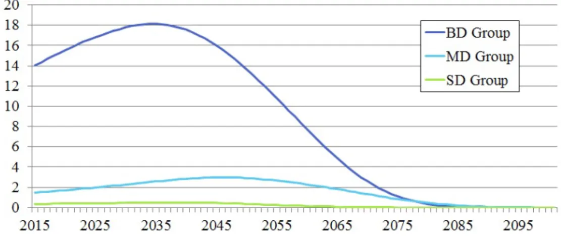
Figure 3.1: Liabilities yearly cash-flows in million euros
These are the cash-flows which were later used to build Matching Portfolios and to compute Technical Provisions and SCR.
3.2
Assets portfolio
There were two main goals for this analysis. Firstly, we wanted to understand the portfolio’s composition and main features and, secondly, we wanted to know if the assets matched the liabilities, i.e., if, at any given year, the nominal value of liabilities was equal to the nominal value of assets, which is a requirement for the MA’s application. From the first part of the analysis, we drew the following conclusions:
General portfolio composition - All portfolios are majorly composed of sovereign
Bonds’ coupon type - The most common coupon type is the fixed coupon (all groups have more than 90% of this type), which pays a fixed coupon amount. The other two material types are the floating coupon, where the coupon de-pends on a money-market index, and the variable coupon, where the coupon depends on other indexes or specified formulas which are based on market conditions.
Bonds’ maturity type - The BD group is again the more diverse, with 83% of
the ”at maturity” type (the plain vanilla bonds) and both callable (the issuer has the option of early redemption) and puttable (the holder has the option of early redemption) types still material but below 6%. The MD group has 99% of ”at maturity” bonds and the SD group has 95% of ”at maturity” and a material amount of callable bonds.
Bonds’ actuarial basis - This is the day count convention used to accrue interest.
The most common is the ACT/ACT with all groups with more than 88%. Both ISMA-30/360 and ACT/360 are material.
Bonds’ Credit Quality Step (CQS) - This is a Solvency II convention that
char-acterizes the credit worthiness of assets. It is an integer scale from 0 to 6 where the lower the CQS, the higher the rating. More information on this mapping can be found at (Joint Committee, 2015). The BD group has an average CQS of 4.10, the MD group has 2.86 and the SD group has 3.37.
Bonds’ yield - The BD group has an average bond yield of 1.9930, the MD has
1.4114 and the SD has 1.1927. For this analysis, for obvious reasons, we excluded bonds with variable and floating coupons.
MA eligibility - Within ”Carteira 5”, the assets eligible for the MA’s application
are bonds (Corporate and Sovereign) with fixed cash-flows (mainly fixed and zero-coupon) which allow no options for issuers. In the BD group these as-sets correspond to 57.67% of the total portfolio, while in the MD group they correspond to 91.64% and in the SD group correspond to 62.75%.
eligible assets. Knowing the bonds’ coupon yield, coupon type, frequency, maturity date and redemption amount, we built the payoff matrix C ∈ Mn×m, where each row corresponds to the cash-flows of a specific bond and each column corresponds to the cash-flows of a specific year. We made some assumptions for simplicity:
• To project the liabilities, we assumed that they were paid in the beginning of
each year. Therefore, in order to be coherent, we discounted all cash-flows of a certain year to the beginning of that year using the forward rates related to the risk-free interest rates published by EIOPA. In this way, the payoff matrix represented the value of assets’ cash-flows at the beginning of each year.
• Since the ACT/ACT was the actual basis more frequent, we used it for all
bonds.
With the payoff matrixC and the column vector wcontaining the number of units invested in each bond1
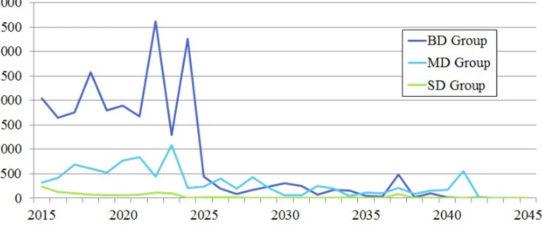
, the annual assets cash-flows were simply the row vectorCw. The results are shown in Figure 3.2.
Figure 3.2: Assets yearly cash-flows in million euros
Once again, the BD group presents higher values in its cash-flows than the other groups. However, the gap between them is lower in this case. Also, assets’ cash-flows are much more irregular and concentrated in earlier years than the liabilities’ cash-flows.
Matching Adjustment Application
4.1
Eligibility criteria
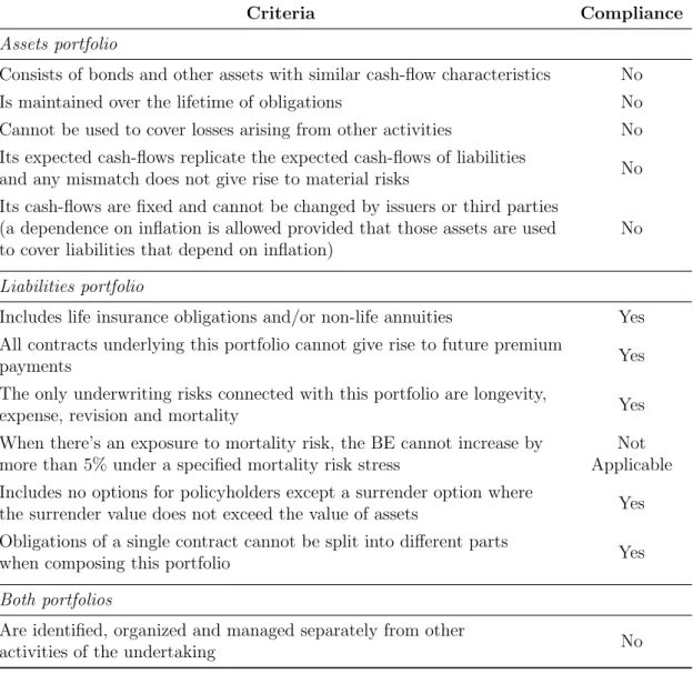
In order to apply the MA to specific portfolios of assets and liabilities, they need to comply a set of criteria defined in the amendment made to the Solvency II Directive by the European Parliament and Council (2014), the Omnibus II Directive. For each group of undertakings (BD, MD and SM), we checked the fulfillment of all criteria and, in the end, all groups failed the same requirements. Indeed, this outcome was expected as undertakings have no reason to adapt their asset portfolios to comply with such criteria in the current regime. The results for all groups are summarized in Table 4.1.
In general, all criterion related with the liabilities portfolio is satisfied because the nature of the D&D pensions’ business in Portugal fits perfectly within the scope of the MA. It includes non-life annuities only exposed to the underwriting risks of longevity, expenses and revision, and such that no future premium payments are generated by them. However, the same does not happen with the assets portfolio, since it fails every criteria. First of all, the portfolio ”Carteira 5” is used to cover all WC liabilities, which disagrees with the requirement setting that assets cannot be
used to cover losses from other activities. Also the aforementioned portfolio is very diversified, including investment in stocks and properties, which are asset types not allowed for the MA’s application. Then, considering only the investment on bonds, there are material investments in floating and variable coupon bonds, which fails the criteria requiring assets with fixed cash-flows. Finally, if we only used the eligible types of assets in the assets portfolio, it would not replicate the liabilities’ cash-flows because there’s a huge gap between the maturities of the two portfolios. Actually, all assets mature before 2044, while liabilities ultimately run past the year 2100.
Criteria Compliance
Assets portfolio
Consists of bonds and other assets with similar cash-flow characteristics No Is maintained over the lifetime of obligations No Cannot be used to cover losses arising from other activities No Its expected cash-flows replicate the expected cash-flows of liabilities
and any mismatch does not give rise to material risks No Its cash-flows are fixed and cannot be changed by issuers or third parties
(a dependence on inflation is allowed provided that those assets are used to cover liabilities that depend on inflation)
No
Liabilities portfolio
Includes life insurance obligations and/or non-life annuities Yes All contracts underlying this portfolio cannot give rise to future premium
payments Yes
The only underwriting risks connected with this portfolio are longevity,
expense, revision and mortality Yes
When there’s an exposure to mortality risk, the BE cannot increase by more than 5% under a specified mortality risk stress
Not Applicable Includes no options for policyholders except a surrender option where
the surrender value does not exceed the value of assets Yes Obligations of a single contract cannot be split into different parts
when composing this portfolio Yes
Both portfolios
Are identified, organized and managed separately from other
activities of the undertaking No
Therefore, we conclude that the market is not yet prepared to apply this measure. Nevertheless, we still want to estimate what would be the MA’s impact in the Portuguese market, assuming it could indeed be applied. Since the problem resides in the assets portfolio, we can build eligible assets portfolios for the market’s real liabilities portfolios and continue the analysis from there.
4.2
Building eligible assets portfolios
The process of building eligible portfolios of assets consisted of three main steps:
1. Find a set of eligible assets with maturities ranging from 2015 to 2074; 2. Select one asset for each different maturity year depending on specified criteria; 3. For each asset, compute the amount of units that should be held in order to
replicate the liabilities’ cash-flows.
Our aim was to build portfolios as close as possible to the real portfolios the un-dertakings already held and to use always real assets being traded in the market by the end of 2014. Thus, for step one, we gathered all eligible assets from the original portfolios and, for maturities not present in those portfolios, we added all eligible assets quoted in Bloomberg and exchanged in euro currency. In the end, we had 3 sets of eligible assets, one for each specific group of undertakings.
For step two, we considered two distinct investment strategies - the portfolio with the highest yield and the portfolio with the highest rating. The first is quite obvious - for each maturity we chose the assets with the highest yield to maturity computed from the 31st of December, 2014. For the second, we didn’t use the assets’ rating, but instead their CQS. For each maturity, we chose the asset with the lowest CQS and, to break a tie, we chose the asset with the highest yield.
Considerndifferent bonds, with market pricesB1, B2, ..., Bn, and their payoff matrix
defined asC= [cij]n×n, where cij is the cash-flow of bondiat timetj. Consider also the liabilities vectorL= [lj]n×1 where lj is the expected liabilities cash-flow at time
tj. Now, for the portfolio w= [wi]n×1, where wi is the number of bondsi held in it, we have that the vector of the assets cash-flows is given by wTC.
The condition is both liabilities and assets having the same cash-flows at all times. Thus w has to be such that wTC = LT
, which is equivalent to wT = LT C−1
if and only if C is invertible. Since both investment strategies define portfolios with exactly one asset per maturity year, from 2015 to 2074, the payoff matrix C is lower triangular, which implies that Cis invertible. Therefore, wT =LTC−1
is the portfolio that perfectly matchesL.
However, this method has some drawbacks and thus some adjustments were made:
• As explained in chapter 3, liabilities’ cash-flows were computed assuming all
pensions were paid at the beginning of the year. However bonds can mature at any time during the year. Since we need the assets first to be able to pay the liabilities, we considered that any bond maturing in a certain year would be used to cover the cash-flows of the next year. For instance, all bonds maturing in 2015 will be used to cover the liabilities of 2016.
• Although liabilities run past the maturity year 2100, the current market does
not contain eligible assets with so long maturities. Therefore, to solve this issue, we considered that the highest maturity year would be 2075 and the assets maturing in that year would have to cover all future liabilities cash-flows. In other words, we added the nominal value of all cash-flows being paid after the year 2075 and assigned that value to the year 2075.
• Although one can only hold an integer number of bonds, this method may lead
to non integer values for wi. In these cases, we rounded the value obtained to
mismatch between the assets and liabilities cash-flows, the mismatch was not material.
• The method may also lead to negative values of wi, which is not acceptable.
In these cases, we considered wi to be zero. Again, the approximation leads to
mismatches. However, the only portfolios where we had to apply it were the two covering the MD group and even in those the mismatch was not material.
Finally, when valuing assets’ cash-flows for applying and computing the MA, the Directive states that those cash-flows must be adjusted to take into account the risk of default. In particular, ˜cij = cij ·(1−PDi) + 0,3·cij ·PDi
1
, where PDi is the
probability of default for bondi, which is provided by EIOPA and depends on the bond’s CQS, maturity and type of issuer (i.e., whether it is Governmental, Financial or Non-financial). Thus, the payoff matrix C was adjusted in step 3 according to the presented formula.
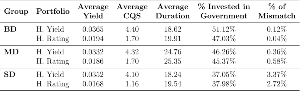
In the end, after implementing the entire process in Excel using functions pro-grammed in VBA, we built 6 different eligible portfolios (two for each group of undertakings), that match the correspondent cash-flows of liabilities. The full con-tent of these Matching portfolios is in Appendix B and their general features are presented in Table 4.2.
Group Portfolio Average Yield
Average CQS
Average Duration
% Invested in Government
% of Mismatch
BD H. Yield 0.0365 4.40 18.62 51.12% 0.12%
H. Rating 0.0194 1.70 19.91 47.03% 0.04%
MD H. Yield 0.0332 4.32 24.76 46.26% 0.36%
H. Rating 0.0186 1.70 25.35 45.37% 0.58%
SD H. Yield 0.0352 4.10 18.24 37.05% 3.37%
H. Rating 0.0168 1.16 19.54 37.98% 2.72%
Table 4.2: Information on Matching portfolios’ general features
4.3
Matching Adjustment computation
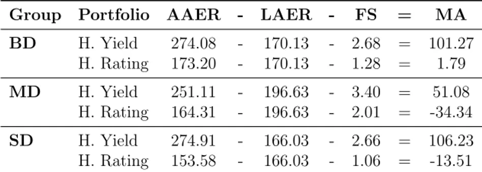
In the Directive’s amendment by European Parliament and Council (2014), the Omnibus II Directive, the MA is defined to be the difference between two annual effective rates, the Assets Annual Effective Rate (AAER) and the Liabilities An-nual Effective Rate (LAER), minus the portfolio’s Fundamental Spread (FS). The directive outlines these concepts as:
AAER - The annual effective rate, calculated as the single discount rate that,
where applied to the cash-flows of the portfolio of insurance or reinsurance obligations, results in a value that is equal to the market value of the portfolio of assigned assets.
LAER - The annual effective rate, calculated as the single discount rate that, where
applied to the cash flows of the portfolio of insurance or reinsurance obligations, results in a value that is equal to the value of the BE of the portfolio of insurance or reinsurance obligations.
Fundamental Spread- the sum of two credit spreads, the one corresponding to
the probability of default of assets and the one corresponding to the expected loss resulting from downgrading of the assets. Both spreads and the FS are provided by EIOPA and depend on the assets’ CQS, maturity and type of issuer. Moreover, the FS used to subtract from the MA must include only the portion of the FS that has not already been reflected in the adjustment to the cash-flows of the assigned portfolio of assets. And finally, the FS of each asset must be at least 30% (for exposures to Member States’ central governments and central banks) or 35% (for any other exposures) of the correspondent long-term average of spread over the risk-free interest rate. These long-long-term average of spread is also computed by EIOPA periodically.
1. Compute the market value of the Matching portfolio as the sum over all assets of their real market value multiplied by the number of units invested in them,
wi;
2. Compute the BE of the liabilities portfolio as the present value of all liabilities’ cash-flows using the risk-free rate term-structure published by EIOPA;
3. Compute both AAER and LAER, as described in the directive, using the Excel’s add-in named Solver;
4. For each asset, get its FS and credit spread corresponding to the probability of default of assets and compute its remaining FS as the difference of the two; 5. Compute each asset’s duration;
6. Compute the weighted average of the assets’ remaining FS, using the amounts invested in each asset and their duration;
7. Finally, compute the MA as the AAER minus the LAER and minus the weighted average remaining FS.
4.4
Remarks and Results
Group Portfolio AAER - LAER - FS = MA
BD H. Yield 274.08 - 170.13 - 2.68 = 101.27 H. Rating 173.20 - 170.13 - 1.28 = 1.79
MD H. Yield 251.11 - 196.63 - 3.40 = 51.08 H. Rating 164.31 - 196.63 - 2.01 = -34.34
SD H. Yield 274.91 - 166.03 - 2.66 = 106.23 H. Rating 153.58 - 166.03 - 1.06 = -13.51
Table 4.3: MA and relevant spreads for its computation, in basis points (1 basis
point equals 0.0001)
Also, there are evident differences between the three groups of undertakings. Firstly, the MD group seems to have a generally lower MA than the other groups, not only due to higher FS’s, but also due to higher LAER’s and, in some cases, lower AAER’s. Secondly, the SD group presents a higher variation between the Highest Yield and Highest Rating portfolios, variation which is experienced both in the AAER and the FS.
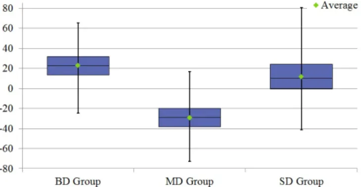
However, are these phenomena happening just in these 6 portfolios or are some trends caused by intrinsic features of the groups and their sets of eligible assets? Also, in broader approach, what impact do the portfolios’ specific features have in the value of the MA? In order to answer these questions, we tried to characterize the distribution of the MA. We already had a Excel workbook that automated the process of computing the MA and thus we changed it to include two functions:
1. Similarly to the functions that find the Highest Yield and Highest Rating portfolios, we build a function that finds a random portfolio.
2. To be able to capture the distribution of the measure, we would have to com-pute it for many random portfolios. Thus, we build an iterative function that runs the MA’s computation process for 1000 random Matching portfolios and stores that information in a Excel spreadsheet.
Figure 4.1: General distribution of the MA, in basis points, per group
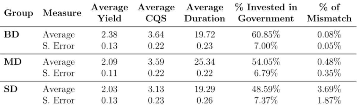
4.4 and 4.5 present the average values and the standard error of all major portfolio’ features and all relevant figures influencing the MA’s calculation.
Group Measure Average Yield
Average CQS
Average Duration
% Invested in Government
% of Mismatch
BD Average 2.38 3.64 19.72 60.85% 0.08%
S. Error 0.13 0.22 0.23 7.00% 0.05%
MD Average 2.09 3.59 25.34 54.05% 0.48%
S. Error 0.11 0.22 0.22 6.79% 0.35%
SD Average 2.03 3.13 19.29 48.59% 3.69%
S. Error 0.13 0.23 0.26 7.37% 1.87%
Table 4.4: MA distribution’s general features
Group Measure AAER - LAER - FS = MA
BD Average 194.75 - 170.13 - 2.12 = 22.50 S. Error 13.54 0.00 0.71 13.95
MD Average 170.28 - 196.63 - 3.12 = -29.46 S. Error 13.20 0.00 0.91 13.91
SD Average 179.74 - 166.03 - 2.09 = 11.63 S. Error 18.93 0.00 0.77 19.30
Table 4.5: MA distribution and relevant spreads, in basis points
Analyzing all the data in detail, we conclude the following:
• The MD group shows a consistently lower MA when compared with the other
groups. This is caused by the particular features of the portfolio, particularly, its longer maturities and low yields.
• The SD group experienced the higher MA’s standard error, which corroborates
the initial suggestion of higher variation. The same happens for almost all its portfolio’s features.
• The AAER expresses the assets portfolios’ yield. Thus, higher average yields
was particularly the case of the Highest Yield portfolios of the groups BD and MD.
• Since the method doesn’t change the value of liabilities, the LAER is constant.
Thus, the initial trend is maintained, where the average SD portfolio has the lowest LAER, followed by the BD’s and finally the MD’s. This spread corre-sponds to the single rate which, when discounting the corresponding liabilities, is equivalent to the risk-free rates published by EIOPA. Thus, the LAER can be acknowledged as the ”liabilities’ maturity-weighted” average of the risk-free rates, which implies that longer tails in the liabilities cash-flows lead to higher LAER’s (the higher the maturity date, the higher is risk-free rate). Indeed, this is consistent with the work developed in Chapter 3, in which the SD group showed the smallest tail, followed by the BD group and the MD group.
• In terms of the FS, the MD group has the highest average, followed by the BD
group and then the SD group (although the BD and SD groups are very close and, in some cases, the BD group has lower FS’s). The measure is complex and many portfolio’s features have impact on its value. Firstly, assets with longer maturities have higher risks of default and downgrade, and thus higher FS’s. Secondly, assets with high credit worthiness are considered less risky and so have generally lower FS’s (lower CQS leads to lower FS’s). The same happens with the investment in central Government and central banks debt -is -is considered less r-isky and has generally lower FS, which helps explain why the BD group has a lower average FS than the MD’s and, at the same time, a higher average CQS.
• The percentage of mismatch remains acceptable. Furthermore, the average SD
Quantitative Impact
5.1
Best Estimate
Under the Solvency II regime, all undertakings have to hold enough assets to cover all Technical Provisions, and thus, changes in the value of Technical Provisions have implications in the undertakings’ solvency position. This is the relevance of the BE, which is the part of Technical Provisions that corresponds to the expected present value of all future cash-flows. The cash-flows include premiums, benefits, expenses, and so on. However, in our case, we only considered benefits because the D&D liabilities portfolios do not include material expenses nor premium payments. Thus, in order to compute the BE, we just needed the liabilities cash-flows and the relevant interest rate term structure.
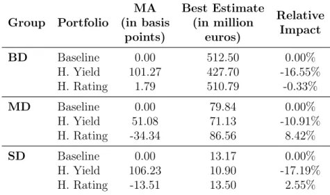
In Chapter 3, we computed the liabilities’ yearly cash-flows since 2015 and, in Chap-ter 4, we computed the value of the MA’s for all six portfolios. Then, we computed the adjusted interest rate as the MA plus the relevant risk-free interest rate term structure published by EIOPA. For each group of undertakings, Table 5.1 describes the values of the BE for the two portfolios constructed in chapter 4 and for a situation without the application of the MA, which is identified as the baseline.
Group Portfolio
MA (in basis
points)
Best Estimate (in million
euros)
Relative Impact
BD Baseline 0.00 512.50 0.00%
H. Yield 101.27 427.70 -16.55% H. Rating 1.79 510.79 -0.33%
MD Baseline 0.00 79.84 0.00%
H. Yield 51.08 71.13 -10.91% H. Rating -34.34 86.56 8.42%
SD Baseline 0.00 13.17 0.00%
H. Yield 106.23 10.90 -17.19% H. Rating -13.51 13.50 2.55% Table 5.1: Quantitative impact in the Best Estimate
As expected, there’s a direct relation between the MA and the impact of its appli-cation in the BE - the higher the MA, the lower the BE and the more favorable it is for an undertaking. In fact, the higher the MA, the higher is the interest rate term structure and consequently the lower is the liabilities’ present value. Also, a negative value in the MA generates an increase in the BE, which is disadvantageous for the undertaking.
The more favorable impact can be seen in the Highest Yield portfolios, with a decrease in the BE varying between 17,19% and 10,91%, while in the Highest Rating portfolios there’s a variation from -0,33% to 8,42%. This fact seams to indicate that, for the purpose of building the Matching portfolios, choosing profitability over security would be preferable. Nevertheless, the impact on the SCR may revert this scenario.
5.2
Solvency Capital Requirement
The SCR is the measure corresponding to the capital needed to sustain a shock corresponding to the 99.5% value-at-risk for an one year time horizon. Undertakings have to compute their SCR at least once a year and should hold enough Basic Own Funds (BOF) to fully cover that value. Therefore, changes in the SCR’s value have implications in the undertakings’ solvency position.
In order to compute the SCR, undertakings are given two options - either use the SCR standard formula set out in the Directive or use an internal model, which is a formula built by the undertaking and approved by the supervisory authority. For the purpose of the quantitative impact analysis, we chose to use the SCR standard formula.
In the standard formula, whose full structure is represented in appendix C, the SCR is computed as the sum of 3 modules, namely the adjustment for the loss absorbing capacity of Technical Provisions and deferred taxes, the operational risk and the Basic SCR. The first two have a specific formula set out in the Delegated Acts, while the Basic SCR is itself divided into 6 modules, some of them divided into sub-modules. Each module/sub-module represents a specific risk an undertaking may be exposed to and its calculation is based on the impact of a stressed scenario in the BOF. All stressed scenarios are set as specific shocks calibrated at European level to reflect the aggregated 99.5% value-at-risk for the one year time horizon. In particular, the basic SCR is computed through the following steps:
1. The whole balance sheet is valued in normal conditions, using proper methods based on market consistent principles. The BOF are computed as the excess of assets over liabilities, taking into account the eligible subordinated liabilities. 2. Given a specific module/sub-module, a shock relating the risk considered in
stressed BOF item is again computed. During the revaluation, the Risk Mar-gin is assumed not to change and the loss-absorbing capacity of Technical Provisions and deferred taxes is not accounted for.
3. The capital charge for that module/sub-module is computed as the difference between the normal conditions’ and the stressed BOF. Negative variations in BOF are recognized as positive capital charges. If the variation in BOF has a positive sign, then the capital charge is set to zero.
4. After the capital charges for all shocks are computed, they are aggregated assuming Normal distributions and using linear correlation matrices published in the Delegated Acts (European Commission, 2014).
The SCR is a very complex and sophisticated formula, built to quantify all the risks to which an undertaking is exposed to. It is not the purpose of this thesis to go into much detail on this topic. Therefore, we tried to simplify the computation as much as possible, always taking into account that the end-goal is to compute the impact of applying the MA to a general Portuguese undertaking.
5.2.1
SCR in Matching Adjustment Portfolios
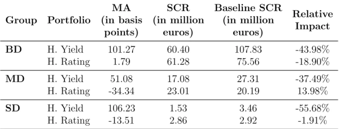
As before, we built an Excel workbook which includes VBA programmed functions in order to make the calculations as automated as possible. We also computed two SCR’s for each portfolio - one considering application of the MA and another not considering it, which we called the baseline portfolio. Table 5.2 resumes the computed values and the relative impact of the MA’s application.
Group Portfolio MA (in basis points) SCR (in million euros) Baseline SCR (in million euros) Relative Impact
BD H. Yield 101.27 60.40 107.83 -43.98% H. Rating 1.79 61.28 75.56 -18.90%
MD H. Yield 51.08 17.08 27.31 -37.49% H. Rating -34.34 23.01 20.19 13.98%
SD H. Yield 106.23 1.53 3.46 -55.68%
H. Rating -13.51 2.86 2.92 -1.91% Table 5.2: SCR for MA Portfolios and corresponding baselines
The results indicate that there’s a benefit in terms of SCR when applying the MA, since almost every portfolio had a reduction in their SCR’s, even the SD group’s Highest Rating portfolio, which has a negative MA. This impact is more accentu-ated in the Highest Yield portfolios and indicates that higher values of MA lead to more beneficial impacts. Moreover, when computing risk modules based on shock scenarios, we must not take into account the MA and thus the impact here is null. The exception, and reason behind the reduction experienced, is the market spread risk sub-module, which includes a specific adjustment in case of applying the MA. This is logical and expected, since, as discussed earlier, the criteria to build eligible MA portfolios mitigates the risk of losses due to spread fluctuations.
5.2.2
Approximation for an undertaking applying the MA
analyzed the impact of applying the MA only on those portfolios. However, no undertaking deals exclusively on D&D pensions and thus, to fully access this impact, we need to consider the rest of the undertaking’s business. Specially in terms of the SCR, because there’s a loss of diversification benefits, analyzing the entire business may lead to different conclusions.
In order to perform this analysis, we used data from the quantitative report for the preparatory phase of Solvency II carried out by ASF in the Portuguese insur-ance market, which included the value and computation of each undertaking’s SCR. However, due to many problems with the reported data, we had to exclude some companies from the initial sample set. In particular, for both MD and SD groups, we ended with just one undertaking, which is considered to represent well the group and has an acceptable report quality. Then, for the BD group, we considered all undertakings and thus, we aggregated each specific SCR’s sub-module by taking the weighted average according with the market shares. The goal here was to adapt the sub-modules’ reported values to simulate the application of the MA in an undertak-ing and, for that, we had to make some assumptions, namely:
• In a real situation, an undertaking intending to apply the MA and who does
not have an asset portfolio which replicates the correspondent liabilities, has to buy new assets that meet all the requirements. Thus, to simulate this trade, we chose EU government bonds with fixed cash-flows from the undertaking’s original assets portfolio, which, when sold at their quoted market value in the end of 2014, were enough to buy the correspondent Matching portfolio. In terms of the rest of the business’ SCR, this sale only affects the interest rate and the concentration sub-modules, although in the case of the concentration sub-module, the sale would be likely immaterial and reduce the capital charge. Therefore, we only considered the impact of the sale in the interest rate risk sub-module.
• The lines of business incorporated in the SLT health underwriting risk
assistance. However, in the Portuguese market, the second is so much less significant than the D&D pensions that we can consider it immaterial. Thus, in terms of the rest of the business’ SCR, we assume that removing this sub-module would be same as removing the exact underwriting risks related with the D&D pensions’ liabilities portfolio.
And finally, the method used was the following:
• Collect the value of each SCR Standard Formula’s module or sub-module; • Annul the SLT Health sub-module and subtract the amount of the interest
rate risk sub-module corresponding to assets chosen to be sold in exchange for the Matching portfolio;
• Aggregate the resulting modules/sub-modules according with the Standard
Formula’s rules, obtaining the henceforth called SCR of the rest of the business;
• Add the SCR of the rest of the business with the SCR of the Matching portfolio,
obtaining the final SCR with the application of the MA.
5.3
Final results and remarks
5.3.1
General impact of the Matching Adjustment
In order to measure the impact of applying the MA in an undertaking, we chose 3 metrics relating with an undertakings’ available assets, risk exposure and solvency position. Respectively, they are:
Basic Own Funds - Using again the quantitative report for the preparatory phase
Then, to compute this measure after the application of the MA, we subtracted the impact observed in the BE from Table 5.1, adjusted to take into account the increase in deferred taxes. The formula was:
BOFaf terM A =BOFinitial−(BEaf terM A−BEinitial)(1−0.23) (5.1)
SCR - All the computations were already done here. We used the initial SCR of
each group and their final SCR including the application MA.
Solvency Ratio - This ratio measures the solvency of an undertaking, that is, its
ability of meeting future liabilities. It is computed as the ratio of BOF to cover the SCR over the SCR itself.
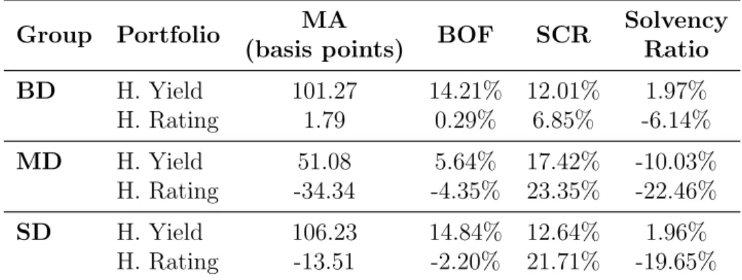
The relative impact on the three metrics is presented in Table 5.3.
Group Portfolio MA
(basis points) BOF SCR
Solvency Ratio
BD H. Yield 101.27 14.21% 12.01% 1.97% H. Rating 1.79 0.29% 6.85% -6.14%
MD H. Yield 51.08 5.64% 17.42% -10.03% H. Rating -34.34 -4.35% 23.35% -22.46%
SD H. Yield 106.23 14.84% 12.64% 1.96% H. Rating -13.51 -2.20% 21.71% -19.65% Table 5.3: Relative impact on solvency of the Matching Adjustment
And finally, the main conclusions are the following:
• First of all, it is clear that the higher the value of the MA, the higher is the
• In terms of the SCR, the groups were always penalized for applying the MA.
Despite the reduction in the market’s spread risk submodule, the loss of di-versification benefits when applying the MA caused the SCR to increase in every portfolio, which implies an increase in the assets allocated to sustain unexpected losses.
• On one hand, the MA was beneficial because it increased the undertaking’s
available capital. Yet, on the other hand, the MA was disadvantageous because it increased the capital needed to sustain unexpected losses, which decreased the accessible capital an undertaking has to expand and/or create new business. This duality is the reason why we chose to analyze the solvency ratio -since it balances both BOF and SCR, it represents the general impact in an undertaking. According to this metric, there are only two portfolios where it was advantageous to apply the MA. They are the BD and SD groups’ Highest Yield portfolios. In these portfolios, the relative increase in own funds was higher than the relative increase in the SCR, which led to an improvement in the solvency position of the undertaking.
5.3.2
General impact of the Volatility Adjustment
The last goal proposed to the internship was to compare the MA with other LTG measures, in particular, the Volatility Adjustment (VA). This measure was built by EIOPA to mitigate pro-cyclical investment behaviors when markets deteriorate due to wide bonds’ spreads and bonds’ low liquidity. The VA is a risk-corrected spread which is added to the risk-free interest rate term structure used to discount Technical Provisions and is calculated based on reference portfolios for each currency.
Similarly to the MA, we assessed the impact of applying the VA on three items - the BOF, the SCR and the Solvency ratio. The results are summarized in Table 5.4.
Group BOF SCR Solvency Ratio BD 2.26% 0.00% 2.26% MD 1.94% 0.00% 1.94% SD 2.56% 0.00% 2.56%
Table 5.4: Relative impact on solvency of the Volatility Adjustment
In terms of the BOF, the impact was computed using formula 5.1, where the index
”MA” is replaced by ”VA”. Similarly to the MA, because there’s a rise in the interest rates used to discount Technical Provisions, when applying the VA, the BE decreases, which increases the value of Own Funds and results in a favorable impact for the undertaking. Secondly, in terms of the SCR, the measure has no impact on the standard formula’s modules computed by stressed scenarios and thus, for every group of undertakings, the impact observed in the SCR was null and the impact experienced in the Solvency Ratio is same as the BOF’s.
Conclusion
The work developed during my internship at ASF was aimed to assess the impact of applying the MA in a specific line of business in Portugal - the Workers’ Compensa-tion insurance. In particular, we focused on the Death and Disability pensions due to their features, which are well suited for applying the MA.
In order to better represent the market, we decided to divide all undertakings with business in WC insurance and supervised by ASF in 3 groups, according with their market shares – the BD group represented 81% of the market, the MD group had 17% of the market and the SD group constituted 2% of the market. In fact, we considered the market shares weighted average of each group’s undertakings, creating thus notional undertakings that were representative of the respective groups. Then, using the 3 groups, we did a series of computations and analysis based on real data reported to ASF. Our main conclusions were the following:
• As expected, the current WC insurance market is not yet prepared to apply
the MA since the assets portfolios don’t fulfill the mandatory criteria and the liabilities and assets cash-flows are not matched at all times (assets cash-flows are higher the the first maturity years and have much shorter maturities then the liabilities cash-flows).
• The MD group presents generally lower values of MA than the other two
groups, mainly due to its liabilities’ longer tail and its assets’ yields. Also, the BD and SD groups are similar in terms of main portfolio features and MA value. However, the SD group presents a higher variability and higher value of mismatch between assets and liabilities. This is caused by the difference of their liabilities’ dimension.
• In terms of Technical Provisions, the Best Estimate is the component that
experiences the most relevant impact. In fact, there’s a direct relation between the measure and the MA - the higher the MA the lower is the relative value of the Best Estimate and the more beneficial it is for the undertaking.
• Own Funds are directly influenced by changes in Technical Provisions.
Ap-proximately, the BOF are simply the excess of assets over liabilities and, since a decrease in the Best Estimate causes a decrease in liabilities, the higher the value of the MA, the higher are the BOF. Therefore, in terms of BOF, even after the adjustments due to the loss in deferred taxes, we observed an improvement when applying the MA.
• In the case of the SCR, there are two different situations. Firstly, when we
only consider the SCR of the D&D related portfolios, due to the decrease in the spread risk sub-module, the application of the MA reduces the value of the SCR, which is beneficial for an undertaking. However, when we look at the global impact in an undertaking, the application of the MA increases the value of the SCR, because the benefit in the spread risk sub-module isn’t high enough to offset the loss of diversification benefits. Thus, in terms of the SCR, applying the MA is disadvantageous for an undertaking.
• In order to measure the global impact of applying the MA in an
the Matching portfolio, an undertaking should choose profitability over credit quality, which appears to be counter-intuitive. Nevertheless, the use of the MA in each portfolio has to be approved by the supervisory authority and thus, in practice, an undertaking will have to guarantee a certain degree of safety in credit worthiness. Also, the measure appears to be more beneficial to either undertakings with a large business or to undertakings with an very representative WC business, since, in both cases, the loss in diversification benefits would be relatively lower.
• Finally, in the current market conditions, the impact of applying the VA is
more favorable in every group of undertakings than the impact of applying the MA. However, this result doesn’t mean that the VA is always more favorable than the MA, since it is very dependent on market conditions and can be only applied in specific cases where the markets are unstable.
Clearly, applying the MA can be advantageous to an undertaking. However, due to the fact that, once applying the measure, an undertaking cannot revert back to not applying it, it’s essential to do a complete study of the MA’s behavior in the specific undertaking under various market scenarios. Also, the results indicate that in undertakings with a similar profile to the MD group it wouldn’t be advantageous to apply the MA. Nonetheless, the MA is so tailor-made that small differences in the undertaking’s business and in the D&D portfolios may cause huge differences in the final impact. Therefore, an interesting development of this work would be to focus on a specific Portuguese undertaking and do a thorough analysis.
Technical Specification for the
Liabilities Portfolio
A.1
Annual aggravation rates
Table A.1 contains the percentage of revisions on D&D pensions observed in the data corresponding to years 2012, 2013 and 2014, contains the average percentage of the pension’s aggravation, in case a revision has occurred, and the final aggravation rate, which is give by the product of the two.
Percentage
of revisions Average Aggravation Aggravation rate
Year 2012 2013 2014 2012 2013 2014 2012 2013 2014
Disability
Revision 2,89% 3,49% 2,55% 54,19% 54,55% 22,09% 1,57% 1,90% 0,56% State change
to Definitive 2,29% 2,46% 2,57% 10,08% 21,39% 20,83% 0,23% 0,53% 0,54%
Total 5,18% 5,95% 5,12% 64,27% 75,94% 42,92% 3,33% 4,52% 2,20%
Table A.1: Aggravation Analysis