A decision support system for the production scheduling of a printing plant

(1)

A Decision Support System for the

Production Scheduling of a Printing Plant

Horácio Magalhães Neri

Master’s Dissertation

Supervisor: Bernardo Sobrinho Simões de Almada-Lobo Co-supervisor: Luís Gonçalo Rodrigues Reis Figueira

Mestrado Integrado em Engenharia Industrial e Gestão

(2)

(3)

Abstract

Pressured by an increasingly competitive global market, production companies are more con-cerned than ever with operational optimization. One of the typical tasks performed in this type of companies is the production scheduling. Even for simple environments, scheduling tasks are known to be complex combinatorial problems. In a printing plant, the problem is especially com-plex due to its large flexibility. Contrarily to common scheduling problems, in a printing plant, the number of operations required to complete a job is not pre-defined.

Motivated by a real-world case of a Portuguese metal-sheet packaging company, a decision support system is developed to support the production scheduling of the printing plant. The de-cision support system is not just an optimization tool. It is designed to increase the efficiency of upstream and downstream processes by providing longer-term information, and also to allow making what-if analysis that can influence tactical-level decisions.

In this dissertation, the problem is decomposed into four subproblems to decrease the com-putational time required to find a solution. Firstly, the bottleneck stage is tackled separately from the other stages. Secondly, for each of the resulting subproblems, the machine assignment is done before the sequencing process. Every subproblem is solved with the aid of mixed-integer linear programming models.

Additional analysis of the current planning process of the company is also presented. This analysis aims to find improvement opportunities and also to address the lack of stored data related to some important parameters of the decision support system. Different concepts and techniques are used during this analysis, such as multiple linear regressions and the overall equipment effi-ciency.

At the end of this dissertation project, the validation of the results had not been completed. However, the solutions analyzed are motivating, since they show that the requirements of the problem are being met and that the information provided by the decision support system meets the company’s needs.

(4)

(5)

Resumo

Pressionadas por um mercado global cada vez mais competitivo, as empresas industriais, mais do que nunca, procuram soluções de optimização operacional. Uma das tarefas típicas neste tipo de empresas é o escalonamento da produção. Mesmo em ambientes de pouca complexidade, o escalonamento é uma tarefa combinatória complicada. Numa fábrica de impressão, o problema é ainda mais complexo devido à sua grande flexibilidade. Ao contrário dos problemas de escalon-amento comuns, numa fábrica de impressão, o número de operações necessárias para completar um trabalho não está previamente definido.

Motivado por um caso real de uma empresa de embalagens metálicas Portuguesa, um sistema de apoio à decisão é desenvolvido para ajudar o escalonamento da produção na fábrica de im-pressão. O sistema de apoio à decisão não será só uma ferramenta de optimização, mas tambem deverá permitir fazer análises de cenários para servir de apoio a decisões táticas.

Nesta dissertação, o problema é decomposto em quatro subproblemas para diminuir o esforço computacional necessário para chegar a uma solução. Primeiro, o gargalo do sistema é abordado em separado dos outros estágios. Segundo, para cada um dos subprblemas resultantes, a fase de alocação das tarefas às linhas de produção é processada antes da fase de sequenciamento. Todos os subproblemas são resolvidos através de modelos de programação linear inteira mista.

Também são apresentadas análises feitas ao atual processo de planeamento para encontrar possíveis oportunidades de melhoria, e para colmatar a falta de dados relacionados com parâmet-ros importantes para o sistema de apoio à decisão. São utilizados diferentes conceitos e técnicas durante estas análises, como por exemplo, regressões lineares múltiplas e a eficácia global dos equipamentos.

Na data de conclusão desta dissertação, a validação de resultados ainda não tinha sido con-cluída. Contudo, as soluções analisadas até ao momento são motivadoras, visto que mostram que os requisitos do problema estão a ser cumpridos e que a informação disponibilizada pelo sistema de apoio à decisão vai de encontro às necessidades da empresa.

(6)

(7)

Acknowledgments

First, I would like to thank my supervisor, Prof. Bernardo Almada-Lobo for the opportunity to work with him in such a challenging project. His expertise and experience were crucial to define the direction of the project and to help me grow, not only as a professional, but also as a person.

I would also like to thank Prof. Gonçalo Figueira, who closely followed the progress of the project. He helped me solve the many obstacles that appeared along the way. More than a co-supervisor, he has been a friend. As the project team is concerned, I would also like to address a word to Prof. Luís Guimarães, whose knowledge concerning operations research is impressive and a great motivation to make me want to improve.

I am also grateful to the team of Colep who gave us the access to the data needed to continue the development of this project and have always shown us confidence in the value of our work.

My colleagues from CEGI, who I met in the first day of this project, and soon became friends, also played a major role on motivating me and offering me wise advice to pursue my goals. Because life is not all about work, I would like to thank my friends from FEUP, and my friends from high school for supporting me when I was in need and for not allowing me to spend the weekends sleeping at home.

Finally, a special "thank you" to my family, mainly my parents and sister. Mãe, Pai, Megui, thank you for always being there when I needed and for helping me getting where I am today.

(8)

(9)

Acronyms and Symbols

AIC Akaike Information Criterion CMYK Cyan, Magenta, Yellow and Black CO Combination of Orders

CP Constraint Programming DSS Decision Support System EDD Earliest Due Date first FCFS First-Come First-Served

FJSSP Flexible Job Shop Scheduling Problem GA Genetic Algorithm

ILS Iterative Local Search KPI Key Performance Indicators LPT Longest Processing Time first MILP Mixed-Integer Linear Programming MP Mathematical Programming

MS Minimum Slack first MTO Make to Order MTS Make to Stock

OEE Overall Equipment Efficiency PAM Partitioning Around Medoids SBH Shifting Bottleneck Heuristic SPT Shortest Processing Time first TS Tabu-Search

VNS Variable Neighborhood Search WIP Work in Process

(12)

(13)

List of Figures

1.1 Schedule of the proposed project . . . 2

2.1 Production stages in the printing plant . . . 5

2.2 Representation of machine M5 . . . 8

2.3 Cutting process in the secondary cut stage . . . 9

2.4 Example of a combination of orders . . . 11

2.5 Example of a CO of 2 orders with three rows per sheet . . . 11

3.1 Disjunctive graph representation . . . 19

4.1 Distribution of time between operations . . . 25

4.2 Time between operations over time . . . 25

4.3 Variation of the average waiting time between stages in lithography . . . 26

4.4 Representation of the overall equipment efficiency (OEE) calculation . . . 27

4.5 Comparison between the real setup time and the estimated setup times in varnish-ing machines . . . 30

4.6 Comparison between the real setup time and the estimated setup times in machine M11 . . . 30

4.7 Rolling horizon scheme implemented in the DSS . . . 32

4.8 Example division of days of the result generated on a Thursday morning . . . 33

4.9 Scheme of the interface of the DSS . . . 33

5.1 Illustrative representation of the different formulations . . . 36

5.2 Scheme of the decomposition of the problem . . . 37

5.3 Example of a small instance for the printing stage . . . 40

5.4 Schematic representation of the machine assignment model for the printing stage 41 5.5 Schematic representation of the sequencing model for the printing stage . . . 44

6.1 Behavior of the value of the objective value and optimality gap in the sequencing phase of the printing stage . . . 50

6.2 Example of a schedule of machine M11 . . . 51

(14)

(15)

List of Tables

2.1 Specialization of varnish machines . . . 7

2.2 Characteristics of the printing machines . . . 7

2.3 Example of possible machine sequences for an order with four colors . . . 8

4.1 Real processing speeds of printing machines . . . 27

4.2 Possible setup time drivers . . . 28

4.3 Results of the multiple linear regression for each machine . . . 29

4.4 Fixed days, detailed schedule and aggregated schedule for each day of the week . 32 4.5 Key performance indicators calculated by the DSS . . . 34

6.1 Comparison of the gaps of each model over time . . . 51

6.2 Example of KPI computed by the DSS . . . 52

(16)

(17)

Chapter 1

Introduction

1.1 Motivation

The increasing complexity of companies and supply chains enlarges the number and the range of decisions to be made. Executives of top tier companies can not decide the future of a com-pany alone without delegating short-term and mid-term planning to other employees. Increasing the number of people involved in the decision-making process creates issues related with the co-herence of the decisions since each individual has different motivations that in some cases may neglect the bigger picture.

Hierarchical Production Planning (HPP), decomposes the overall planning problem into plan-ning modules. Long-term, mid-term and short-term decisions are considered with different levels of detail to balance optimality and practicability. The operational level is the lowest level of de-cisions considered in the HPP. Daily dede-cisions that have a short-term impact on the company are contemplated here. Ordering materials, production scheduling, distribution scheduling, and short-term sales planning are examples of operational decisions.

Despite their short-term impact, operational-level decisions play an important role on the ef-ficiency and effectiveness of the company. Operational optimization is currently becoming more popular, as managers become aware of its potential value. In production environments, production scheduling is a typical short-term planning task that may have a large influence on the throughput of the plant and on customer loyalty by increasing the proportion of orders that meet their due dates.

While forecasting and simulation models are used in predictive analytics, in prescriptive ana-lytics, where the goal is to support the decision making by suggesting possible solutions, optimiza-tion models are applied. Optimizaoptimiza-tion models are often incorporated in decision support systems, which are interactive information systems designed to receive, process and return information in order to aid the decision-making process.

(18)

2 Introduction

1.2 Scope of the Project

The study focuses on a Portuguese company that produces metal packages for different types of products. Metal packages are used by a wide range of sectors from food industry to hygiene products. This variety of sectors increases the spectrum of requirements of customers, demand-ing high levels of customization. As in other sectors, globalization opened new opportunities for growth, but also created new challenges to overcome as the number and economical power of competitors increased. Companies that can not compete in price have to find other competitive advantages such as customization or shorter lead times. To increase their flexibility the customers have been ordering more frequently but in less quantities than what was observed in the past, re-quiring short lead times to be able to fulfill their demand.

The company has several factories spread around Europe, the factory under study is located in Portugal and is divided into two facilities, the printing plant and the metal packaging plant. The focus of the project is the printing plant, more precisely the lithography stage where varnishes and inks are applied to the metal sheets. According to company managers, the lithography phase is the bottleneck of the company, mostly due to the large setup times that are highly dependent on the sequence of operations processed. Currently, scheduling is done manually and relies heavily on the experience of the scheduler.

In an effort to increase the overall throughput of the factory, this project focuses on the bottle-neck of the production process. The company believes that the automation of the process associ-ated with the usage of sophisticassoci-ated optimization techniques will prove to be a major asset in the future. It should be noted that due to confidentiality agreements, some of the values present in this report do not correspond to reality. The schedule of the proposed project is presented in figure 1.1.

(19)

1.3 Dissertation Structure 3

1.3 Dissertation Structure

The dissertation is divided in six chapters that are organized as follows.

The case study is explained in chapter 2. Firstly, the production process in the printing plant is described and secondly, the current scheduling process is analyzed.

In chapter 3 it is possible to find a review of the literature on scheduling problems and common solutions methods used to solve them. The flexible job shop problem is studied in more detail since it is the closest machine environment to the problem under study.

In chapter 4 the decision support system developed is presented. A diagnosis of the current planning process and some analysis on the data that will be used as input to the system are reported. The rolling horizon strategy used to tackle some operational constraints is also explained. Finally, the interface of the system is disclosed, inputs, outputs and KPI are described.

In chapter 5 the decision model is presented. It begins by introducing some of the tested formulations, then the decomposition of the problem is justified and finally, each mathematical model is explained.

Chapter 6 presents the steps taken to validate the solutions generated by the decision support system.

In the last chapter conclusions are drawn and the future direction of the project is disclosed, as well as opportunities to improve the proposed methodology.

(20)

(21)

Chapter 2

The Challenge

This chapter is divided into two sections. In the first section the production process of the printing plant is described, detailing each production stage. In the second section the current scheduling process is depicted.

2.1 Production Process

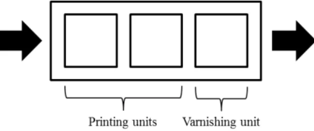
The printing plant, which is the subject of this study, includes the stages illustrated in fig-ure 2.1, namely the primary cut, the lithography and the secondary cut. The focus of this project is the production scheduling of lithography, which includes three main production phases: prepa-ration, printing and finishing. In the first and last phases, varnishes are applied, in the printing stage, colors are printed into the metal sheet. It is also important to understand the requirements of upstream and downstream processes, since they constitute constraints that must be considered when scheduling the lithography stage.

Figure 2.1: Production stages in the printing plant

As mentioned in the first chapter, setup times are a major concern in the printing plant. With clients ordering more times, but in less quantity, more setups are performed. In this paragraph, a brief description of setups is presented, later in chapter 4, a deeper analysis can be found.

In both varnish and printing machines, setup times depend on the previous and the following orders. Setups involve preparing the machine for new sheet formats, changing colors or varnishes, among other operations. The time spent changing these features depends both on the difference

(22)

6 The Challenge

from one operation to the next and on the direction of the changes, since increasing the size of the format takes more time than decreasing, and changing from a dark color to a lighter color takes more time than the opposite. In other words, the setup matrix is asymmetric.

One last remark that is noteworthy is that setups in the printing stage can be split into two phases: static setup and dynamic setup, as named by the company. Static setups involve the operations that have been described so far. Dynamic setups include the adjustments made to ensure that the combination of color results exactly on what the client wants. The times related with this type of setups are highly dependent on the operator and are extremely hard to anticipate.

2.1.1 Primary Cut

The primary cut is the first processing stage in the printing plant. Here, coils are cut into metal sheets that will later be turned into packages of different sizes and formats.

Since raw materials are a major factor on the cost of the final product, sheets with different widths and/or thicknesses are produced using coils with different sizes to reduce waste. It is also important to mention that different coils might require different blades to be cut. There are three types of blades used in this facility: thin, thick and scroll.

The setup times between different coils and sheet formats are not a major concern in this stage, but when blades are changed, the changeover time involved is an issue. To avoid these setups, pro-duction is scheduled to use the same blade as much as possible, with cycles of up to four days.

This stage works in a make-to-stock (MTS) fashion, where production and procurement are based on forecasted demand. This fact, allied with the long production cycles pose a challenge for the next stages since orders that do not have enough sheets ready to be varnished or printed may need to wait a long time to begin production.

2.1.2 Varnishing: Preparation

This production phase involves two main types of operations: application of varnish to the internal side of the sheet and application of varnish to the external side of the sheet. The first is used as a layer of protection between the metal and the contained product, and/or for appearance purposes. The second is used to ensure that the colors printed in the next stage stick to the sheet and/or for appearance purposes as well.

Usually an order involves one internal varnish and one external varnish, but this is not always the case. Some orders need more than one internal or external varnish, and some need more than one application of the same varnish. These requirements are agreed with the client beforehand and when the order is created, the number of operations required in this stage is already given.

There are five machines that can be used to apply varnish, identified in the set {M2, M3, M4, M5, M6}.

Each of these machines can apply one varnish per operation. Even though the machines are ex-tremely flexible, and in theory every machine can process every kind of varnish, in practice, due to the different processing times, some machines are specialized as stated in table 2.1.

(23)

2.1 Production Process 7

Table 2.1: Specialization of varnish machines Machine Varnish M₂ White varnishes M3 Finishing varnishes M4 Golden varnishes M₅ Finishing varnishes M6 Flexible

This is an interesting idea since it takes advantage of machine efficiency, and also decreases the setup times by grouping similar products on the same machines. However, it is important to pay attention to the work load balance and adapt machines that are less demanded to help ma-chines that are not being able to meet the due dates.

As stated previously in this section, varnishes are applied depending on client’s requirements and therefore this stage works mostly under a make-to-order (MTO) policy. However, because some combinations of varnishes are very frequent, some operations are performed in a MTS fash-ion.

2.1.3 Printing

As the name suggests, in this phase of production colors are printed on the metal sheet. The patterns and colors printed depend on the product and client being considered, so, this stage fol-lows a MTO strategy in all cases. Orders have a set of colors that must be performed, and the sequence of colors should also be followed to ensure that the final product is exactly as agreed with the client.

Contrarily to the varnish machines, in the printing stage, machines can print more than one color in the same operation, the number of colors a machine can print depends on the number of printing units it has. Printing machines are identified in the set {M5, M11, M13, M15}, different

characteristics, including the number of printing units of each machine can be seen in table 2.2. Table 2.2: Characteristics of the printing machines

Machine Number of Printing Units Nominal Speed Average Setup Time (min) M₅ 2 6000 sheets/hour 46

M11 4 6300 sheets/hour 74

M13 2 6300 sheets/hour 56

M₁₅ 7 9700 sheets/hour 86

One of the features that makes the printing plant such an interesting case study, and at the same time increases the complexity of the problem, is the fact that the number of operations required to complete each order depends on the machines chosen to process it. In table 2.3 it is presented an example of possible machine sequences for an order with 4 colors.

(24)

8 The Challenge

Table 2.3: Example of possible machine sequences for an order with four colors Printing Stage Number of printing operations

M₅- M5 2 M11 1 M13- M13 2 M₁₅ 1 M13- M5 2 M5- M13 2

At the moment of the project, the maximum amount of colors allowed per order was eight. It is interesting to notice that an order with seven colors can be processed in any number of operations, from one (M15) to four (ex: M5-M5-M5-M5).

Intuitively, it might seem obvious that the best approach is to use machines that minimize the number of operations needed, to decrease the number of setups performed. However, this is not always the case. Since, as explained in the beginning of this chapter, setup times depend on the difference of colors and formats between two consecutive operations, using more operations may be beneficial if they are similar to other operations performed on the same machine.

Jobs can be divided into two main categories depending on the type of colors they require. Some jobs use primary colors (cyan, magenta and yellow) and black to reproduce an almost infinite amount of colors, while others require the application of direct colors to achieve the desired result. To differentiate both types of jobs, they are called CMYK and Pantones, respectively.

2.1.4 Varnishing: Finishing

In the last stage of lithography, one or more finishing varnishes are applied on top of the colors to give a shiny or matte effect and/or to serve as a layer of protection to avoid direct contact between skin and paint.

As seen in subsection 2.1.2, machines M3 and M5 are used to apply finishing varnishes. It is

important to notice that machine M5can also be used to print colors as stated in subsection 2.1.3.

In figure 2.2 it is possible to see that the varnishing unit comes after the printing units, and that is the main reason why M5is used for finishing varnishes instead of preparation. This way, in the

same operation it is possible to print two colors and apply one layer of finishing varnish.

(25)

2.2 Current Scheduling Process 9

2.1.5 Secondary Cut

In the secondary cut phase, sheets are cut into single bodies as explained in figure 2.3. Even though both cuts are made in a single operation, the cut sequence can not be disregarded as will be explained in subsection 2.2.3 due to the fact that every body in the same row of bodies falls into the same container Cxto be taken to the next production stage.

While the previous stages work every day of the week, all day long, the secondary cut does not work during the weekends because it has excess capacity. It is noticeable that at the beginning of the week there are many orders waiting to be cut, while at the end of the week the machines are waiting for jobs to perform. This unbalance creates issues that will be explained in the next section.

Figure 2.3: Cutting process in the secondary cut stage

2.2 Current Scheduling Process

The current scheduling process may be divided into different phases: machine assignment, combination of orders and sequencing. In this section all the phases are described. Furthermore, an initial introduction to the tactical-level planning is presented.

2.2.1 Planning Process

The main decision made in the planning stage are the orders that are due to the end of each week. Every Wednesday the planning department sends to the programming team the list of orders

(26)

10 The Challenge

that should be completed before the end of the next week. This list is calculated using average producing capacities and predefined machine sequences.

Another decision that is made at this level relates to the orders that should be outsourced. Since the printing plant is the bottleneck of the production system and it is also the first step in the value creation chain, outsourcing this service for some orders increases the throughput of the factory and ensures that upstream machines are not restrained by the printing plant’s throughput.

As stated before, the plan is delivered every Wednesday and it specifies what should be pro-duced before the end of the following week. Weeks are counted from Monday to Sunday, but the secondary cut is not available during weekends, meaning that everything that is finished during Saturday and Sunday will not be able to meet the due date.

One last remark is that the team that assigns machines and schedules the tasks on an opera-tional level has access to all the orders in the system and is not restrained to those that the planning department listed for a given week.

2.2.2 Machine Allocation

As seen in the previous section, varnish machines are specialized, meaning that most of the times, when an operation requiring a given varnish is scheduled, the machine is already known based on the varnish. When one resource is unable to fulfill its plan, another one is adapted to ensure that orders do not fall behind.

What requires more effort from the machine allocation phase is the printing stage. A series of factors must be considered to decide which machine sequence is the most favorable for each order: the number of colors required; the number of sheets needed; the similarities between the order being considered and other orders allocated to a machine.

Previously, in subsection 2.1.3, it was explained why the number of colors is an important fac-tor to consider when assigning orders to machines. The need to examine similarities was demon-strated in the beginning of section 2.1, in the paragraph related to setup times. The number of sheets in the order is also an important factor because different machines have different process-ing speeds. Orders that require a larger number of sheets are assigned to machines with higher processing speeds.

The combination of these three factors to make the best decision is an extremely difficult job that depends heavily on the experience of the person performing the assignment. To avoid this dependency, the company created a set of predefined sequences that were considered satisfactory. The matrix can be found in appendix A.

2.2.3 Combination of Orders (COs)

There is the possibility to combine orders that respect a set of criteria: the orders must have the same format, use sheets of the same size and require the same varnishes. When two orders are com-bined, the same sheet will have two different products in different rows of bodies, as exemplified

(27)

2.2 Current Scheduling Process 11

in figure 2.4 (here rows are defined as perpendicular to the processing direction). Theoretically, it would be possible to also have different products along the same row of bodies. Nevertheless, this is not done because at the end of the secondary cut, when sheets are transformed into bodies, different products would be mixed in the same container. The maximum number of orders that can be combined into the same CO is equal to the number of rows of its sheet.

Figure 2.4: Example of a combination of orders

When orders are combined, common colors can be applied on the same printing unit. If order A requires 5 colors and order B 3 colors, where 2 of them are different from any color required by order A, then the CO will require 7 colors. It is important to pay attention to this detail because it might not be beneficial to combine orders with many different colors since the expected number of operations to be performed also increases with the number of colors in the job.

Another critical point that should be considered is the number of sheets in a CO. The orders are combined in the same sheet and, as explained previously, a row can only have bodies that belong to the same order. So, when creating a CO the number of rows dedicated to each order has to be decided. If two orders of 1000 sheets, O1 and O2, are combined into COA and they use a sheet

with 3 rows and 2 columns as exemplified in figure 2.5, then one of the orders will be assigned to two rows, while the other will be assigned to one row.

(28)

12 The Challenge

In the previous example, it would take 1500 sheets of COAto fulfill the demand of O2, since

2/3 of COA consist of O2 bodies. However, to fulfill the demand of O1, 3000 sheets would be

necessary, which is 50% more than the amount required to produce both orders separately (2000 sheets). Since the raw material represents the highest cost of the final product, the company established a gap limit between the number of sheets of a CO and the sum of sheets of the orders. So far, all the examples presented considered the combination of two orders. In fact, the number of orders combined can go from 2 to the number of rows in the sheet. Using the example presented before, O1 and O2 could not be combined, but if a third order O3, that met all the

requirements to be combined with O1and O2and also had 1000 sheets, was available at the time,

then the CO that would result of this combination would be acceptable and its number of sheets would be equal to the sum of sheets of each order combined.

2.2.4 Sequencing

Since the machines are already assigned, the optimization of throughput is dependent on the optimization of setups and minimization of idle time. Currently, idle times are not allowed in the lithography, so, grouping orders with similar colors and formats is one of the main concerns of the programmer. To be able to take advantage of the similarities between jobs, the programmer mixes the orders and COs that are due to the scheduled week with orders that still do not have a fixed due date. These readjustments benefit the throughput, but consume processing time that could be used to process orders that have a higher priority.

Presently, the programmer only schedules operations that are available to start production at the time the scheduling is done to guarantee that two operations of the same job are not performed simultaneously, which would be an impossibility. It should also be noted that every day, only the following day is sequenced.

Unlike the machine assignment task, in the sequencing stage, the trade-off is entirely a respon-sibility of the scheduler since there are no pre-defined rules to condition the programmer’s choices. The setup times are not well documented and the experience of the programmer is the only way to anticipate the quality of the schedule. At the same time there is no indication of how many orders can be delayed to increase a certain amount of throughput. This lack of control and information makes the current scheduling phase hard to evaluate since there are no objective short-term indi-cators to compare different schedules.

(29)

Chapter 3

Literature Review

This chapter starts by presenting the generic scheduling problem and the notation used to identify different objectives and constraints. Then, different solution methods and approaches are introduced. Finally, a deeper review of the flexible job shop problem describes how researchers have been tackling this problem in recent years. In each section a brief explanation of how the concepts found in the literature apply to the problem under study is given.

3.1 Production Scheduling

As defined by Graves (1981), production scheduling is the process of allocating available pro-duction resources over time to optimize a given objective. According to Allahverdi et al. (2008), the first studies on scheduling problems were made in the mid-50’s, and since then both the num-ber and flexibility of the problems have been increasing. Nowadays, it is possible to find thousands of papers in the literature with a wide range of complexity.

In this chapter the notation proposed by Graham et al. (1979) will be explored in detail. It uses three fields α|β |γ to define the machine environment, job characteristics and optimality criteria, respectively.

3.1.1 Machine Environment (α):

In production scheduling problems, the machine environment plays a major role in defining the complexity and flexibility of the problem and is therefore critical when comparing methodologies and results. The notation used is based on the definitions of Allahverdi et al. (1999) and Pinedo (2005).

Single Machine (1) Tasks are processed, one at a time, by a single available resource. Parallel-Machine (P,Q,R) This is a generalization of single machine problems. In this en-vironment, tasks can be processed by any of the available machines. Machines are considered identical if the processing time of each task is the same on every machine. Uniform machines

(30)

14 Literature Review

have different processing speeds, but their ratio is constant for every task. Finally, in unrelated machines, a relation between processing times can not be defined.

Flow Shop (F) Jobs have m operations that must be processed on m machines in the same order.

Flexible Flow Shop (FF) This is a generalization of the standard flow shop, where in at least one of the production stages more than one machine is available to process a job. In some cases, jobs may skip some stages, but they must always follow the same order.

Job Shop (J) There are m different machines and each job has a given machine route where some machines may be missing.

Flexible Job Shop (FJ) This is a generalization of job shop problems, where, instead of a fixed machine route, jobs can be processed on more than one machine in at least one production stage.

Open Shop (O) Jobs must be processed once on each of the m machines in any order.

3.1.2 Job Characteristics (β ):

The second field characterizes the interaction between jobs and tasks. A brief and certainly not exhaustive list of some of the most common characteristics is presented and explained.

Precedence Constraints A job Jk requires that job Jiis completed before it can start.

Release dates A job can only start after a given date/time t > 0. Preemption A job can be interrupted in favor of a higher priority job.

Setup Times and Costs Some approaches in the literature consider setup times as part of the processing time. However, this approximation is not possible when the time or cost depends on the sequence or on the machine where the job is processed. A setup is sequence-dependent if its duration or cost depends on the tasks that are processed before and after the setup.

Batch Setup Times and Costs In some industries jobs are produced in batches, and a setup time or cost takes place before the production of each batch starts. In problems with this char-acteristic, jobs are usually divided into families, and batches are created with jobs of the same family.

(31)

3.1 Production Scheduling 15

3.1.3 Optimality Criteria (γ):

The last aspect that is considered when defining a scheduling problem is the objective. The notation used to describe the most typical objectives is the following:

Makespan Defined as the completion time of the last task processed. It is very common to find this criteria in the literature since minimizing the makespan increases the throughput of the shop floor.

Lateness Difference between the completion time of a job Cj and its due date dj, Lj =

Cj− dj. The maximum lateness is therefore used to minimize the worst divergence from the due

dates.

Tardiness Defined as Tj= max{0,Cj− dj}. It should be noted that if there is any late job,

then Tmax= Lmax. However, total tardiness and total lateness are very different. In the literature,

the minimization of total tardiness is one of the most popular objectives.

Earliness Being the opposite of tardiness, it is defined as Ej = max{0, dj− Cj}. Although

this criteria is less used than tardiness, in some cases it might be important to pay attention to this metric since it minimizes inventories of finished products.

Setup Time or Cost The minimization of setup times can be used to maximize throughput in some cases. Furthermore, in industries where setups may have a negative impact on machine reliability or efficiency, the explicit minimization of setup costs is considered.

Weighted criteria In real world cases, jobs and customers often do not have the same prior-ity. Thus, it is common to minimize for instance the weighted tardiness defined as wTj= ∑jwjTj

instead of the total tardiness. This idea can be applied to other objectives.

3.1.4 Classification of the Problem under Study

In the studied problem a set of jobs J has to go through a set of operations O of varnishing V ⊂ O and printing P ⊂ O. Each operation o can be performed on a subset of machines Mo⊂ M.

This formulation points to a flexible flow shop or flexible job shop problem. The main difference between these concepts relies on the order of the operations performed. If every job follows the same operation sequence, the environment is considered a flexible flow shop. If the sequence varies from job to job, it is a flexible job shop.

Following the description presented in chapter 2, the sequence of the stages preparation, print-ing and finishprint-ing is well defined and could therefore be characterized as a flexible flow shop environment. However, inside each stage the sequence and the number of operations are more flexible, approaching a flexible job shop setting. After further analysis of the literature related

(32)

to this problem, some relevant differences between the printing plant under study and a common flexible job shop scheduling problem were found.

Firstly, reentrant processes are allowed, meaning that the same job can have more than one operation performed on the same machine. Secondly, in the printing stage the number of opera-tions is not defined. Depending on the machine assignment, the number of operaopera-tions may vary considerably, which increases the complexity of the problem.

In terms of job characteristics, precedence constraints between jobs are not considered, but for each job j, operation Oncan only start after operation On−1. Release dates are only considered in

cases where there is not enough inventory of sheets ready to start production at the beginning of the time horizon. Preemption is not allowed.

As described in the beginning of chapter 2, setup times are sequence-dependent and should be considered explicitly since they constitute an important fraction of the time horizon.

The optimality criteria considered are the makespan and total tardiness. The minimization of makespan increases the throughput of the facility, while the minimization of total tardiness increases customer satisfaction and loyalty.

3.2 Solution Methods

In this section different solution approaches used in the scheduling literature are presented. The goal is to consider the advantages and disadvantages of each methods, to be able to make a conscious decision regarding the future direction of the project.

3.2.1 Dispatching Rules

Dispatching rules are usually greedy heuristics used to select which task should be processed next on a resource. In theory they are useful as constructive heuristics, or in highly uncertain and dynamic environments where more sophisticated (and thus more computationally demanding) methods can not be applied. In practice, when the schedules are programmed manually without the aid of a decision support system, planners often use these rules to build and update production schedules. Some of the most common rules used are briefly explained in this section following the definitions presented by Almada Lobo (2005).

Earliest Due Date first (EDD): Tasks are scheduled according to their due date. When a resource finishes the production of a task, the next task to be processed is the one with the earliest due date. This rule is used to minimize maximum lateness and tardiness.

First-Come, First-Served (FCFS): Tasks are sequenced according to their release dates. As Almada Lobo (2005) states, this rule minimizes the variation of the waiting time among tasks.

(33)

3.2 Solution Methods 17

Minimum Slack first (MS): Related to the EDD, this rule sequences tasks based on their slack, which can be defined as max{di− pi−t, 0}, where t is the current time and piis the

process-ing time of the task. Unlike the other rules presented, MS is dynamic, meanprocess-ing that the sequence of tasks may change over time. This rule is used to minimize criteria that involve due dates.

Shortest/Longest Processing Time first (SPT)/(LPT): Tasks are sequenced according to their processing time. While SPT is used to minimize the mean completion time, LPT is used to balance the load in problems with parallel machines, because at the end of the time horizon tasks with a shorter processing time can be used to adjust gaps created by larger tasks.

3.2.2 Mixed-Integer Linear Programming (MILP)

As computer processors evolve, mathematical programming formulations become more suit-able to solve combinatorial problems, such as scheduling. However, scheduling problems are NP-hard (Garey and Johnson, 1979) and therefore, MILP formulations are used mostly for small and medium size instances.

As stated by Wilson and Morales (2012), MILP formulations for scheduling problems can be divided into continuous and discrete time models. Discrete models divide time into a finite number of periods, and each task is linked to one of those periods. Despite resulting in constraints that are simple and easily understood, according to Floudas and Lin (2005), discrete models have two disadvantages compared to continuous models. The first is that time is a continuous variable and as a result, any discrete representation is by definition an approximation. The second is related to the duration of each period: large periods will decrease solution quality, whereas short periods will increase computational requirements. Due to these issues, most of the scheduling literature prefers to use continuous-time models.

Continuous-time models can be further classified in two categories: models that use imme-diate precedence and models that use general precedence. Immeimme-diate precedence models derive from Wagner (1959) and Wilson (1989). Wilson’s model uses the variables:

Xii0_m=

(

1 if task i’ is performed immediately after task i on machine m; 0 otherwise.

∀i, i0∈ I, m ∈ M On the other hand, global precedence models are based on Manne (1960) that uses the decision variables:

Xii0_m=

(

1 if task i’ is performed later than task i on machine m; 0 otherwise.

∀i, i0_{∈ I : i}0_{> i, m ∈ M}

Pan (1997) compared the most well known models of the scheduling literature and concluded that Manne’s model was the most efficient. Later, Pan and Chen (2005) stated that the formulation of

(34)

Liao and You (1992) based on Manne’s model was able to reduce the number of constraints and achieve results faster.

3.2.3 Constraint Programming (CP)

Constraint programming started as a technique used in artificial intelligence. Recently, it has been used in operation research as an optimization method. As in mathematical programming (MP), in CP, constraints can be mathematical relations. However, in CP, nonlinear equations do not pose such a greater burden than linear equations, as they do in MP.

CP was first designed to find good, yet not necessarily optimal, solutions that respected a given set of constraints. Consequently, an objective function was not explicitly considered in this framework. The algorithm starts by finding an initial feasible solution disregarding the objective function. Once it finds it, a new constraint is created stating that the value of the objective function must be less (for minimization problems) or higher (for maximization problems) than that of the last solution found. Every time the algorithm finds a new feasible solution it adds a new constraint shrinking the solution space and ensuring that the objective value improves over time.

In Pinedo (2005) it is possible to find different applications of constraint programming for scheduling problems. One of them regards a job shop system for which a possible formulation is presented. It is also interesting to notice that some optimization software, as IBM’S ILOG, uses scheduling problems to exemplify how CP can be applied to optimization problems.

3.2.4 Metaheuristics

Metaheuristics are frameworks that combine heuristics to explore a solution space. These methods rely on two major phases: intensification (exploiting a specific region of the solution space - typically ends in a local optimum) and diversification (getting out of the local optimum and exploring new regions of the solution space).

Metaherusitcs may not be able to find the optimal solutions in many problems, and will never prove optimality, even when the obtained solution is optimal. Nevertheless, on large-instances and problems where exact methods take too much time to even find a feasible solution, these methods are a compelling alternative.

Some of the most commonly applied metaheuristics in scheduling problems are: Simulated Annealing (SA) introduced by Kirkpatrick (1983), Genetic Algorithms (GA) proposed by Gold-berg et al. (1989), Tabu Search (TS) developed by Glover (1989) and Variable Neighborhood Search (VNS) proposed by Mladenovi´c and Hansen (1997). According to the review published by Allahverdi et al. (2008), out of 300 scheduling papers published from 1999 to 2007, 35 used GA. TS was the second most common metaheuristic, followed by SA.

3.2.5 The Shifting Bottleneck Heuristic (SBH)

The SBH was first proposed by Adams et al. (1988), and it tries to decompose the problem into single-machine sub-problems that can be tackled in a reasonable amount of time. The idea behind

(35)

3.2 Solution Methods 19

this heuristic is that the bottleneck determines the throughput of the entire system and therefore should be optimized.

This heuristic uses the disjunctive graph representation, exemplified in figure 3.1, proposed by Roy and Sussmann (1964), where nodes are the tasks to be performed, conjunctive arcs connect operations of the same job that must be performed following a known sequence, and disjunctive arcs connect pairs or operations processed on the same resource.

Figure 3.1: Disjunctive graph representation

SBH is mostly used for job shop problems since the machine where each operation should be processed is already given and therefore is not part of the decision process. It starts by identifying the most critical non-scheduled resource, optimizing that resource by fixing its disjunctive arcs directions.

Topaloglu and Kilincli (2009) solved a reentrant job shop problem using a method based on the shifting bottleneck heuristic (SBH). The author applied some modifications to the heuristic, both in the sequencing algorithm and in the identification of the bottleneck machine. The solution was tested on random instances and for a real world dyeing–finishing facility in a textile factory. The results show that the method outperforms the existing techniques used in that facility.

3.2.6 Proposed Approach

The approach followed is discussed in more detail in chapter 5. Here, only a succinct expla-nation is provided.

The problem is divided into smaller sub-problems, separating the scheduling of the varnish operations from the scheduling of printing operations, and the machine assignment from the se-quencing phase. The sub-problems are solved sequentially through MILP models. MILP formu-lations allow to add new requirements easily, while in other methods as metaheuristics it is harder to add the same requirements after the design of the methodology has already started.

CP and SBH are also interesting techniques, specially for the sequencing of operations as-signed to each machine. Due to the time available to complete the project these methodologies will not be tested in this dissertation, but should be considered in the future.

(36)

3.3 Flexible Job Shop Scheduling Problem

This section delves into the literature related to the flexible job shop scheduling problem (FJSSP). This problem is the closest to the real world case that is being tackled in this dissertation. Hence, this section seeks to understand what methodologies are more effective, and identify pos-sible gaps in the literature.

In the FJSSP each job Ji in a set J of jobs has to go through a sequence Oi1, Oi2, ..., Oin

of operations. This sequence implies that every Oik must be processed before Oik+1. A set

M = {M1, M2, ..., Mm} of machines is available, and for each operation Oik a subset Mik⊆ M

of compatible machines is given. To solve the problem it is necessary to answer the questions: • In which of the available machines will each operation be processed?

• What is the sequence of operations in each machine?

In the literature it is possible to find several papers tackling this problem. Most of them use meta-heuristics to find solutions.

Ponnambalam et al. (2005) developed an Ant-Colony Optimization (ACO) algorithm to mini-mize makespan, and compared it against a CP formulation, showing that their algorithm is able to achieve much better results especially on larger instances. In their paper they also show how the problem can be formulated using MILP. In Pezzella et al. (2008) a GA is developed to minimize makespan. The results achieved for well-known instances are compared against other GAs and a TS and it is shown that their GA is able to get comparable results or even outperform them.

Bagheri and Zandieh (2011) developed a VNS algorithm with three neighborhood structures to minimize a bi-criteria objective function considering makespan and mean tardiness. In this study, setup times are explicitly considered and are sequence-dependent. The authors compared the results against a modified version of the GA created by Pezzella et al. (2008) and the parallel VNS proposed by Yazdani et al. (2010), and confirmed that their algorithm was able to find better solutions. Mousakhani (2013) also considers sequence-dependent setup times, and presents an iterative local search (ILS) algorithm and a MILP model. The results show that the MILP model is able to find better solutions than the model proposed by Fattahi et al. (2007). Moreover, they have shown that their ILS outperforms a TS and the VNS developed by Bagheri and Zandieh (2011).

In the last few years, the generalization of the FJSSP where reentrant processes are allowed is getting more attention due to the diverse application areas that require this type of flexibility. Reen-trant processes are considered when more than one operation of the same job can be processed on the same machine. In most examples in the literature, reentrant processes do not consider the possibility of two consecutive operations of the same job being processed on the same machine. Chen et al. (2008) and later Chen et al. (2012) tackled this problem using a two stage algorithm. In the first stage machines are selected for each operation according to a grouping GA. The schedul-ing stage is tackled applyschedul-ing a different GA. The minimization of multiple objectives includschedul-ing makespan, total tardiness and total idle time is considered. The algorithm is tested in a real weapon production facility where it is able to outperform the current scheduling technique.

(37)

3.3 Flexible Job Shop Scheduling Problem 21

In our literature review, we were unable to find any example, where the number of operations was not previously defined, which is an important aspect of the studied problem, since it signifi-cantly increases the complexity of the problem.

(38)

(39)

Chapter 4

Decision Support System (DSS)

In this chapter, the developed DSS is introduced. First, a general overview of the advantages of the DSS will be given. Then, it is presented a study carried to identify improvement opportu-nities in the current scheduling process. Next, the analysis of the data required to feed the DSS is explained. Finally, it is described how the system can be used every day by the operational planners and what inputs are needed as well as the output given.

4.1 Overview

Operational optimization is becoming a trend in established companies, however, this is a complex area where inputs are constantly changing, and every detail of the process must be con-sidered to guarantee that the suggested solution is feasible in practice .

The decision support system built aims to make the task easier for the user and at the same time consider a series of operational requirements that will have consequences on downstream planning processes as the preparation of components needed for the production of each operation. Besides supporting the decisions at an operational level, one of the aims of this DSS is to allow what-if analysis to help tactical level decisions. Examples of scenarios that can be simulated with the developed DSS are listed below:

• How much would the throughput increase if one more machine was bought?

• How many more jobs would be delivered in time, if optimizing the setups was not a priority? • How many more COs would be possible to create if the gap limit was increased?

Another implicit benefit of the implementation of the DSS is the standardization and collection of data. At the moment, setup times are not controlled in every machine, previous schedules are not stored in a digital format, and the information flow between the planner and the shop-floor workers is done personally. With the DSS these paradigms should be shifted benefiting the entire organization by granting improved information reliability and decreasing time consumed performing tasks of low value creation.

(40)

24 Decision Support System (DSS)

4.2 As-Is Analysis

In this subsection, the current planning process of the lithography is studied to find improve-ment opportunities that may help the company increase its productivity. At the same time, this diagnoses may be used as a basis to ensure that the DSS under development answers the current needs of the company.

4.2.1 Machine Allocation

To understand if the matrix displayed in appendix A was being followed or not, the historical data from the beginning of 2014 onward was analyzed. For each type of job, the percentage of times it went to each machine on different operations of the printing stage was computed. The results are shown in appendix B and it is possible to see that in reality, the programmer does not commit to the predefined sequences. For instance, an order with 6 direct colors (pantones) with over 4000 sheets was expected to be allocated to the sequences: M5-M5-M5, M11-M5or M11-M13.

Instead, in ≈ 76% of the cases, it is processed on machine M15.

This discrepancy may be explained by the programmer’s experience that adapts the criteria to the work load that is waiting for production at that moment. If done correctly, this adaptation might increase the throughput significantly. In weeks where there is a low number of CMYK jobs, using the machine M15to perform more direct colors might be a good option. At the same time, in weeks

where the average number of sheets per job is low, instead of changing the criteria at 4000/6000 sheets, perhaps changing it at 2500/3000 sheets would also increase the overall productivity of the plant. It is recognizable that these adjustments bring benefits in terms of throughput. However, a deep reorganization of the machine assignments may create conflicts with the capacities consid-ered by the planning department. Besides, one of the main goals of the creation of the predefined sequences, to decrease the dependency on the programmer, is lost.

4.2.2 Sequencing

As stated in chapter 3, scheduling, even in simpler environments, is an extremely complex work even for an automated algorithm. When a person faces this type of problem, simplifications are the natural way to handle it. Currently, sequencing is done for each machine separately, and the programmer only looks to operations that are already available to start at the time the sequencing is done. If a job requires two operations, the second is scheduled only after the first has been performed.

The current approach makes the scheduling task easier since precedence constraints do not need to be taken into account. However, the time between operations increases. After analyzing the historical data it was possible to notice that the average time between operations in January and February of 2015 was around 2,4 days. The results can be seen in figure 4.1.

(41)

4.3 Data Analysis 25

Figure 4.1: Distribution of time between operations

Another point that was analyzed was how time between operations evolved over time, the results are presented in figure 4.2. In one year (from January 2014 to February 2015), the time between operations increased by almost one day. This increment increases the work in process (WIP), jeopardizing the shop floor organization and stability, and also has a negative effect on the tardiness of the jobs. When time between operations increases, jobs with several operations spend a long time as WIP and one week might not be enough to perform all the operations required.

Figure 4.2: Time between operations over time

4.3 Data Analysis

Throughout the development of the DSS, different information was required that was not avail-able. The identification of the bottleneck of the lithography was important to understand which

(42)

stage should be focused more deeply. Furthermore, to model the reality of the plant, quantitative data related to the processing times and setup times was necessary. In this section, the different analysis carried to find the information needed are presented.

4.3.1 Bottleneck Identification

It should be noted that since idle times are strongly avoided in all the lithography stages to balance machine availability and work load the number of available shifts of each machine is adjusted. This makes the identification of the bottleneck stage more difficult since it may change over time. To identify the bottleneck, an analysis of the times between the last operation of a stage and the first operation of the next stage was carried out. The results are shown in figure 4.3.

Figure 4.3: Variation of the average waiting time between stages in lithography

It is possible to see that in the last months the work in progress waiting to be printed increased while the work in progress after printing decreased. This confirms the managers’ expectations that the printing stage is the current bottleneck of the plant.

4.3.2 Actual Machine Output

As can be seen in the matrix presented in appendix A, machine M15is preferred for orders with

a higher number of sheets and that use CMYK colors, even if the number of colors is inferior to the number of printing units of the machine. The reasoning behind this assignment is that machine M₁₅ has a higher nominal speed than other machines (see table 2.2) and a higher average setup time, so keeping it producing for as long as possible is advantageous for the production system. However, the nominal speed is not a good indicator of the machine’s performance, and the real speed should then be calculated. Following the approach used to calculate the Overall Equipment Efficiency (OEE) illustrated in figure 4.4 the actual processing speed was calculated.

(43)

Figure 4.4: Representation of the overall equipment efficiency (OEE) calculation

The goal is to find the actual output per unit of time of each machine, so equation 4.1 results from the division of the actual output and the operating time, that is given by subtracting the time spent with breakdowns and setups from the planned production time.

vr=

Number of sheets processed

Planned production time - Time lost with failures - Setup times (4.1) The results are shown in table 4.1. The fastest machine is in fact M5 despite having the lowest

nominal speed.

Table 4.1: Real processing speeds of printing machines Machine Real speed

M5 3380 sheets/hour M11 2500 sheets/hour M13 2030 sheets/hour M15 3100 sheets/hour

4.3.3 Setup Times

As previously stated one of the main aims of the DSS is to support the scheduling task that is highly focused on the optimization of setups. However, information regarding setup times is scarce and currently estimating the setup time between two operations O1 and O2 is mostly an

empirical exercise. In fact, the planner does not try to anticipate the setup time between O1 and

O2, he just tries to compare whether the setup between O1and O2is going to be longer or shorter

than the setup between O1and O3(kind of pairwise comparison).

The current approach might be considered effective because it is done by an experienced plan-ner without the aid of a software. Notwithstanding, to start using an automated tool, it is crucial

(44)

to provide reliable quantitative data to increase the quality of the solutions to be generated. To be able to feed information about setup times to the DSS, historical data was analyzed. It is important to point that the data available about setups was considered by company managers unreliable, but it was the only source where it was possible to extract enough information to study the drivers of setups.

As pointed in chapter 2, managers and planners identified the main factors that influence the setup time: the dimensions of the sheets and the colors in each operation. They also stated that the time spent changing to a sheet with bigger dimensions was different from changing to a sheet with smaller dimensions and that switching to a darker color required less time than switching to a lighter color.

Considering this information, a set of possible drivers was created - see table 4.2. Table 4.2: Possible setup time drivers

Symbol Description Interval Unit ∆w+ Increase in the width of the sheet [0, + ∞] mm ∆w− Decrease in the width of the sheet [0, + ∞] mm ∆l+ Increase in the length of the sheet [0, + ∞] mm ∆l− Decrease in the length of the sheet [0, + ∞] mm ∆t+ Increase in the thickness of the sheet [0, + ∞] mm ∆t− Decrease in the thickness of the sheet [0, + ∞] mm Nc Number of different colors [0, + ∞] colors

∆c+ Sum of the differences between colors in the same printing unit [0, + ∞] * (if colors are lighter)

∆c− Sum of the differences between colors in the same printing unit [0, + ∞] * (if colors are darker)

C Need to change at least one color {0, 1} -V Need to change the varnish {0, 1} -F Need to change the format of the sheet {0, 1}

-The difference between two colors is hard to understand conceptually, specially for someone who is not used to deal with the different available color scales. Most color scales use three dimensions to define a color, but the meaning of each dimension varies from scale to scale. To mathematically compare two colors it is common to use the Lab color space or similar scales. Since this information was not available at the time, the RGB codes were used and the difference of colors was computed as the euclidean distance between two points (see equation 4.2), where color c1= {R1, G1, B1} and color c2= {R2, G2, B2}.

∆c = q

(R1− R2)2+ (G1− G2)2+ (B1− B2)2 (4.2)

(45)

the previous color. The approximation used to discern between these two situations was based on the summation of the three dimensions Φc= Rc+ Gc+ Bc. If Φ1> Φ2, then c1is considered

lighter than c2, because black = {0, 0, 0} and white = {255, 255, 255}.

With the aid of the software R Core Team (2013) a multiple linear regression was computed to establish the relationship between the drivers and the setup time. A stepwise regression with both forward selection and backward elimination was applied. Stepwise regressions are used to automatically choose the independent variables (the drivers) that explain the dependent variable (the setup time). Forward selection starts the model with no variables, and at each iteration chooses the variable that improves the model the most; this process is repeated until the point where no neglected variable improves the model. Backward elimination, on the contrary, starts the model with every variable and at each step rejects the variable that improves the model the most by being deleted; the process is repeated until the point where no remaining variable can be deleted without decreasing the quality of the model. The bidirectional approach that was used combines both options, deciding at each step what variables should be rejected, and what variables should be added. To compare the quality of the regression at each step, the software used the Akaike information criterion (AIC). AIC= 2k − 2ln(Lk), where k is the number of independent variables

selected, and Lk is the maximized value of the likelihood function. The minimization of this

criterion benefits the goodness of fit, and penalizes the number of variables selected.

The data available was not uniform for every machine. For machines M11and M15, data about

the sequence of the operations performed was available, but for machines M5, M13, and varnishing

machines, it was only known what tasks were performed at each setup. For example, it was known if a printing unit was changed, but it was not possible to know how many were changed or what were the colors on the machine nor the colors that were going to be used next. As a result, in machines M11and M15 the variables ∆w+, ∆w−, ∆l+, ∆l−, ∆t+, ∆t−and Ncwere tested, while in

the other machines, the binary variables C, V and F were used. In table 4.3 it is possible to see for each machine the value of the adjusted R2 and what variables were considered important to estimate setup times.

Table 4.3: Results of the multiple linear regression for each machine Machine Adjusted R2 Variables

M5 0.16 C, V , F M₁₁ 0.43 ∆w+, ∆w−, ∆l+, ∆l−, Nc M13 0.35 C, F M15 0.20 ∆w+, ∆w−, ∆l+, ∆l−, Nc M₂ 0.75 V, F M3 0.39 V, F M4 0.16 V, F M₆ 0.62 V, F

(46)

data that was used as input to compute the regressions was not reliable nor complete. Secondly there are tasks involved in a changeover that are not explained by any of the drivers considered in these regressions. In figures 4.5 and 4.6 a representation of the results is displayed. In the figures, for each value of real setup time, the average estimated setup time was calculated. If the regression was a perfect representation of reality, all points would be on the bissectrix, .

Figure 4.5: Comparison between the real setup time and the estimated setup times in varnishing machines

Figure 4.6: Comparison between the real setup time and the estimated setup times in machine M11