Asymmetric fiscal and monetary policies

A Work Project, presented as part of the requirements for the Award of a Master

Degree in Economics from NOVA School of Business and Economics.

Asymmetric Fiscal and Monetary Policies: A Two Country

Model of European Integration

Jos´e Pedro Sousa 33053

A Project carried out on the Master in Economics Program, under

the supervision of Professor Jos´e Tavares

Asymmetric Fiscal and Monetary Policies:

A Two Country Model of European Integration

∗

Jos´e Sousa

Nova SBE

Jos´e Tavares

CEPR and Nova SBE

April 21, 2020

Abstract

We use a 2-country model to analyze fiscal and monetary interactions in a Monetary union. Both countries are integrated and experience spillovers from their partners’ fiscal policies. We solve for Monetary Leadership - the Central Bank commits to an inflation target and the fiscal policymakers optimize spending - and for Fiscal Leadership - the Central Bank chooses its pre-ferred rate given exogenously defined fiscal policies. High inflation aversion and small output gaps in one country can generate overspending in their integrated partners. Country weights determined by the Central Bank affect its policy making by overlooking smaller countries. Keywords: heterogeneity; integration; deficit; inflation aversion

This work used infrastructure and resources funded by Fundac¸˜ao para a Ciˆencia e a Tecnologia (UID/ECO/00124/2013, UID/ECO/00124/2019 and Social Sciences DataLab, Project 22209), POR Lisboa (LISBOA-01-0145-FEDER-007722 and Social Sciences DataLab, Project 22209) and POR Norte (Social Sciences DataLab, Project 22209).

∗_{I am extremely thankful to Professor Jos´e Tavares (Nova SBE and CEPR) for his guidance, patience and}

enthusi-asm during the last 6 months; to Ana Sofia Almeida, for her invaluable suggestions and infinite readings of this work; to Mariana Esteves, Marina Feliciano, Paulo Carlos, Rui Maciel and several others for discussions, shared anxiety and overall support; and to my parents, for an unflinching belief in the power of education.

1

Motivation

”(...) it hardly appears within the realm of political feasibility that national currencies would ever be abandoned in favor of any other arrangement”- Robert Mundell

The adoption of the Euro by its first 11 members, in January 1999, was a pivotal moment in mod-ern European history. It was the culmination of an important process of reintegration that started 50 years prior, with the end of World War II. However, and despite the decisive symbolic weight of adopting a common currency, its political relevance has not implied deeper fiscal policy coordi-nation, nor a debate over how monetary and fiscal policies can overcome enduring heterogeneities and asymmetries in the Euro: while the Maastricht Treaty did little to tackle structural differences between member states (De Grauwe (1996) and Afxentiou (2000) discuss the effectiveness of the simple nominal convergence criteria required by the document), the Stability and Growth Pact (SGP) restrained the use of fiscal policy by imposing constraints on deficit levels and debt accumu-lation (Buiter et al. (1993)). The resulting policy environment is made up of several intrinsically different economies with little flexibility to handle idiosyncratic shocks (Bayoumi and Eichengreen (1992)) - as Bergsten (2012) eloquently wrote, the Euro was Europe’s ”half-built house”.

After a decade of almost stagnant growth from some Euro members, during which several countries transgressed the SGP’s 3% budget-deficit limit (most times with no formal or informal consequence), the Eurozone witnessed a dramatic sovereign debt crisis, when Greece, Portugal and Ireland stood at risk of insolvency. The policy response to the crisis was itself severely criticized: on the one hand, due to the lag with which the ECB committed to crucial non-conventional policies; on the other hand, due to the brutal austerity measures that caused recessions, increased unemployment

and overall degraded living standards in intervened countries. The enduring disparities amongst member-states suggested that Europe was travelling at different speeds: a fast-growing North, the creditors, and a slower South, the debtors. The idea was not new: in 1994, ex-German finance minister Wolfgang Sh¨auble published a document (Reflections on European Policy) calling for the creation of a Kernereuropa or core Europe. With the divisiveness brought upon by the sovereign debt crisis, many in Europe now see the multi-speed reform as a necessity. In 2017, even Jean-Claude Junker, former president of the European commission known for his pro-integration views, hinted a multi-speed Europe as part of a 5 year plan for 2025. Luque et al. (2014) develop a model showing how, in the wake of the increased volatility spurred by the sovereign debt crisis, the options have moved to the extremes: either full-on fiscal integration or a move towards independent policy-making.

In order to understand what drives fiscal-monetary equilibria in a context of asymmetry and real integration, we investigate the behaviour of an independent central bank with monetary author-ity over 2 countries. The governments of each economy decide on their desired level of spending (deficit or superavit), with a possible impact on output. The central bank (CB), on the other hand, observes each decision and sets its chosen monetary policy through a given level of inflation that we assume it can produce. In our 2-country model, we add a coefficient that mimics the level of real integration between both countries, translating into an economic spillover effect. Countries are differently weighed by the CB, accounting for asymmetric policy responses.

The 3 players act according to a social loss function, which is positive in inflation and in the output-gap. We allow social preferences regarding the inflation/output-gap trade-off to vary, resulting in heterogeneity between countries and in their relation towards the CB. Finally, we hold

debt to be welfare decreasing for each country: the effect is proportional to the deficit level chosen by the government and weighed by a coefficient that captures the overall cost of indebtment.

We mostly follow Dixit and Lambertini (2003b), the first true attempt to accommodate fiscal-monetary interactions in a Monetary Union with the dynamic inconsistency of low inflation mon-etary policy (Kydland and Prescott (1977)). They conclude that, in an n country framework, an equilibrium with output gap=0 and inflation=0 is attainable without fiscal coordination. Although heterogeneity was considered in the model, no particular analysis of it was studied. Earlier, Dixit and Lambertini (2003a) relax the n country framework but neglect the effects of integration by using a one-country model. By using 2 countries and acknowledging heterogeneity, both in social preferences and at the economic level, we hope to shed light on some institutional design flaws in the European Monetary Union (EMU), particularly in Monetary Policy setting and fiscal con-straints. We also address the possible benefits and drawbacks of increased economic integration.

The analysis of the model will be divided in two parts: firstly, we will assume that the CB commits to a given value for inflation and both countries respond using fiscal policies (Monetary Leadership). Secondly, we will assume that the CB acts after the decision of both countries (Fiscal Leadership), taking both values for fiscal policies as given and providing its own best response.

2

Literature Review

Mundell (1961), McKinnon (1963) and Kennen et al. (1969) pioneered the study of currency areas - a preamble to any monetary union - by presenting the Optimum Currency Area (OCA) crite-ria, a set of rules which would define if a given region could optimize economic performance by using a single currency. At the heart of Mundell’s analysis was a strong emphasis: the gains in re-duced transaction costs and free capital flows should be offset against the expected loss of monetary authority and currency flexibility. In the absence of sufficiently flexible prices or high labour mo-bility, and considering the existence of asymmetric shocks, Mundell and his associates concluded that only strong fiscal ties could ensure optimality in a given currency area.

Regarding monetary policy setting, most literature considers the problem of time-inconsistency in low-inflation scenarios (a framework which is particularly close to modern, independent and inflation-averse Central Banks). Kydland and Prescott (1977) as well as Barro and Gordon (1983) firstly suggested that equilibrium values of money growth and inflation were smaller in a regime with commitment rather than a discretionary one. The expected benefits of surprise inflation can only work if agents are effectively surprised; if such behavior persists, expectations are readjusted and policy effects are hindered.

Rogoff (1985) followed up on this work by proposing the dynamic inconsistency of a low-inflation monetary policy - low low-inflation implies low marginal cost of additional low-inflation, which will induce policymakers to pursue expansionary policies; but since this is public knowledge, eco-nomic agents will increase inflationary expectations and thwart such a policy. His proposed solution for this problem, along the lines of Romer (2006)’s simplification, would be to delegate monetary

policy to an authority which could give a higher relative weight to inflation than the public (con-sidering the inflation-output trade-off). This conclusion has been generally accepted ever since - as such, most central banks in developed economies are statutorily independent and more prone for inflation-aversion (i.e. conservative in the sense of Rogoff (1985) and Svensson (1997)). Alesina and Tabellini (1987) later showed that the time inconsistency of monetary policy is due to tax dis-tortions. Changes in monetary policy affect the amount of debt that can be seignoraged by the fiscal authority. Therefore, a change in monetary policy will almost always be accompanied by a change in the fiscal stance, with an expected impact in output.

With respect to fiscal policy, most literature has focused on the desirability of fiscal constrains in a monetary union. Chari and Kehoe (2007) argue that fiscal constrains are only beneficial if the monetary authority cannot commit to its policies. In this case, there may be an interest of each fiscal authority to inflate their debt and export part of it as common inflation - in which case the central bank would act discretionarily to avoid a surge in inflation. Buiter et al. (1993) also supported the idea that the Maastricht treaty would require ”an excessive degree of fiscal retrenchment” causing ”negative consequences for economic activity”.

The debate on the dynamics of fiscal and monetary policy within a monetary union was largely held in the late 90’s and early 2000’s. Dixit and Lambertini developed the theoretical grounds for the discussion: the basis were Gordon-Barro type models, extended to several coun-tries as to incorporate different fiscal policies with crossed externalities. Dixit and Lambertini (2003b) show that the ideal output and inflation levels can be achieved without the need for an ultraconservative central bank only if both authorities agree on those same levels. Dixit and Lam-bertini (2003a) relaxed the assumption that bliss levels are agreed upon. They concluded that the

ideal inflation and output levels can be achieved if fiscal policy is discretionary and the central bank commits to a monetary policy rule or if given monetary leadership with fiscal and monetary discretion. While the aforementioned works attempt to show if specific equilibrium are possible in each interaction, our investigation intends to analyse how factors of heterogeneity influence the each equilibrium.

The issue of economic integration in the context of a monetary union still inspires ambigu-ous results. In an attempt to prove that the Europe was still far from an optimum currency area, Bayoumi and Eichengreen (1992) compared European countries to US reagions and proved that, with the exception of Germany and its close neighbours, European countries were more susceptible to idiosyncratic shocks than US states. Adjustment speeds in Europe were also slower, allegedly due to lower factor mobility. Krugman (1993) similarly argued that increased integration leads to a higher degree of specialization, rendering business cycles less symmetric. On the contrary, Frankel and Rose (1998) show that increased integration leads to stronger trade links, which, in the medium-run, increase symmetry in macroeconomic fluctuations. Kalemli-Ozcan et al. (2001) emphasized the weaker correlation in business cycles when considering strongly integrated capital markets, in a study performed across US states and OECD countries. Soares et al. (2011) later added that business cycle synchronization (a strong proxy for integration) is statistically insignifi-cant in peripheral European countries (i.e. Portugal, Ireland, Greece and Finland) - supporting the claim that economic integration in Europe did not particularly pick up after the Euro.

Still on heterogeneity, Luque et al. (2014) study how it may be rational to establish a currency union prior to a fiscal one. The authors argue on how increased economic volatility may imply a polarization of positions in a currency union, provoking a choice of either full fiscal integration or

a return to independent policy-making.

Finally, Pereira and Tavares (2019) develop a counterfactual exercise to extract the implicit weights that the Central Bank assigns to each country in its policy decisions. Results clearly show that the economic relevance of each economy is not the only driver considered by the CB. Countries with smaller weights are the least correlated with Germany’s business cycle.

3

The Model

We use a log-linearized adaptation of a Barro-Gordon type model (Barro and Gordon (1983)), similar to the one found in Dixit and Lambertini (2003b), to address fiscal-monetary equilibria in the presence of a common central bank.

Li = 1 2θi(y ∗ i − yi)2+ 1 2π 2_{+ 2β} ixi (1)

Equation (1) represents the Social Loss Function of each country. Both are positive in in-flation and in the output gap (y_i∗ − ¯yi) . θi captures the degree of social preference regarding the

output gap/inflation differential. A higher θitranslates into a higher preference for output

stabiliza-tion, where a small θi means inflation aversion. Since we model inflation as welfare-reducing for

both countries, θi > 0. At the country level, we linearly add a coefficient βi intended to capture

the welfare-reducing effects of distortionary taxation (either present of future) needed to finance present spending.

The existence of a higher desired level of output (y_i∗) results from monopolistic competition, which generates inefficiencies at an economic level (Dixit and Lambertini (2003b)). It should, therefore, be desirable to eliminate such distortions, which is why we postulate for the minimization

of this difference (y_i∗− ¯yi) as welfare improving. For the purpose of this investigation, this difference

will be referred to simply as output gap.

Lm = 1 2θm 2 X i=2 λi(yi∗− yi)2+ 1 2π 2 ₍₂₎

The monetary authority, on the other hand, has to act over a weighed average of each coun-try’s output gap (Equation (2)). To do so, we add a coefficient (λi) as to represent the political

weight that the CB attributes to each country1_{. This value may or may not be proportional to the}

economic size of the country. The CB may have an interest in inflating the economy, should the benefit (higher GDP) compensate the loss (higher inflation). We hold that the central bank’s prefer-ences regarding this trade-off are more conservative (in the sense of Rogoff, 1985a and Svensson, 1997) than at a national level. The algebra and conclusions of the model work well considering both cases.

Output in both countries is described by the following function:

yi = ¯yi+ ajixj+ aiixi+ c(π − πe), i = 1, 2 (3)

GDP will depart from its natural level ( ¯yi) and change according to spillover effects from

integration (aijxj) and the multiplier effect of fiscal policy (aiixi). Expansionary fiscal policy

-deficit- is given by a xi > 0, and affects output positively, influenced by the multiplier aii. Since we

do not directly consider population in our model, the values for output (y∗_i, ¯yi, yi) and for spending

(xi) are given in Per Capita terms.

The magnitude of cross-border effects, proportional to the degree of integration along the lines of Corsetti et al. (2009), is weighed by aij - the spillover of country i to country j. We add

1_λ

that the multiplier effect of fiscal policy will always be greater than the coefficient of integration (aii > aji, aij∀aii,aji).

We further admit that surprise inflation has a positive effect on GDP. The reactivity of output to the inflation differential is captured by c. The Central Bank can, therefore, inflate the economy to increase output in both countries. This is the only channel through which the CB can impact the equilibrium.

4

Monetary Leadership

The timing of events is as follows:

t=0 t=1 t=2

In t=0, agents form expectations on inflation (πe). In t=1, the CB commits π = π0. In t=2 both

countries respond by choosing their own fiscal policy stances (xi), assuming that of their integrated

partner (xj) and the level of inflation (π0).

Each country optimizes in the following way:

min xi 1 2θi(y ∗ i − yi)2+ 1 2π 2_{+ 2β} ixi s.t. : ( yi = ¯yi+ ajixj+ aiixi+ c(π − πe), i = 1, 2 π = π0

FOC for Country 1 yield:

Which can be simplified to:

Country 2 undergoes the same process, yielding

x2 = (y∗₂ − ¯y2) − x1a12− c(π0− πe) a22 − 2β2 θ2a222 = f (x1), (4)

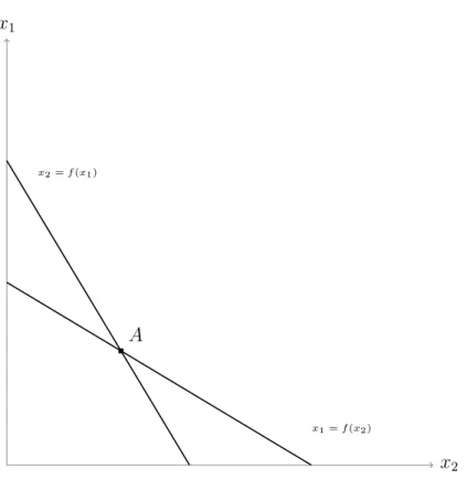
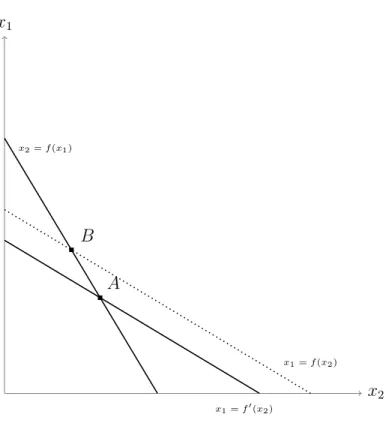
Equations (4) and (5) are the fiscal best responses for countries 1 and 2, respectively. They show, in a (x2,x1) space.

Substituting (5) in (4) yield the Nash Equilibrium values for spending, which are given by:

x1N = − 1 a11[(y ∗ 1− ¯y1) − c(π0− πe) − a21(_a1₂₂(y2∗− ¯y2) − c(π0− πe) − 2_θ2β_a22 22)] − 2 β1 θ1a211 a21a12 a11a22 − 1 (5) x2N = − 1 a22[(y ∗ 2− ¯y2) − c(π0− πe) − a12(_a1₁₁(y1∗− ¯y1) − c(π0− πe) − 2_θβ1 1a211 )] − 2 β2 θ2a222 a12a21 a22a11 − 1 (6)

x1

x2

x2= f (x1)

x1= f (x2)

A

Figure 1: Best Response functions

Point A in figure 1 shows the Nash equilibrium values for spending (x2N, x1N). The functions

are the result of a small calibration of the model, assuming: aii> 1, aij < 1, θi > 0.

4.1

Equilibrium Analysis

The results provide 2 best response functions, where each country decides on the appropriate stance on fiscal policy considering the spillover effects from the integrated union partner. Our analysis will focus on country 1, given that country 2 reacts symmetrically.

As expected, an increase in spending from country 2 has a negative effect country 1’s de-cision to spend (∂x1

∂x2)

2_{. As long as both countries are integrated (a}

21 6= 0), an increase in x2 will

lead to a decrease in x1 (and vice-versa). Since spending has a cost (measured by the coefficient

2_{The analysis made in sections 4.1, 5.1 and Conclusion are under the ceteris paribus proviso, if nothing else is said.}

βi, intended to represent the distortionary effects of taxation and its subsequent welfare

decreas-ing effect), countries prefer to absorb the positive externality associated with the spillover-effect (measured by the terms aij) rather than engage in their own fiscal policies.

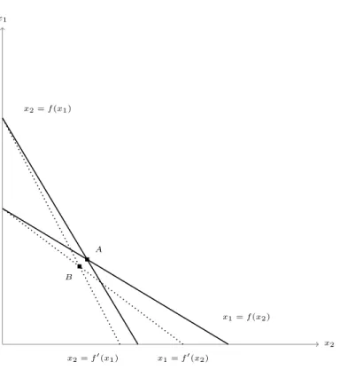
Similarly, an increase in integration has a negative effect on own-country spending (∂x1

∂a21 < 0)

as reflected in Figure 4 (see annex). Increased integration means bigger spillovers, which reduce the need for fiscal expansion. The bigger the increase in integration, the larger will be the decrease in spending. A simultaneous increase in the coefficients of integration (a12 and a21) will have

beneficial effects for both countries only if they are of a similar magnitude. (Fig. 5, see annex). By increasing mutual spillover effects, the need for debt fuelled expansions is reduced.

Naturally, own-country spending decreases with an increase in the cost of debt (∂x1

∂β1 < 0) and

increases with an increase in the natural output gap ( ∂x1

∂(y∗

1− ¯y1) > 0).

Figure 6 shows the effect on x1and x2 of an increase in country 1’s output gap. As expected,

spending in country 1 will increase and spending in country 2 will decrease less-than proportionally (due to the spillover effect).

A change in the fiscal multiplier also affects spending in the following way (∂x1

∂a11 >< 0)

which is generally positive. When (y1 − ¯y1 − x2a21) is negative (or 0), an increase in the fiscal

multiplier will enhance the efficiency of spending, consequently leading to a larger gap (which we model to be welfare reducing). For this reason, when the gap is negative or 0, an increase in a11will

induce a decrease in spending. Similarly, a sufficiently high cost of debt (4β1 > (y1− ¯y1− x2a21))

can have an identical effect.

Finally, the degree of inflation aversion (θi) also affects the equilibrium solution. A decrease

(∂x1

∂θ1 > 0). Figure 7 represents the change in equilibrium with an increase in θ1

Since output in both countries is affected by the inflation differential, so are the fiscal policy stances. As such, the best response of both countries to an increase in surprise inflation will gen-erally be a decrease in expenditure ( ∂x1

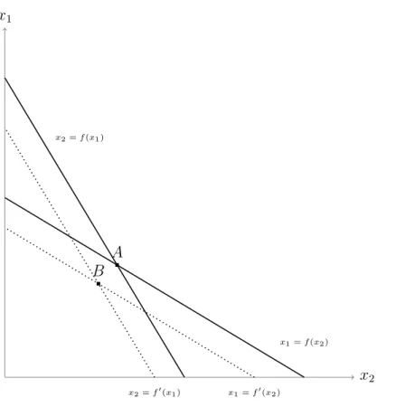
∂(π0−πe) > 0). Figure 6 represents the effect of an increase in

surprise inflation. The CB can, therefore, induce growth in both economies by choosing a rate such that π0 > πe. x1 x2 x2= f (x1) x2= f0(x1) x1= f0(x2) x1= f (x2) B A

Figure 2: Effect in x1and x2of an increase in surprise inflation (π0− πe). Equilibrium moves from

point A to point B.

Equations (6) and (7) show the Nash equilibrium values for spending. It may be interesting to explore the effect of changes in inflation aversion in the equilibrium solution: ∂x_∂θ1N

2 < 0. The

result is generally negative since a11, a22 > 1 and a12, a21 < 1, which means that an increase in

that a small θ2can generate consecutively high values for x1.

Considering the framework of our model, fiscal decisions in a large economy - which we will define as one with high crossed-spillovers ( aij) - are extremely important, since they have

a strong effect on its integrated partners. If such a country (let’s say country 1) has persistently high inflation aversion (small θi), spending will be severely curbed, generating fewer spillovers

to its integrated partner, and ultimately decreasing its output. To maintain the desired output gap, country 2 will be forced to use its own fiscal policy to expand GDP - an unwanted solution, since debt is welfare reducing. This scenario can aggravate if the cost of debt in such countries is too high, generating further welfare losses. One can easily expand this result to an N country framework, where a large economy is one that strongly affects several integrated partners through crossed spillovers ( a1n).

Another interesting conclusion is the effect in x1of changes in country 2’s output gap ( ∂x_1N ∂(y∗₂− ¯y2)),

which is negative since a11, a22 > 1 while a12, a21 < 1. An increase in country 2’s output gap will

induce a decrease in expenditure in country 1 - since country 2 will have to increase spending to bring GDP up to the desired level, country 1 can ”freely” appropriate the positive spillovers, thereby avoiding the cost of debt-fuelled expansions. Since we postulated for the existence of y_i∗as a level of GDP that is cleared of monopolistic competition (see section 3), this measure of output gap (y_i∗ − ¯yi) can be seen as a measure of the natural efficiency of the economy. Countries with

naturally efficient economies - yielding a consistently low output gap - will generally require a smaller amount of fiscal stimulus. This will leave its integrated partners in a weaker position: a less efficient economy - one that requires a larger amount of government spending - will be left to its own means since it cannot overly depend on the few externalities from its more efficient partner.

5

Fiscal Leadership

With Fiscal leadership we want to study how policy interactions change if x1 and x2 are

exoge-nously defined.

t=0 t=1 t=2

In t=0, expectations on inflation are formed (πe_{). In t=1, both countries exogenously decide on}

spending (x10 and x20), given expectations (π

e_{) but independently of each other. In t=2, the CB}

chooses its desired inflation rate based on expectations (πe) and given both values for spending (x10 and x20).

The CB’s loss function is minimized given the chosen fiscal stances: (x10, x20)

min π Lm = 1 2θm 2 X i=1 λi(yi∗− yi)2+ 1 2π 2 s.t ( x1 = x10 x2 = x20 FOC: π + θmλ1(y1∗− y1)(−c) + θmλ2(y∗2 − y2)(−c) = 0 π = θm[λ1(y∗1 − y1)(c) + λ2(y∗2− y2)(c)]

Which can be rearranged to: π = θmc[λ1(y ∗ 1 − ¯y1− a21x20 − a11x10 + cπ e_{) + λ} 2(y2∗− ¯y2− a12x10 − a22x20 + cπ e_)] 1 + θmc2 (7)

5.1

Equilibrium Analysis

Equation (8) describes inflation setting by the common central bank in a context where it has discretion over monetary policy. In this case, the CB accommodates the output gap should fiscal policy (by itself) be unable to bring yito the desired level. Surprise inflation can be created to affect

output and bring it to the desired level.

If both economies are already at such levels through own-country fiscal policies and spillovers, then inflation will be set at:

π = θmc(λ1.cπe+(1−λ1).cπ)

1+θmc2

The optimum inflation rate is also negatively affected by spending in each country (_∂x∂π

i0 < 0).

A larger level of spending will affect output in both countries, either directly or indirectly through the fiscal spillovers.

Considering both economies with a positive output gap, the Central Bank will always set a positive value for inflation such that agents are surprised π > πe _{- thereby increasing output. An}

increase in inflation expectations (πe) will generate higher actual inflation - the opportunity cost (smaller GDP) of desinflating the economy is higher than the loss in increased inflation (_∂π∂πe > 0).

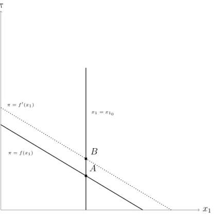
Inflationary policy by the CB is chosen by considering political weights at the country-level: λi. A country which is more heavily weighed by the CB (large λi) moving away from its desired

output level requires stronger action and, as such, cause a more hawkish response (_∂λ∂π

1 > 0).

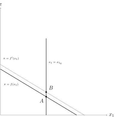
Figure 3 shows the above mentioned effect, considering a small calibration of the model with π > 0, y1 < y1∗; y2 < y2∗:

π x1 π = f (x1) π = f0(x1) x1= x10 A B

Figure 3: Effect in π of an increase in λ1(for a fixed x2, given x1 = x10)

As expected, for a given level of spending (x1 = x10) such that there is a positive output gap,

a larger λ1 will lead to an increase in inflation.

In the case where one of the countries (but not both) is already at the desired output ( ¯y1 +

a21x2+ x1a11= y∗1, y2 < y2∗), we will have:

π = θmc[λ1(−cπe)+λ2(y∗2− ¯y2−a12x₁₀−a22x₂₀−cπe)]

1+θmc2 .

In such a situation, the degree of accommodation of the CB will depend on the relative weight of each country. If λ2 is small enough, it is optimum for the CB to avoid committing to any

expansionary policy. The absence of surprise inflation will benefit the larger economy - country 1 - at the expense of a welfare-decreasing output gap in the smaller one. Use of fiscal policy will be the only possible driver to achieve y₂∗, but if the cost of debt is too big a burden for country 2, or if there is any debt ceiling, then the necessary push toward the optimum output level will not occur,

leaving the economy further from the bliss point.

Finally, an decrease in the CB’s inflation aversion, given by an increase in θm, will have a

positive impact in the chosen inflation rate _∂θ∂π

m > 0. This solution will tend to enhance the CB’s

extent of intervention in the economy, which should benefit the smaller countries, which, in this framework, tend to be more neglected. Figure 8 (see annex) graphically depicts this effect.

6

Discussion and application to EMU

We divide the Euro experience in two moments, both of which are well captured by our model. The Monetary Leadership equilibrium illustrate some features of the early Euro years: the European Central Bank is generally more conservative than the fiscal authorities, and commits to a given inflation rate based on which policy-makers chose an appropriate (and feasible) level for spending. Inversely, the sovereign debt crisis years (and, arguably, up to the present day) have witnessed a greater effort by the ECB to accommodate shocks, especially in its attempt to ease borrowing conditions for peripheral countries through non-conventional policies. Such behaviour is equally well captured by our Fiscal Leadership equilibrium.

In the build-up to the sovereign debt crisis of 2011, peripheral EMU countries like Ireland, Cyprus, Greece and - to some extent - Portugal (alongside some others), fuelled their growth on increased spending Overbeek (2012) made accessible by cheap credit that ”flooded South after the creation of the Euro” (Krugman (2012)). By 2011, the German general government deficit (as % of GDP) had decreased 44% since 2000. Inversely, Portugal or Greece had seen their deficits inflated by 138% and 153%, respectively. Naturally, cost of debt soared, forcing both Portugal and Greece to ask for bailout programs in mid 2011 (as well as Cyprus, Ireland and Spain). By

2012, the yield on Portuguese and Greek Long-term treasury bonds was up to 12,8% and 29% respectively. Although we do not specifically model for continuous time, our model shows how specific conditions, like large output gap differentials or significantly different degrees of inflation aversion can contribute to permanent overspending. Given a framework of commitment by the CB (see section 4, Monetary Leadership), debt accumulation (and the consequential rise in its cost) is the likely result of these unbalanced equilibria.

Moreover, a study by Scheve (2004) showed that, controlling for economic performance, preferences regarding inflation vary substantially across EMU members: German citizens have a general inflation aversion of 0,296, compared to -0,757 for Portugal and -0,252 for Greece3. These results support the aforementioned conclusion that high inflation aversion in a large country will lead to significant imbalances within a MU. This contrast not only explains how inflation can affect GDP through decreased spending (smaller spillovers), it also sheds some light on why the ECB’s response to the crisis was so sluggish. In a context were the CB is a second mover (see Fiscal Leadership, section 5), we proved that the monetary authority may not want to increase inflation if the output gap affects a small economy (small λi). In this context, it may be optimal for a

conservative CB to remain doveish, keeping inflation at bay while accepting the output gap. Only when the crisis started to hit larger countries like Spain and Italy - yields on spanish and italian debt started rising in late 2011/mid 2012, with rates at a maximum of 6,8% and 7%, respectively - did the Central Bank start to act aggressively, i.e. with the ”Whatever it takes” speech by ECB president Mario Draghi, in August 2012.

Finally, data from the OECD reveals that in the last 19 years, the average output gap in

3_{values are relative to inflation aversion in the UK, which explains the negative numbers although they do not}

Germany has been -0,228, comparing with -1,467 for Portugal and -3,325 for Greece (as % of GDP). These results suggest that the German economy has a smaller ”natural” output gap vis-`a-vis its southern European partners. Lower spending in Germany may not only be explained by high inflation aversion but, critically, by a smaller need to spend. In the long run, permanently different output-gaps will generate a natural unbalance: underspending in one country will have to be compensated with overspending in the others, with the effect being broader if the country at stake is large enough. Any serious attempt at economic convergence on the union level will be thwarted if such structural differences prove to be enduring. The problem is exacerbated due to several fiscal constraints imposed by the SGP, particularly in the form of debt ceilings (Soukiazis and Castro (2005)).

7

Conclusions

We develop a 2-country model of asymmetry and heterogeneity to study interactions in mone-tary and fiscal policies in the context of a Monemone-tary Union. A common Central Bank decides on monetary policy through an effective rate of inflation, and fiscal policymakers chose their desired spending. Output in both countries is affected by spillovers from their partners’ fiscal policy de-cisions - positively in case of an expansionary fiscal policy; negatively otherwise. The 3 players act according to a Social Loss function, positive in the output gap and in inflation. We model debt to be welfare decreasing by adding it to the Social Loss functions in both countries, weighed by a coefficient to represent its cost.

We find that, considering a Monetary Leadership framework - when the CB commits to a given inflation target and both countries respond with fiscal policies - the existence of surprise

inflation (π − πe) and of a large output gap (y∗_i − ¯yi) will increase spending in equilibrium. Our

results also show that received spillovers (aji, considering an analysis of country i) account for a

decrease in spending. On the other hand, an increase in the cost of debt or in inflation aversion (θi)

will typically increase spending. Increases in the fiscal multiplier (aii) will have the opposite effect.

We highlighted how the behaviour of an integrated partner can affect a country’s fiscal policy decisions. An increase in inflation aversion in a partner country (smaller θj) as well as a decrease in

its output gap (y_j∗− ¯yj) will induce a spending increase in country i. We suggest that these factors

can contribute to explain the debt dynamics in Europe over the last 20 years, particularly explaining why peripheral European nations overspent while Germany accumulated successive fiscal superav-its. Introducing subsequent periods could be an important extension to the model, as it would shed light on the debt-dynamic effects of our findings: continuous overspending puts pressure on bond prices, which increases the cost of debt (βi), with an effect on the equilibrium values for spending.

In the Fiscal Leadership specification, the CB chooses its optimum inflation rate given the exogenously chosen fiscal policies of each country. Results show that the inflation rate chosen by the CB is positively influenced by a decrease in inflation aversion - θm - and by a decrease in

the coefficients for integration (aji and aij). Considering the existence of a positive output gap

(y∗_i − yi > 0), an increase in the coefficients of integration (aij and aji) will decrease the optimum

inflation rate, given that the increased spillovers will contribute to an increase in GDP. Similarly, an increase in spending in each country (xiand xj) will serve to decrease the chosen inflation rate,

since it positively affects output (either directly or indirectly, through spillovers).

Finally, the optimum rate of inflation also changes according to the coefficient of country weights, λi. A very small λi will generate doveish responses by the CB, leading to very weak

ac-commodative policies. This bias against smaller economies is a significant design flaw in the EMU, given that the European Central Bank is, frequently, the only institution with effective ability to ex-ecute macroeconomic policy (most of the smaller nations are constrained on the fiscal instrument by strict debt ceilings or high cost of debt).

Our model suggests that any growth in integration - modelled as increases in aij and aji

-will be mutually beneficial only if both move simultaneously and have similar magnitudes. In the Monetary Leadership framework, a simultaneous increase in both measures of integration will lead to a decrease in expenditure for both countries. In the Fiscal Leadership framework, increasing spillovers will positively affect output in both countries, inducing the CB to chose a lower rate of inflation.

To conclude, EMU faces several challenges for the next decade. Further economic integra-tion, particularly at the fiscal level, should be sought only if it is implemented in a coordinated man-ner. Heterogeneity at the social level - like country-specific degrees of inflation aversion - should be acknowledged and, over time, ought to be harmonized. Finally, the European Central Bank’s policy-setting should be reviewed in order to mitigate the misrepresentation of smaller economies.

References

Afxentiou, P.C., 2000. Convergence, the maastricht criteria, and their benefits. Brown J. World Aff. 7, 245.

Alesina, A., Tabellini, G., 1987. Rules and discretion with noncoordinated monetary and fiscal policies. Economic Inquiry 25, 619–630.

Barro, R.J., Gordon, D.B., 1983. Rules, discretion and reputation in a model of monetary policy. Journal of monetary economics 12, 101–121.

Bayoumi, T., Eichengreen, B., 1992. Shocking aspects of european monetary unification .

Beetsma, R.M., Bovenberg, A.L., 1999. Does monetary unification lead to excessive debt accumu-lation? Journal of Public Economics 74, 299–325.

Bergsten, C.F., 2012. Why the euro will survive: Completing the continent’s half-built house. Foreign Affairs , 16–22.

Buiter, W., Corsetti, G., Roubini, N., 1993. Excessive deficits: sense and nonsense in the treaty of maastricht. Economic Policy 8, 57–100.

Chari, V.V., Kehoe, P.J., 2007. On the need for fiscal constraints in a monetary union. Journal of Monetary Economics 54, 2399–2408.

Corsetti, G., Meier, A., M¨uller, G.J., 2009. Cross-border spillovers from fiscal stimulus .

De Grauwe, P., 1996. The economics of convergence: Towards monetary union in europe. Weltwirtschaftliches Archiv 132, 1–27.

Dixit, A., Lambertini, L., 2003a. Interactions of commitment and discretion in monetary and fiscal policies. American economic review 93, 1522–1542.

Dixit, A., Lambertini, L., 2003b. Symbiosis of monetary and fiscal policies in a monetary union. Journal of International Economics 60, 235–247.

Frankel, J.A., Rose, A.K., 1998. The endogenity of the optimum currency area criteria. The Economic Journal 108, 1009–1025.

Kalemli-Ozcan, S., Sørensen, B.E., Yosha, O., 2001. Economic integration, industrial specializa-tion, and the asymmetry of macroeconomic fluctuations. Journal of International Economics 55, 107–137.

Kennen, P., Mundell, R., Swoboda, A., 1969. The theory of optimum currency areas: An eclectic view.–monetary problems of the international economy.

Krugman, P., 1993. The transition to economic and monetary union in europe, chapter lessons of massachusetts for emu.

Krugman, P., 2012. Europe’s Austerity Madness. URL:

https://www.nytimes.com/2012/09/28/opinion/krugman-europes-austerity-madness.html. Kydland, F.E., Prescott, E.C., 1977. Rules rather than discretion: The inconsistency of optimal

plans. Journal of political economy 85, 473–491.

Luque, J., Morelli, M., Tavares, J., 2014. A volatility-based theory of fiscal union desirability. Journal of Public Economics 112, 1–11.

McKinnon, R.I., 1963. Optimum currency areas. The American economic review 53, 717–725. Mundell, R.A., 1961. A theory of optimum currency areas. The American economic review 51,

657–665.

Overbeek, H., 2012. Sovereign debt crisis in euroland: root causes and implications for european integration. The International Spectator 47, 30–48.

Pereira, M., Tavares, J., 2019. Extracting implicit country weights in ecb’s monetary policy . Rogoff, K., 1985. The optimal degree of commitment to an intermediate monetary target. The

quarterly journal of economics 100, 1169–1189.

Romer, D., 2006. Advanced macroeconomics 3rd edition mcgraw–hill .

Scheve, K., 2004. Public inflation aversion and the political economy of macroeconomic policy-making. International Organization 58, 1–34.

Soares, M.J., et al., 2011. Business cycle synchronization and the euro: A wavelet analysis. Journal of Macroeconomics 33, 477–489.

Soukiazis, E., Castro, V., 2005. How the maastricht criteria and the stability and growth pact affected real convergence in the european union: A panel data analysis. Journal of Policy Modeling 27, 385–399.

Svensson, L.E., 1997. Inflation forecast targeting: Implementing and monitoring inflation targets. European economic review 41, 1111–1146.

Annex

Figure 4: Effect in x1 and x2 of an increase in a21

x1 x2 x2= f (x1) x1= f (x2) x1= f0(x2) x2= f0(x1) A B

x1 x2 x2= f (x1) x1= f (x2) x1= f0(x2) A B

Figure 6: Effect in x1and x2of an increase in y1∗− ¯y1

x1 x2 x2= f (x1) x1= f (x2) x1= f0(x2) A B

π x1 π = f (x1) π = f0(x1) x1= x₁₀ A B

Figure 8: Effect in π of an increase θm (for a fixed x2, given x1 = x10)

1.

= −

2.

= −

3.

=

4.

=

5.

= −

− 4

6.

= −

7.

=

8.

= −

9.

=

10.

=

= θ

c

_{+ 1}

11.

=

12.

=

θmc[(y₁∗− ¯y1−a21x2−a1x1−cπe)]

1+θmc2

13.

m

=

c[λ1(y₁∗− ¯y1−x2a21−x1a11+cπe)+λ2(y∗₂− ¯y2−x1a12−x2a22+cπe)]